An adaptive spectral index for carbonate rocks using OLI Landsat-8 imagery

Abstract

The accurate characterization of carbonate rocks is crucial for determining the potential for exploring outcrops in the oil industry. Modern remote sensing instruments have played an important role in estimating mineral characteristics in the most varied scales. However, mathematical expressions suggested for converting radiance values to mineral information are often designed to work in only one particular territory. At the same time, the few general solutions existing tend to achieve overall poor results. In this paper, we propose an adaptive approach to estimate subpixel amounts of carbonate rocks using OLI-Landsat 8 image data. The main formulation is derived from exhaustive analysis of the spectral behavior of several carbonate materials. The formulation is subsequently adapted through the use of a genetic algorithm to work on diverse situations. Experiments have demonstrated the adaptability of the method for different environments, as well as its higher performance when compared with existing carbonate indices.

Keywords:

• Carbonate rocks
• spectral index
• adaptive system
• outcrops
• unmixing model

1. Introduction

Carbonate rocks contain most of the world’s hydrocarbons like oil and gas, serving as hosts for important mineral deposits. An efficient way to investigate carbonate reservoirs at great depths is the analysis of analogous outcrops (Basso et al. 2017), since they can provide information about essential parameters that would be impossible to achieve directly (e.g. mineral composition, geophysical, and geochemical properties) (Marques et al. 2020). Despite its recognized value for the oil industry, field campaigns in outcrops present several drawbacks (Xie et al. 2015). They are time-demanding because outcrops extend through a vast territory, and are labor-intensive since they are located in inhospitable places and usually present many obstacles to reach. The mentioned limitations make remote sensing images a convenient alternative to study carbonate outcrops (Asadzadeh and de Souza Filho 2020).

Carbonates have important spectral features located at Short Wave InfraRed (SWIR) and Thermal InfraRed (TIR) spectral regions (Rencz and Ryerson 1999; Malainine et al. 2022). Analyzing the detailed spectral response in the entire spectrum is crucial to differentiate them from other minerals (e.g. silicates, oxides, sulfides) or remaining targets present in outcrops (Crowley 1984; de Linaje et al. 2018). However, sensor technology could not yet retrieve orbital hyperspectral images with pixel size and spectral resolution equally adequate for such complex applications (Yue et al. 2010). Furthermore, most of the existing remote sensing approaches designed for popular sensors rely on simple formulations that usually underestimate the spectral information capabilities or present a level of generalization that dramatically impact the accuracy of the analysis (Xie et al. 2015; Xue and Su 2017).

The most promising approaches apply spectral indices - dimensionless variables derived from pre-calibrated equations - developed to indicate the presence of particular materials inside pixels (Yue et al. 2010; Pei et al. 2018; Adelabu et al. 2020; Alexander 2020; Huynh et al. 2021). Spectral indices have applications in several remote sensing fields, such as vegetation, hydrology, urban, and geological studies (Cao et al. 2017; Bouhennache et al.; Qu et al. 2021). Although, for carbonate rocks, few indices are available, restricted to the most popular instruments (e.g. OLI-Landsat 8 and MSI-Sentinel), and are often strictly designed for a specific region (Tangestani and Shayeganpour 2020; Baranwal et al. 2022). In Pei et al. (2018), OLI-Landsat 8 imagery was used to estimate exposed bedrock fractions in karst regions (environments developed in dense carbonate rocks). The methodology was designed for typical regions of southwest China to distinguish exposed bedrock from other typical classes. In Xie et al. (2015), two carbonate indices were proposed through a model representing the relationships between the index and the fractional covering of carbonates in karst rocky desertification. The application is particularly interesting since the index proposed was designed to provide the actual content of materials in multispectral images. Experiments performed in a specific area proved the superiority of the index when compared with other formulations and the linear unmixing model. Spectral measurements were collected in the field in Yue et al. (2010) to develop carbonate rock fractions in exposed bedrock. Compared with linear spectral unmixing, the work showed that carbonate rocky desertification could be extracted relatively simply with the combination of vegetation indices.

Although many applications use spectral indices to monitor mineral conditions in varied scales, spectral mixture models are also employed in similar applications and are able to reach interesting results (Saha 2022). In this case, the proportions of land cover at the sub-pixel scale can be theoretically estimated. However, the use of this approach is limited by the variability of endmembers (components in the mixture), especially for highly heterogeneous landscapes in carbonate regions Genú et al. (2013). Furthermore, defining endmembers spectra of such complex targets is an error-prone task Zanotta et al. (2014).

As expected, works that used spectral indices for estimating parameters in carbonate environments for specific locations tend to present inappropriate results in different sites (Muller et al. 2020; Piyoosh and Ghosh 2022). It happens because the calibration of equations is made to supply specific requirements of determined applications. In this paper, we propose an adaptive spectral index to compute carbonate concentrations in outcrops using the multispectral OLI-Landsat 8 data. The formulation is based on previous studies that indicate optimal practices for designing spectral indices for remote sensing sensors, as well as further adaptation strategies. In the first step, a collection of samples is used to determine the best features and analytical terms for establishing the relationship between OLI-Landsat 8 spectral channels and the corresponding amount of carbonates (source domain). In the second step, adaptation is made by adjusting the original formulation to accommodate different situations (target domains) through a supervised genetic algorithm.

2. Background and problem formulation

2.1. From radiometric measurements to the spectral index

Most of the methods to analyze radiative measurements are based on a correct understanding of the physical processes that resulted from the observations. Essentially, the models involve a large set of radiative variables describing the source and the interaction of the radiation with all elements on the ground (Govaerts et al. 1999; Yang et al. 2017). Analytically, a single remote sensing measurement R may be described by a model of the type (1) $$R=r(\mathbf{X},\mathbf{Y}),$$(1) where vector $\mathbf{X}=x_1,x_2,\dots ,x_n$ carries the instrument parameters of the measurement, like sensor and optics characteristics, which are independent variables known at the time of image acquisition, and $\mathbf{Y}=y_1,y_2,\dots ,y_n$ includes physical parameters like atmospheric and target properties (Verstraete and Pinty 1996). Usually, the values for the independent variables in X are fully known. However, there is a redundancy in the values of Y, since more than one combination of them can result in the same measurement R, which makes the general problem ill-posed. Nonetheless, some conditions can be assumed to reduce the number of dependent variables in Y, and shall be discussed in what follows.

Initially, the aim is to identify in the raw data the processes that are not directly related to the phenomenon of interest, such as those instrument effects that can be modeled included in X and assumed to be separated from the remaining and yet unknown processes. This task involves isolating and removing errors resulting from inaccurate corrections and noise in the data. Since the objective separation between each independent variable is a difficult task, the application of this approach often makes use of data collected in parallel with the measurements (Zheng et al. 2018). Traditionally, a solution for this approach is the inverse problem of estimating the most likely values of multiple variables of Y using mathematical models that describe how the dependent variables affect the measurements in R (Yang et al. 2017). Recently, modern approaches make use of computational intelligence, like supervised machine learning, which is able to model the general behavior of a complex phenomenon from the collection of training samples, since they are usually insensitive to small uncertainties and imprecise sampling (Bouhennache et al. 2019).

Assuming that sufficient ground samples and reliable ground truth are available, the relationship between observed reflectance measurements and the elements of interest for the index can be adequately established by powerful regression algorithms (Cao et al. 2017). With main features identified, spectral indices can be made sensitive or insensitive to various processes by manipulating the mathematical definition involving variables representing the features. Graphically, this corresponds to positioning, orienting, and bending a multidimensional surface to fit a condition that empirically satisfies the user expectations, achieving the desired degree of sensitivity for each case (Fulcher 2008). In the next section, we define the source domain and target domains, including three different outcrops and the features of interest to be included in the index formulation and its further adaptation.

2.2. Geological settings and study areas

The three outcrops used in this study are located in Brazilian Northeast, more precisely in the Jandaíra Formation, belonging to the onshore portion of the Potiguar Basin (Figure 1A) (Soares et al. 2003; Pessoa Neto et al. 2007). This basin originated in the Jurassic-Cretaceous period and is composed of rift, transitional, and post-rift sedimentary units (de Oliveira et al. 2013). The Jandaíra Formation is part of the post-rift sequence in the Turonian-Campanian (93.9 − 83.6 Ma) (Oliveira et al. 2013) and appears as a carbonate ramp 150 km wide and 250 km long, ranging from 50 to 700 m in thickness with the Açu Formation at its base (Silva et al. 2017). The Jandaíra Formation is made up of bioclastic (green and red algae, milliolides, mollusks) and oolitic calcarenites, calcilutites with planktonic and benthic foraminifera and calcilutites with bird’s eyes (Silva et al. 2017). In addition, grains of primary carbonates (calcite) are transformed into dolomite, giving rise to karstification events (Menezes et al. 2020).

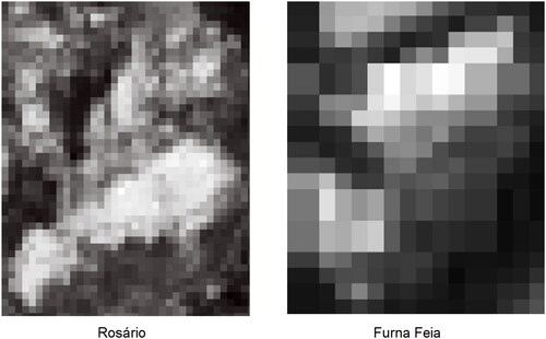
Figure 1. Geological map of the Potiguar basin (A), and the three outcrops placed in the Jandaíra formation: Soledade (B); Rosario (C); and Furna Feia (D).

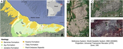
The Soledade outcrop (Figure 1B), was initially chosen to provide the necessary data for carbonate index formulation (i.e. the source domain). Soledade outcrop is composed of carbonates (mainly calcite and dolomite) surrounded by small trees, shrubs, and bare soil characteristics of the area. The rocks of Soledade are mostly composed of mudstones and grainstones, deposited in a marine platform environment as a carbonate ramp, and post-diagenetic carbonate tuffs, presenting intense fracturing, dissolution, and karstification. Two more outcrops (Furna Feia and Rosário) are present in the surrounding region displaying distinct geologic characteristics, types of soil, and vegetation arrangement (Figures 1C and D). They shall be used in this work to promote and assess the adaptation procedures proposed (i.e. the target domains). Despite being spatially close, Soledade outcrop (B) has diverse structural and composition characteristics compared with Rosário (C) and Furna Feia (D) outcrops. Soledade has carbonates more isolated in a preferable area, whereas Rosário and Furna Feia have carbonates mixed with shrubs and small trees. Also, vegetation near Furna Feia is composed of different species, which can be noticed by the color surrounding the mineral deposits at the center of the scene. These aspects are highly desirable since the proposed approach assumes that the initial formulation is unable to achieve acceptable results for multiple situations, but after adaptation, it becomes effective again to fit other specific carbonate presentations.

2.3. Data mining and feature selection

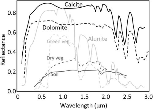
Previous understanding of processes that link the spectral reflectance of the materials to the desired information is critical for designing the spectral index optimized for a particular application. Thus, according to Bouhennache et al. (2019), the regions with the same value of the index on the multispectral space (isolines) can be adequately located and a multidimensional region can be generated representing the relationship between observed spectral amounts and expected index values. As can be seen in Figure 2, carbonate minerals have important reflectance features in visible (0.4 − 0.7 $\mu m$) and SWIR (0.9 − 2.5 $\mu m$) regions of the electromagnetic spectrum, mainly for Calcite and Dolomite, the most common carbonates on the Earth (Zaini et al. 2012). Conversely, other materials usually present in carbonate outcrops like green vegetation, dry vegetation, soil, and alunite (Ford and Williams 2013), show lower values in these regions. Thermal infrared features can also be considered for the identification of carbonate materials. However, thermal channels are rarely present for the majority of multispectral scanners or, if any, the pixel size is very large (in the order of hundreds of meters), not suitable for most applications.

Figure 2. Reflectance spectra for visible and NIR regions of calcite (solid black), dolomite (dashed black), and typical natural targets: dry vegetation (dashed gray), soil (solid gray), Alunite (solid light gray), green vegetation (dashed light gray). Data from Rencz and Ryerson (1999).

To differentiate carbonate rocks from other targets in the studied outcrops, we performed data mining experiments by using simulated and real OLI-Landsat 8 data. OLI-Landsat 8 data has nine spectral bands ranging from VIS to SWIR with spatial resolutions ranging from 15 m (panchromatic) to 30 m (multispectral). The temporal resolution is 16 days.

2.3.1. Regression with simulated data

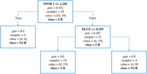
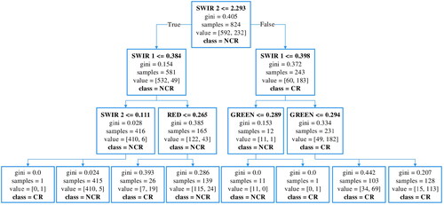
We selected spectral signature readings from a Spectral Evolution SR-3500 spectroradiometer to simulate OLI-Landsat 8 channels over a collection of 19 carbonate rock samples acquired in different positions of Soledade outcrop. Spectral Evolution SR-3500 spectroradiometer covers the visible and infrared spectra using three photodiode arrays with no moving parts. It can collect 2151 channels from VIS to NIR in as little as 100 milliseconds. The measured spectra were used along with the response curve of the sensor to simulate an output of each pixel purely occupied by the sample. The same process was made for the non-carbonate elements also present near the outcrop. Examples of many kinds of bare soil, vegetation, water, and other minerals (silicates, oxides, sulfides, etc.) were used to simulate the outcrop surroundings, by means of spectral signatures imported from the public United States Geological Survey (USGS) spectral library. The rationale behind this experiment was to guarantee the representation of pure materials, which is not easily reachable when dealing with real pixels. Spectral responses of the relevant materials were inserted in a Classification and Regression Tree (CART) algorithm (Steinberg 2009) to highlight features with decisive discrimination power between carbonate (CR) and remaining non-carbonate (NCR) targets (Arvor et al. 2013). Figure 3 shows that SWIR 2 channel (2.11-2.29 $\mu$ m) is at the top of the hierarchical sequence, followed by the color blue channel (0.45-0.51 $\mu$ m). The Gini importance index was reported to demonstrate the relevance of each node of the hierarchical tree.

Figure 3. Decision tree for simulated OLI-Landsat 8 data using carbonate rocks against several materials including types of vegetation, different kinds of rocks, bare soils, and water in varied conditions. The carbonate samples were grouped standing by CR class, whereas the remaining non-carbonate classes were all merged to represent NCR class. The result indicates SWIR 2 as best discriminating parameter, followed by visible channel blue.

2.3.2. Regression with real OLI-Landsat 8

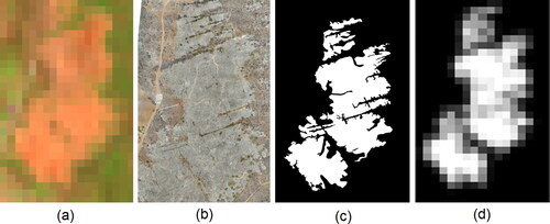
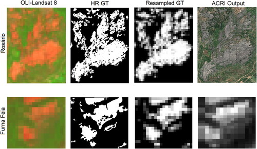
We also selected a set of real OLI-Landsat 8 multispectral pixels (Figure 4a) acquired in September 2020 with corresponding ground truth near the same region where the rock samples were collected, as well as pixels including other materials than carbonates. In this second experiment, the proportions of materials inside each pixel were determined using ground truth obtained from Unmanned Aerial Vehicles (UAV) orthomosaic few days before the satellite acquisition (Figure 4b). The high-resolution color image with a spatial resolution of 0.05 m was visually interpreted by a geologist with expertise in carbonate outcrops to recognize the ground classes. The visual delimitation resulted in a high-resolution binary mask identifying precisely the limits of carbonate rocks in the outcrop area, as depicted in Figure 4c. Finally, the binary map was resampled to achieve the actual size of OLI-Landsat 8 pixels (Figure 4d) with proportions of carbonate rock inside each pixel represented in gray levels. CR class was defined for all pixels presenting more than 50% of carbonate covering, and NCR otherwise. This experiment was particularly useful to highlight the discrimination power of spectral channels in pixels containing carbonates in mixtures with other elements.

Figure 4. (a) OLI-Landsat 8 RGB 5 654 color composition (b) UAV orthophoto of the outcrop area (light gray region) mainly composed of calcite with some areas of dolomite. (c) The ground truth (GT) is generated from the visual interpretation assisted by an expert in the field. (d) Is the corresponding GT of (c) resized to match the Landsat 8 pixel.

As shown in Figure 5, SWIR 2 (2.11-2.29 $\mu$ m) and SWIR 1 (1.57-1.65 $\mu$ m) are at the top positions of the CART output. Visible channels are at the bottom positions. The current result is similar to the previous experiment, except for the size of the CART, which is larger due to the higher quantity and diversity of input data, and the specific visible channel with best power of discrimination. As could be initially inferred from Figure 2, the CART experiments confirm that SWIR and visible channels (blue for the simulated data and red/green for real data) are the best-discriminating features along the spectrum.

Figure 5. Decision tree produced for real OLI-Landsat 8 pixels with carbonate rocks against other present materials including many types of vegetation, bare soil, and minerals. In agreement with the previous experiment, it also indicates the SWIR region with the best discriminating parameter, followed by visible channels. Similar to what was made in the simulated experiment, the carbonate samples were grouped standing by CR class, whereas the remaining non-carbonate classes were all merged to represent NCR class.

2.3.3. Spectral analysis

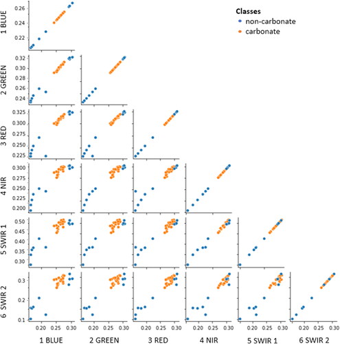
We performed an additional investigation by building scatterplots confronting the OLI features aiming to visualize the boundaries that separate CR and NCR classes spatially. This experiment was useful to highlight where the classes are concentrated in the multispectral space. We produced scatter plots for every two-by-two available channels showing the actual class of the pixels (CR or NCR). As in the previous data mining procedure, scatter plots were built for both simulated and real OLI-Landsat 8 pixels.

Different from the CART experiment, here we formed the NCR class by gradually mixing the spectrum of the materials. The mixing among NCR materials was achieved by adding small increments of each element to simulate all possible combinations inside a pixel. CR was defined by the same gradual mixing among carbonate samples. In such a manner, we could guarantee all possible presentations of NCR and CR in the same plot, allowing the correct visualization of the boundaries to guide the formulation of the proposed index. Figure 6 depicts CR pixels in orange and NCR in blue. The prevalence of SWIR channels (mainly SWIR 2) and visible channels (mainly blue) as best discriminating features is clearly noticed. Also, transitions between NCR and CR can be observed. CR elements occupy a preferable area around reflectance 0.25 in channel blue and reflectance 0.30 in SWIR 2. Likewise, Figure 7 shows the same experiment but performed with the real OLI-Landsat 8. Similar behavior could be noticed. A large area of the plot was occupied by scattering points, highlighting a dense cluster of CR pixels near 0.27 in channel blue and NCR pixels near 0.30 in SWIR 2.

Figure 6. Scatterplot confronting all OLI channels for assigned pixels of CR and NCR. The blue and SWIR2 bands had the most potential for detecting carbonate rocks.

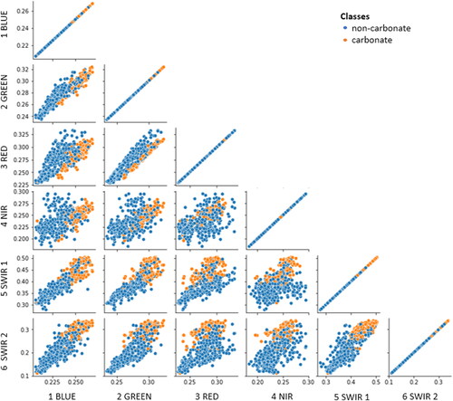
Figure 7. Scatterplot between the classes in the spectral space by comparing two by two the simulated channels of the sensor OLI-Landsat 8. The blue and SWIR2 bands had the most potential for detecting carbonate rocks.

3. Design of optimal carbonate index

3.1. Parameterized index equation

As discussed in (Verstraete et al. 1994), it must be assumed that a change in the variable of interest (e.g. the proportion of CR) will result in a significant variation of a given spectral measurement R. This implies that the system under study in spectral space will be displaced when the property of interest changes. Thus, a type of dependency between the variables will be observed, which can be linear or non-linear.

To design a spectral index sensitive to changes in the amount of CR, it is then sufficient to ensure that the isolines of the index in the multispectral space are able to cross the displacement vector corresponding to these changes. Maximum sensitivity will be achieved when these isolines are perpendicular to such displacements. A logical approach to the design of the spectral index, therefore, consists in first establishing how the radiative property of interest affects the measured spectral reflectances throughout the relevant spectral region, and then deriving the index formula in such a way that its isolines are orthogonal to the displacements.

We can empirically define a surface properly fitting points of interest using the dataset resulting from the scatterplot analysis of Figures 6 and 7. Since the behavior of the data involves a non-linear separation between variables - with a region of high concentration of carbonate elements near the superior vertex of the ellipsis (Figure 6, as well as several non-carbonate elements surpassing the mentioned region according to Figure 7) - we defined a quadratic model of the form (2) $$I=C_1+C_2{\rho }_1+C_3{\rho }_1^2+C_4{\rho }_2+C_5{\rho }_2^2,$$(2) where $C_n$ are the fixed coefficients and ${\rho }_1$ and ${\rho }_2$ the input variables (two selected spectral channels). Equation 2(2) $$I=C_1+C_2{\rho }_1+C_3{\rho }_1^2+C_4{\rho }_2+C_5{\rho }_2^2,$$(2) is a version of the elliptic paraboloid that can be fitted on the data sampled by means of least squares to adjust the $C_n$ coefficients. These coefficients are then achieved by fitting the quadratic curve that best separated the two sampled classes involved according to ${\rho }_1$ and ${\rho }_2.$ For the set of samples used in Soledade, the resulting optimized equation is (3) $$I=\mathit{ACRI}=\frac{1}{65}(25-(\frac{{\rho }_1\cdot 2.45-2.10\cdot {\rho }_2-{74}^2}{600}\left)\right(\frac{{\rho }_2-{28}^2}{23}))$$(3) where ${\rho }_1$ and ${\rho }_2$ now stand for the reflectance of blue and SWIR 2 channels, respectively, and ACRI is our proposed Adaptive Carbonate Rock Index. Figure 8 shows the surface and the corresponding isolines plotted using Equation 3(3) $$I=\mathit{ACRI}=\frac{1}{65}(25-(\frac{{\rho }_1\cdot 2.45-2.10\cdot {\rho }_2-{74}^2}{600}\left)\right(\frac{{\rho }_2-{28}^2}{23}))$$(3) . The resulting plot points out a main region near 30 in the blue channel and 25 in the SWIR 2 channel. The high scores exponentially decrease as the axes values move away from the observed point. Clearly, when the carbonate cover is thin or sparse, the reflectance of both channels is concentrated at low regions (based on sampled Landsat pixels) or around the region of high amounts of carbonate materials. Using Equation 3(3) $$I=\mathit{ACRI}=\frac{1}{65}(25-(\frac{{\rho }_1\cdot 2.45-2.10\cdot {\rho }_2-{74}^2}{600}\left)\right(\frac{{\rho }_2-{28}^2}{23}))$$(3) to compute the index for carbonate rocks of the OLI-Landsat 8 image of Soledade outcrop (Figure 4a) can reach very accurate values when compared with the ground truth prepared using high-resolution image followed by resampling (Figure 9 compared with Figure 4d).

Figure 8. (a) 3-dimensional surface for the original formulation (source domain) of the ACRI index, and (b) corresponding spectral diagram showing isolines designed with reference data from Soledade outcrop. The isolines were important to calibrate zones where the index was more susceptible to the presence of carbonates.

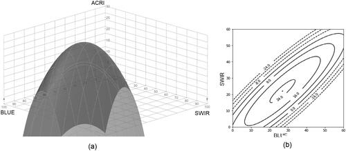
Figure 9. The index result generated using our approach for Soledade outcrop (source domain). Pixels of the index image varies from zero (no carbonates) to one (totally occupied by carbonates).

3.2. Performance evaluation

We selected a set of metrics commonly used to validate the proposed technique against other available approaches, where the ground truth is compared with the predicted values. The first metric was the Mean Absolute Error (MAE), which analyzes the difference between the expected value $y_i$ and predicted value $\widehat{y_i},$ as shown in Equation 4(4) $$\mathit{MAE}(y_i,\widehat{y_i})=\frac{1}{n}\sum _{i=1}^n|y_i-\widehat{y_i}|,$$(4) . (4) $$\mathit{MAE}(y_i,\widehat{y_i})=\frac{1}{n}\sum _{i=1}^n|y_i-\widehat{y_i}|,$$(4)

We also chose the Mean Squared Error (MSE) for an analysis more susceptible to outliers. Since the errors are squared before they are averaged, the MSE provides a relatively high weight to large errors. Then, this metric allows highlighting noticeable discrepancies between the expected value $y_i$ and predicted value $\widehat{y_i}.$ The MSE is given by: (5) $$\mathit{MSE}(y_i,\widehat{y_i})=\frac{1}{n}\sum _{i=1}^n{(y_i-\widehat{y_i})}^2.$$(5)

Although the MAE and MSE metrics are widely used and work well for comparison purposes, they are not sensible to how the models perform absolutely. Thus, we used the coefficient of determination $R^2$ represented by Equation 6(6) $$R^2=1-\frac{\sum _{i=1}^n{(y_i-\widehat{y_i})}^2}{\sum _{i=1}^n{(y_i-\overline{y})}^2},$$(6) for a more specific evaluation. (6) $$R^2=1-\frac{\sum _{i=1}^n{(y_i-\widehat{y_i})}^2}{\sum _{i=1}^n{(y_i-\overline{y})}^2},$$(6) where $\overline{y}$ represents the average of the observed values.

Using the same ground truth for comparison, the proposed equation (ACRI) reached the best scores when compared to existing solutions KBRI (Pei et al. 2018), CRI1 and CRI2 (Xie et al. 2015), NDRI1 (Huang and Cai 2009), NDRI2 (Li and Wu 2015), as well as the popular Linear Unmixing (Shimabukuro and Smith 1991) (Table 1). It is worth noting that the positive result observed was expected since the suggested equation was applied in the same environment where training samples were collected. Figure 9 shows the visual comparison between the High Resolution (HR) ground image and the index generated for the Soledade outcrop. It is also important to notice that, since the equation and its coefficients are calibrated using ground truth based on observed pixels, the resulting index can be seen as a proportion estimator of the area occupied by the specific material in the pixel area.

Table 1. Mean Absolute Error (MAE), Mean Square Error (MSE), and $R^2$ when considering 30 random executions of the 20% image window sampling. Higher mean values indicate better results.

		MAE		MSE		$R^2$
		Mean	Std	Mean	Std	Mean	Std
Furna Feia	ACRI (ours)	0.517	0,41	0.394	0.061	–2.13	0.06
	KBRI	0.834	0.011	0.769	0.014	–0.56	0.26
	CRI1	0.342	0.003	0.129	0.002	–0.05	0.16
	CRI2	0.437	0.016	0.221	0.012	–0.81	0.37
	NDRI1	0.398	0.007	0.177	0.005	–0.44	0.26
	NDRI2	1.048	0.034	1.261	0.061	–1.58	0.52
Rosário	ACRI (ours)	0.607	0.029	0.521	0.045	–2.40	0.11
	KBRI	0.795	0.016	0.718	0.021	–0.17	0.08
	CRI1	0.318	0.006	0.114	0.003	0.24	0.04
	CRI2	0.379	0.009	0.177	0.007	–0.16	0.11
	NDRI1	0.358	0.006	0.148	0.004	0.02	0.08
	NDRI2	0.926	0.022	1.041	0.039	–0.71	0.16
Soledade	ACRI (ours)	0.255	0.038	0.102	0.029	0.18	0.30
	KBRI	0.862	0.013	0.816	0.017	–0.60	0.27
	CRI1	0.383	0.006	0.161	0.004	–027	0.22
	CRI2	0.484	0.021	0.177	0.007	–1.14	0.45
	NDRI1	0.398	0.004	0.148	0.004	–0.37	0.20
	NDRI2	1.013	0.030	1.041	0.039	–1.29	0.44

The best rates are in boldface.

We tested the exact index configuration presented in Equation 3(3) $$I=\mathit{ACRI}=\frac{1}{65}(25-(\frac{{\rho }_1\cdot 2.45-2.10\cdot {\rho }_2-{74}^2}{600}\left)\right(\frac{{\rho }_2-{28}^2}{23}))$$(3) over Rosário and Furna Feia outcrops to assess the performance of the formulation outside the source domain. The outcrops are also composed of carbonate rocks among other materials. The results of Table 1 show us poorer performances when compared to other carbonate indices. In special, CRI1 presented the best performances in both outcrops (boldface values), outperforming our proposed ACRI. These results confirm our initial expectations, indicating that application for other carbonate regions has to be done under calibration of the coefficients to the special characteristics of the target environment. The next section presents the adaptation suggested and the experiments to attest the effectiveness of the adaptive approach.

4. Proposed adaptive strategy

4.1. General index equation (source domain)

Our premise is that properly tuning the original coefficients can satisfactorily adequate the general index equation to other outcrops. Essentially, parameters related to translation, rotation, and eccentricity of the elliptic paraboloid, as discussed before. Setting these parameters to standard coefficients reduces Equation 3(3) $$I=\mathit{ACRI}=\frac{1}{65}(25-(\frac{{\rho }_1\cdot 2.45-2.10\cdot {\rho }_2-{74}^2}{600}\left)\right(\frac{{\rho }_2-{28}^2}{23}))$$(3) to (7) $$\mathrm{ }\mathit{ACRI}=\frac{1}{D_2}\left(D_1-\left(\frac{{\rho }_1\cdot R_1-R_2\cdot {\rho }_2-T{x}^2}{C_1}\cdot \frac{{\rho }_2-T{y}^2}{C_2}\right)\right),$$(7) where $T_x$ and $T_y$ are the coefficients responsible for the translation of the surface, $R_1$ and $R_2$ are responsible for the rotation of axes, $C_1$ and $C_2$ controls the eccentricity of the surface, while $D_1$ and $D_2$ are scale parameters. These three kinds of parameters are capable of moving, rotating, shortening, or lengthening the 3-dimensional surface of Figure 8a.

In our approach, we suggest adapting the coefficients to new carbonate scenarios by collecting samples of pixels including carbonate rocks and other materials present on the studied surface. Essentially, we are coming back to the selection of samples made during the initial formulation, but aiming to adjust the coefficients only, not the entire structure of the equation, which is already fixed. For convenience, we suggest the selection of a small window including pixels of carbonate rocks, pixels with varied amounts (mixing pixels), and also the ones without the presence of this material. This shall be used to guarantee a set of samples representing gradual quantities of carbonates able to correctly adjust the surface according to the new scenarios. The sample area chosen must be accompanied by corresponding ground truth mounted according to the steps performed before (i.e. using visual interpretation based on HR image followed by resampling to the resolution of image data used). Here we propose to set the coefficients using a Genetic optimization Algorithm (GA) in a supervised fashion. Our choice is based on the recognized ability of GA in generating high-quality solutions to optimization and search problems by relying on biologically inspired operators such as mutation, crossover, and selection (Lambora et al. 2019; Batista et al. 2021). These aspects are particularly important in the adaptation procedure intended here. In the following section, we describe in detail the adaptation task (Figure 10).

Figure 10. OLI-Landsat 8 false color composition RGB 654, the HR ground truth and their corresponding resampled reference image, and the ACRI index result generated using our approach for Rosário and Furna Feia outcrops (same formulation applied in Soledade outcrop). Greyscale images vary from zero (no carbonates) to one (totally occupied by carbonates).

4.2. Genetic optimization algorithm for adaptation (target domains)

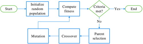
Genetic Algorithms are evolutionary computational algorithms generally applied to machine learning and problem optimization exploiting evolutionary principles like the survival of the fittest and mutation (Mirjalili 2019; Katoch et al. 2021). Figure 11 shows a basic example of this algorithm, where the main steps are presented as follows: a random population is first created where each individual carries values for each attribute or ’gene’; we promote the population evolution by firstly choosing the individuals that better solve the proposed problem or better fit to the evaluation metric; these individuals will create a new population offspring by combining a fraction of the parent’s genes, in the process called ’crossover’; then, the new population (or offspring) suffers a random mutation in its genes finishing the generation of a new population; finally, the process starts again by evaluating the population and choosing the best individuals.

Figure 11. Basic Genetic Algorithm workflow.

This approach differs from Artificial Neural Networks or other supervised learning algorithms by optimizing attributes in the desired solution model. We propose using GA in this work to optimize the parameters in Equation 7(7) $$\mathrm{ }\mathit{ACRI}=\frac{1}{D_2}\left(D_1-\left(\frac{{\rho }_1\cdot R_1-R_2\cdot {\rho }_2-T{x}^2}{C_1}\cdot \frac{{\rho }_2-T{y}^2}{C_2}\right)\right),$$(7) , creating individuals for our population set carrying the eight variables as genes ($T_1,$ $T_2,$ $R_1,$ $R_2,$ $C_1,$ $C_2,$ $D_1$ and $D_2$). The population is set to a number of 300 individuals, where the 20 best individuals, considering the $R^2$ score (shortly presented in the section following), will be the parents of the next offspring. The crossover step randomly takes 50% of the genes from each parent, while the mutation occurs in 40% (or 2 genes) of the resulting genes. The mutation in this case is the addition of a random value, either negative or positive, to the gene value in a stochastic manner. The genetic algorithm optimization is set to run for 1000 generations for each scenario.

To guarantee the performance and future usage over different outcrops, we organized the testing experiments by iteratively using small subsets as adaptation samples. We defined a standard sliding window with a representative size according to the image dimensions (about 20% of the image size) to collect all possible sampling scenarios and use it as input for tuning the index coefficients. A representation of the proportions between the sampling size against the whole image is given in Figure 9 (rectangle at upper left of each image color composition). The validation was always made using the entire image used as an example and the corresponding ground truth made by visual interpretation using HR data followed by resampling to the natural resolution of the image.

4.3. Results from the adaptive method

Performance of the index after adjusting coefficients $T_1,$ $T_2,$ $R_1,$ $R_2,$ $C_1,$ $C_2,$ $D_1$ and $D_2$ was tested and has shown interesting results. The new values were slightly different from the original ones, as can be seen in Table 2, which compares the coefficients initially found for Soledade (source domain) and the updated values found for Rosário and Furna Feia (target domains). The 3-dimensional surfaces after adjusting the index coefficients for each outcrop are shown in Figure 12. As can be seen, the general shape of the surface was preserved, whereas the position and other barely noticeable details were changed. However, the seemingly small changes were able to promote important improvements in the performance of the index for the new environments. As expected, Table 3 shows maximum, minimum, and mean values for validation metrics MAE, MSE, and $R^2$ larger than the ones found by using the original formulation (Table 1). The new scores also outperformed the other approaches used for comparison.

Figure 12. 3-dimensional index surface after adjusting coefficients by supervised genetic algorithm proposed. (a) Rosário and (b) Furna Feia. Viewing perspectives are fixed and the same as in Figure 8a.

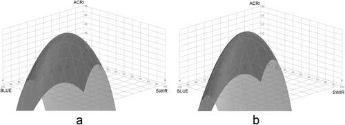
Table 2. Adaptive coefficients after convergence for source and target domains.

	$D_1$	$D_2$	$C_1$	$C_2$	$R_1$	$R_2$	$T_x$	$T_{y}$
Soledade (source)	25.0	65.0	600	23.0	2.45	2.10	74	28
Rosário (target)	22.3	61.2	512	21.7	2.28	2.31	62	31
Furna Feia (target)	26.1	63.7	591	22.8	2.63	2.29	67	26

Slight variations in values of coefficients are due to specific characteristics of the corresponding domains.

Table 3. ACRI after adaptation for Furna Feia and Rosario outcrops using the same 30 random executions of the 20% image window sampling. Lower mean values indicate better results.

	Furna Feia		Rosário
	Mean	Std	Mean	Std
MAE	0.174	0.026	0.161	0.014
MSE	0.057	0.014	0.043	0.008
R2	0.53	0.10	0.71	0.07.

All rates are better than any of the indices found in Table 1. The best rates are in boldface.

Figure 13 present the results for Rosário and Furna Feia outcrops after adaptation. Visual comparison between the reference image and the adaptive index depicted in Figure 13 can attest their similarity. Essentially, there are no substantial visual differences when compared with the previous results (before adaptation). However, the quantitative performance was considerably better than the first index scores.

Figure 13. Result generated after adaptation for Rosário and Furna Feia outcrops (target domains). Grey scale images vary from zero (no carbonates) to one (totally occupied by carbonates). Visual results are very similar to what was found in 13, however quality scores depicted in Table 3 show overall improvements.

5. Discussion

The performance of the proposed adaptive index is hardly dependent on the adaptation procedure. Therefore, after adaptation, the results are noticeably improved in all the reported experiments. To use unmixing models or other general indices that do not require a priori information is a convenient solution, but these approaches always have a baseline location (or a specific situation) where the formulation was developed and tested. Disturbances between different regions are capable to add noise to the results, which are only detected if the analyst has reliable ground truth data. Afterwards, developing a basic mathematical formulation that can be slightly adapted to similar situations can be more labor intensive. However, the outcome can greatly compensate for the additional work, since small gradients of sedimentary material can indicate directions of higher potential for oil content through the outcrop.

6. Conclusions

In this paper, we proposed an adaptive index based on spectral channels at visible and SWIR regions to indicate carbonate rocks in outcrop areas. In general, the spectral reflectance of natural targets is affected by multiple physical processes, and we could prove the difficulties to establish a unique solution able to produce optimal results for all applications everywhere and at all times. By using sample data from different sources, we developed an equation based on the best features selected using analysis assisted by reliable ground truth derived from field surveys and high spatial resolution UAV images. Thus, we used genetic optimization algorithm to fine-tuning the coefficients of the original equation in the adaptation stage. The experiments performed in the Soledade outcrop proved the effectiveness of the proposed equation against the six methods used for comparison (ACRI, KBRI, CRI1, CRI2, NDRI1, NDRI2, SLMM). Our experiments also evidenced that adaptation is needed to extend the index usage in different carbonate outcrops. The adaptation step involves a selection of a small subset of the image accompanied by an annotated ground truth made by visual interpretation. The genetic algorithm was able to adjust the coefficients of the original equation, which was attested by the improved performance verified at the Rosário and Furna Feia outcrops.

Disclosure statement

No potential conflict of interest was reported by the authors.

References

- Adelabu SA, Adepoju KA, Mofokeng OD. 2020. Estimation of fire potential index in mountainous protected region using remote sensing. Geocarto Int. 35(1):29–46.
- Alexander C. 2020. Normalised difference spectral indices and urban land cover as indicators of land surface temperature (LST). Int J Appl Earth Obs Geoinf. 86:102013.
- Arvor D, Durieux L, Andrés S, Laporte M-A. 2013. Advances in geographic object-based image analysis with ontologies: a review of main contributions and limitations from a remote sensing perspective. ISPRS J Photogramm Remote Sens. 82:125–137.
- Asadzadeh S, de Souza Filho CR. 2020. Characterization of microseepage-induced diagenetic changes in the Upper-Red Formation, Qom region, Iran. Part I: Outcrop, geochemical, and remote sensing studies. Mar Pet Geol. 117:104149.
- Baranwal E, Ahmad S, Mudassir SM. 2022. New independent component-based spectral index for precise extraction of impervious surfaces through Landsat-8 images. Geocarto Int. 34(10):1–29.
- Basso M, Kuroda MC, Vidal AC. 2017. Análise geológica e petrofísica de um bloco de travertino como análogo de reservatório de hidrocarbonetos. Geol USP Sér Cient. 17(2):211–221.
- Batista JE, Cabral AI, Vasconcelos MJ, Vanneschi L, Silva S. 2021. Improving land cover classification using genetic programming for feature construction. Remote Sensing. 13(9):1623.
- Bouhennache R, Bouden T, Taleb-Ahmed A, Cheddad A. 2019. A new spectral index for the extraction of built-up land features from Landsat 8 satellite imagery. Geocarto Int. 34(14):1531–1551.
- Cao Z, Cheng T, Ma X, Tian Y, Zhu Y, Yao X, Chen Q, Liu S, Guo Z, Zhen Q, et al. 2017. A new three-band spectral index for mitigating the saturation in the estimation of leaf area index in wheat. Int J Remote Sens. 38(13):3865–3885.
- Crowley JK. 1984. Multispectral remote sensing of carbonate rocks in the confusion range, Utah. In: Proceedings of the International Symposium on Remote Sensing of Environment, Third Thematic Conference: Remote Sensing for Exploration Geology. p. 837–851.
- de Linaje VA, Khan SD, Bhattacharya J. 2018. Study of carbonate concretions using imaging spectroscopy in the Frontier Formation, Wyoming. Int J Appl Earth Obs Geoinf. 66:82–92.
- Ford D, Williams PD. 2013. Karst hydrogeology and geomorphology. Chichester, UK: John Wiley & Sons.
- Fulcher J. 2008. Computational intelligence: an introduction. In: John Fulcher and L.C. Jain (Eds.). Computational intelligence: a compendium. Berlin, Heidelberg: Springer; p. 3–78.
- Genú AM, Roberts D, Demattê JAM. 2013. The use of multiple endmember spectral mixture analysis (mesma) for the mapping of soil attributes using aster imagery. Acta Sci Agron. 35(3):377–386.
- Govaerts YM, Verstraete MM, Pinty B, Gobron N. 1999. Designing optimal spectral indices: a feasibility and proof of concept study. Int J Remote Sens. 20(9):1853–1873.
- Huang Q, Cai Y. 2009. Mapping karst rock in southwest china. Mt Res Dev. 29(1):14–20.
- Huynh HH, Yu J, Wang L, Kim NH, Lee BH, Koh S-M, Cho S, Pham TH.,. 2021. Integrative 3d geological modeling derived from swir hyperspectral imaging techniques and uav-based 3d model for carbonate rocks. Remote Sensing. 13(15):3037.
- Katoch S, Chauhan SS, Kumar V. 2021. A review on genetic algorithm: past, present, and future. Multimed Tools Appl. 80(5):8091–8126.
- Lambora A, Gupta K, Chopra K. 2019. Genetic algorithm- a literature review. In: 2019 International Conference on Machine Learning, Big Data, Cloud and Parallel Computing (COMITCon); p. 380–384.
- Li S, Wu H. 2015. Mapping karst rocky desertification using Landsat 8 images. Remote Sensing Lett. 6(9):657–666.
- Malainine C-E, Raji O, Ouabid M, Khouakhi A, Bodinier J-L, Laamrani A, El Messbahi H, Youbi N, Boumehdi MA.,. 2022. An integrated aster-based approach for mapping carbonatite and iron oxide-apatite deposits. Geocarto Int. 37(22):6579–6601.
- Marques A, Horota RK, de Souza EM, Kupssinskü L, Rossa P, Aires AS, Bachi L, Veronez MR, Gonzaga L, Cazarin CL, et al. 2020. Virtual and digital outcrops in the petroleum industry: a systematic review. Earth-Sci Rev. 208:103260.
- Menezes DF, Bezerra FH, Balsamo F, Arcari A, Maia RP, Cazarin CL. 2020. Subsidence rings and fracture pattern around dolines in carbonate platforms – implications for evolution and petrophysical properties of collapse structures. Mar Pet Geol. 113:104113.
- Mirjalili S. 2019. Genetic algorithm. In: Seyedali Mirjalili (Ed.), Evolutionary algorithms and neural networks; p. 43–55. Berlin/Heidelberg, Germany: Springer.
- Muller M, Sales V, Zanotta DC, Marques A, Guimarães TT, Bachi L, et al. 2020. A quantitative analysis on different carbonate indicators based on spaceborne data in a controlled karst area. In: IGARSS 2020-2020 IEEE International Geoscience and Remote Sensing Symposium; p. 5207–5210.
- de Oliveira J, de Castro Manso CL, de Jesus Andrade E. 2013. Petalobrissus do cretáceo da formação jandaíra. Braz J Geol. 43(4):661–672.
- Oliveira J, Manso C, Andrade E, Souza-Lima W. 2013. O g^ênero mecaster (echinodermata: spatangoida) do cretáceo superior da formção jandaíra, bacia potiguar, nordeste do brasil. Sci Plena. 9(8):1–17.
- Pei J, Wang L, Huang N, Geng J, Cao J, Niu Z. 2018. Analysis of Landsat-8 oli imagery for estimating exposed bedrock fractions in typical karst regions of southwest china using a karst bare-rock index. Remote Sensing. 10(9):1321.
- Pessoa Neto O, Soares UM, Fernandes da Silva J, Roesner EH, Pires Florencio C, Valentin de Souza CV. 2007. Bacia potiguar. Bol geoci petrobras. 15(2):357–369.
- Piyoosh AK, Ghosh SK. 2022. Analysis of land use land cover change using a new and existing spectral indices and its impact on normalized land surface temperature. Geocarto Int. 37(8):2137–2159.
- Qu C, Li P, Zhang C. 2021. A spectral index for winter wheat mapping using multi-temporal Landsat ndvi data of key growth stages. ISPRS J Photogramm Remote Sens. 175:431–447.
- Rencz AN, Ryerson RA. 1999. Manual of remote sensing, remote sensing for the earth sciences. vol. 3. New York, USA: John Wiley & Sons.
- Saha SK. 2022. Remote sensing and geographic information system applications in hydrocarbon exploration: a review. J Indian Soc Remote Sens. 50(8):1457–1475.
- Shimabukuro YE, Smith JA. 1991. The least-squares mixing models to generate fraction images derived from remote sensing multispectral data. IEEE Trans Geosci Remote Sensing. 29(1):16–20.
- Silva OL, Bezerra FH, Maia RP, Cazarin CL. 2017. Karst landforms revealed at various scales using lidar and uav in semi-arid brazil: consideration on karstification processes and methodological constraints. Geomorphology. 295:611–630.
- Soares UM, Rosseti E, Cassab RCT. 2003. Bacias sedimentares brasileiras: bacia potiguar. Fundação Paleontol Phoenix. 56:1–5.
- Steinberg D. 2009. Cart: classification and regression trees. In: Xindong Wu, Vipin Kumar (Eds.). The top ten algorithms in data mining. Vol. 9; p. 179. New York: Chapman and Hall/CRC.
- Tangestani MH, Shayeganpour S. 2020. Mapping a lithologically complex terrain using Sentinel-2a data: a case study of Suriyan area, southwestern Iran. Int J Remote Sens. 41(9):3558–3574.
- Verstraete MM, Pinty B. 1996. Designing optimal spectral indexes for remote sensing applications. IEEE Trans Geosci Remote Sensing. 34(5):1254–1265.
- Verstraete MM, Pinty B, Myneni R. 1994. Understanding the biosphere from space: strategies to exploit remote sensing data. In: CNES, Proceedings of 6th International Symposium on Physical Measurements and Signatures in Remote Sensing.
- Xie X, Du P, Xia J, Luo J. 2015. Spectral indices for estimating exposed carbonate rock fraction in karst areas of southwest china. IEEE Geosci Remote Sens Lett. 12(9):1988–1992.
- Xue J, Su B. 2017. Significant remote sensing vegetation indices: a review of developments and applications. J Sens. 2017:1–17.
- Yang D, Chen J, Zhou Y, Chen X, Chen X, Cao X. 2017. Mapping plastic greenhouse with medium spatial resolution satellite data: development of a new spectral index. ISPRS J Photogramm Remote Sens. 128:47–60.
- Yue Y, Zhang B, Wang K, Liu B, Li R, Jiao Q, Yang Q, Zhang M. 2010. Spectral indices for estimating ecological indicators of karst rocky desertification. Int J Remote Sens. 31(8):2115–2122.
- Zaini N, Van der Meer FV, Van der Werff H. 2012. Effect of grain size and mineral mixing on carbonate absorption features in the SWIR and TIR wavelength regions. Remote Sensing. 4(4):987–1003.
- Zanotta DC, Haertel V, Shimabukuro YE, Renno CD. 2014. Linear spectral mixing model for identifying potential missing endmembers in spectral mixture analysis. IEEE Trans Geosci Remote Sensing. 52(5):3005–3012.
- Zheng Q, Huang W, Cui X, Shi Y, Liu L. 2018. New spectral index for detecting wheat yellow rust using Sentinel-2 multispectral imagery. Sensors. 18(3):868.