Applicability of SWOT data in calibrating WRF-Hydro hydrological model over the Tawa River basin

Abstract

Freshwater is considered an essential natural resource that must be monitored effectively. The Surface Water and Ocean Topography (SWOT) satellite mission scheduled for launch in December 2022 will enable river discharge estimation from surface water extents, elevations, and slopes. However, the SWOT-based discharges will be inconsistent due to infrequent temporal sampling (TS) of SWOT orbit. This study explores the potential of unique TS of SWOT to determine whether it influences the calibration of hydrological model. The Weather Research and Forecast Hydrological system (WRF-Hydro) has been used to simulate river discharge. Further WRF-Hydro model has been calibrated using proxy SWOT data based on a dynamically dimensioned search algorithm. Results show that more than 90% of parameter iterations have KGE values with less than 20% absolute percent difference when only SWOT TS alone has been considered. The results suggest that model calibration using SWOT-based discharge performs similarly to daily in-situ discharge.

Keywords:

• Satellite altimetry
• Surface Water and Ocean Topography (SWOT)
• WRF-hydro
• temporal sampling
• calibration

1. Introduction

Understanding the dynamics of river discharge is crucial for hydrological applications like water resource allocation and flood risk management (Jongman et al. 2012; Durand et al. 2014; Kansakar and Hossain 2016). Hydrological models such as Weather Research and Forecast Hydrological system (WRF-Hydro) have the potential to comprehend and access the transport of water, thereby serving applications like flood forecasting (Andreadis and Schumann 2014). In recent years, WRF-Hydro has expanded into a more versatile coupling architecture for integrating hydrological and atmospheric models. Coupled with fine-scale hydro-meteorological models, WRF-Hydro can estimate runoff, streamflow, and flood forecasts at grid resolutions of a few kilometers or less (e.g. (Yucel et al. 2015; Senatore et al. 2015; Arnault et al. 2016). However, parameter calibration of WRF-Hydro is crucial for accurately simulating the observed runoff process, including those governing the channel’s total water volume and discharge distribution. Hence, to ensure superior performance by hydrologic models, in-situ observations are quintessential for the calibration process, such as river discharge (Sun et al. 2012).

Unfortunately, quantifying in-situ discharge measurement is not possible for a variety of reasons, including the dispersed location of gauge stations (Vorosmarty et al. 2001) or owing to the lack of data sharing policy among the neighboring nations (Biancamaria et al. 2011; Hossain et al. 2014). The potential reason for scarcity in discharge measurements is sometimes lack of resources for the deployment of in-situ gauges (Hrachowitz et al. 2013), especially in ungauged basins or remote areas. Also, the nation’s contentious water policy results in a lack of measurement transparency (Gleason et al. 2018). Furthermore, the deployment of man-made obstructions such as dams have altered the natural flow regime of rivers to such an extent that the historical gauging stations, which had a more extended period of discharge measurement, are no longer applicable for analyzing current river dynamics (Pinter et al. 2008; Hossain et al. 2014; Wu et al. 2018). As a result, there is a need to investigate alternative ways of determining river discharge in addition to field measurements.

Remotely sensed satellite observations have a great advantage over in-situ observations in terms of spatial coverage and global accessibility (Alsdorf and Lettenmaier 2003). The remotely sensed satellite observations are not intended to replace in-situ gauge stations but rather to complement existing data collections (Alsdorf et al. 2003; Papa et al. 2010; Hossain et al. 2014; Thakur et al. 2021; Verma et al. 2021; Dhote et al. 2021). Unfortunately, neither a satellite nor an airborne sensor can directly measure the river discharge; rather, the river discharge can be estimated from remotely sensed hydrologic observables such as surface water extent and elevations (Bjerklie et al. 2003; Smith and Pavelsky 2008; Gleason and Smith 2014; Durand et al. 2016; Tarpanelli et al. 2017).

In the past two decades, satellite altimetry has shown great potential in observing surface water elevations, despite its limited spatial coverage due to its nadir look and 10- to 35-day revisit time (JASON and SARAL/AltiKa, respectively) (Verma and Indu 2021). Previous studies have tried to reduce the revisit cycles and spatial coverage of altimetry by combining multi-missions, but this further led to an additional challenge of bias correction of incongruent orbital cycles of different altimetry missions for observed space in time (Crétaux et al. 2015; Tarpanelli et al. 2017; Bjerklie et al. 2018). So, until the Surface Water and Ocean Topography (SWOT) mission, which was launched in December 2022, the desired requirement for studying surface water elevations and extent, along with enhanced sampling frequency by a single satellite was still distinct. Due to its wide swath of 120 km, the SWOT will globally observe both surface water elevation and extent (Biancamaria et al. 2016; Nair et al. 2022). The SWOT measurements such as river width, elevation, and slopes have been used to derive river discharge and associated uncertainties in many previous studies (Gleason and Smith 2014; Garambois and Monnier 2015; Durand et al. 2016; Bonnema and Hossain 2017; Hagemann et al. 2017), but very few studies analyzed the irregular Temporal Sampling (TS) of SWOT orbit (Nickles et al. 2020). Pedinotti et al. (2014) demonstrate how satellite remote sensing, coupled with hydrologic models, improves discharge estimation. Elmer et al. (2020) investigate how data assimilation is an alternative method for incorporating remotely sensed observations into models for discharge estimation, which would be important for SWOT-observed data. Huang et al. (2020) calibrated a hydrologic model using SWOT-like observations in ungauged basins and obtained a 0.85 Nash–Sutcliffe Efficiency. The study utilized Landsat-derived river widths and in-situ water levels to create SWOT observations. Even though these studies accurately represent SWOT-like observations, but they don’t examine whether SWOT's infrequent temporal sampling frequency would effectively perform hydrologic model calibration. So, the research is needed to identify the potential role of SWOT TS discharge versus daily discharge in calibrating hydrological models without data assimilation.

Even though the SWOT mission will enhance the spatial coverage, unlike current altimetry missions and in-situ gauge stations, SWOT observations are irregular (2 to 6 times observation) depending on the latitude within 21 days of the repeat orbit (Pavelsky et al., 2014)(Pavelsky et al. 2014). The present study examines the research hypothesis: “Will SWOT measurements be useful in hydrological model calibration to improve model performance? This study focuses on identifying the potential role of SWOT temporal sampled discharge relative to daily discharge in calibrating hydrological models. The objective is to determine whether irregular TS-based SWOT discharge may replace daily in-situ observed discharge in future WRF-Hydro hydrological model calibration.

2. Materials and methods

2.1. Study area

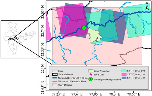
Tawa River is the longest (172 km) tributary of the Narmada River and drains through India’s Hoshangabad district of Madhya Pradesh state. Tawa dam is situated across the Tawa River at a latitude of 22⁰30’40” N and a Longitude of 77⁰56’30” E, which is a significant irrigation project in the state and covers a catchment area of about 6000 km² (Figure 1). The dominant soil type of the region is black alluvium and ferruginous red ravel, also called “black cotton.” The black-cotton soil has excellent porosity and moisture retention capability, making the region highly argillaceous. The region’s climatology can be majorly categorized into three seasons; pre-monsoon (March-April-May), post-monsoon (October-November-December), with nearly no rainfall, and monsoon (June-July-August-September), with an annual mean rainfall of about 550 mm. The monthly mean temperature ranges from 12° C (minimum temperature) to 42° C (maximum temperature). So, the water level of the Tawa dam provides crucial information to water managers to regulate the dam’s outflow, which is majorly dependent on the rainfall during the monsoon and inflows from the upstream river. In Figure 1, the WRF-Hydro domain (legend denoted as study domain) for the current study covers a large area of 65000 km², which also covers the streamflow of the tributaries coming from the east. Consequently, the output of the model at the Hoshangabad gauge station takes into account the flow of the large tributary flowing from the east. So, the model out at the Hoshangabad gauge station also considers the flow in tributary coming from the east. Also, the gauging station location corresponds to the outlet of the modeled watershed in the study.

Figure 1. Map of study area representing study domain, Hoshangabad gauge station location, SWOT calibration and validation orbital pass over the Narmada River.

2.2. Data used

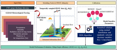
In the current study, in-situ observed daily discharge data at the Hoshangabad gauging station monitored by the Centre Water Commission (CWC) of India have been used from 1 January 2011 to 31 December 2017. Furthermore, for calibration, three types of discharge data have been used. First is the in-situ observed or gauge discharge data (hereinafter referred to as Q_g) downloaded from the Indian Water Resource Information System (India-WRIS) web portal. The second discharge data is based on the temporal revisit of SWOT (hereinafter mentioned as Q_gt), which is the subset of Q_g when the SWOT satellite passes over the gauging station. For the extraction of Q_gt from Q_g, the orbital pass and temporal cycle over the gauging station have been simulated using CNES Large-Scale Hydrology Simulator (https://github.com/CNES/swot-hydrology-toolbox). The third discharge data is SWOT-like data (Q_s) derived by following the Q_gt considering uncertainty associated with the SWOT discharge algorithm, defined in Hagemann et al. (2017).

2.3. WRF-Hydro model calibration

WRF-Hydro is fully distributed with multi-physics and multi-scale capabilities, enabling it to represent processes on various spatial scales (Yucel et al. 2015; Senatore et al. 2015; Arnault et al. 2016). The WRF-Hydro modeling system version 5.1.1 has been used in the study. The WRF-Hydro system contains several components of the distributed hydrological process and channel flow (Lahmers et al. 2019). WRF-Hydro and Noah-MP exhibit parameters often remain dependent on land use (i.e. vegetation density and type) and soil type (i.e. silt, clay, loam, sand). The calibration process determines the optimal coefficient values applied to parameters in the spatial domain. As suggested by Yucel et al. 2015; Verri et al. 2017; Rummler et al. 2019; Camera et al. 2020, four parameters that are most sensitive to discharge were calibrated namely: (i) soil permeability or runoff infiltration (REFKDT), (ii) surface retention depth (RETDEPRTFAC), (iii) overland flow roughness factor or surface runoff (OVROUGHTFAC), and (iv) Manning’s factor for channel roughness (MannN). The reference values have been provided in Table 1.

Table 1. WRF-Hydro calibration parameter, definition, and scaling factor ranges considered in calibration process.

Parameter	Definition	Range of parameter value	Reference parameter value	Calibrated parameter values
				for Qg	for Qgt	for Qs
REFKDT	Runoff infiltration	0.5-1.5	0.50	1.20	1.26	1.35
RETDEPRTFAC	Surface retention depth	0-10	1.00	4.50	3.29	3.20
OVROUGHRTFAC	Surface roughness	0.1-1	1.00	0.59	0.54	0.53
Manning’s roughness	Channel roughness	0.5-0.00125	0.40	0.03	0.03	0.02

The calibration procedure is based on the Dynamically Dimensioned Search (DDS) algorithm designed by Tolson and Shoemaker (2007). The DDS is a simple, heuristic, single-solution-based global search algorithm developed to find approximated globally optimal solutions within the specified range of function evaluations (Tolson and Shoemaker 2007). The algorithms start with the global search and gradually progress towards the local search while approaching a maximum allowable number of the model iterations. The gradual transition from global to local search exhibits dynamic adjustment to the search dimension, and the parameters’ dimensionality changes. The algorithm randomly selects the parameters with the best solution of the current model iteration and slightly distributes them to generate a revised candidate solution in the next iteration. DDS is, therefore, not designed to cover the global optimum precisely; however, it covers the regional global optimum in the best case and good local optimum in the worst-case scenarios (Tolson and Shoemaker 2007).

For the experiment, model iteration has been performed using a combination of four parameter values chosen by the DDS algorithm within the predefined range tabulated in Table 1. The error matric in each iteration has been calculated by comparing the WRF-Hydro model output (Q_w) with Q_g, Q_gt, and Q_s, respectively. The aim is to see the impact on the model calibration with respect to different discharge time series concerning infrequent TS of the SWOT mission. Since the SWOT mission’s planned designed life is for three years, calibration of WRF-Hydro model simulations have been performed from the year 2015 to 2017 with one year of model spin-up. WRF-Hydro model output was calibrated at the Hoshangabad gauge station, which had consistent daily data from 2011 to 2017. Furthermore, to access the performance of each set of parameters, Kling-Gupta efficiency (KGE) (Gupta et al. 2009) has been calculated between the Q_w and each of three time-series (Q_g, Q_gt, and Q_s) respectively (Figure 2). Where, the KGE is defined in Equation 1(1) $$\mathit{KGE}=1-\mathrm{ }\sqrt{{\left(r-1\right)}^2{+\left(\beta -1\right)}^2+{\left(\gamma -1\right)}^2}$$(1) . (1) $$\mathit{KGE}=1-\mathrm{ }\sqrt{{\left(r-1\right)}^2{+\left(\beta -1\right)}^2+{\left(\gamma -1\right)}^2}$$(1)

Figure 2. Methodology flowchart for calibrating WRF-Hydro model using DDS algorithm.

Where; $r=\mathrm{ }\frac{\mathit{cov}\left(Q_m,Q_o\right)}{{\sigma }_{Q_m}{\sigma }_{Q_o}};\mathrm{ }\beta =\mathrm{ }\frac{{\mu }_{Q_m}}{{\mu }_{Q_o}};\mathrm{ }\gamma =\mathrm{ }\frac{{\sigma }_{Q_m}/{\mu }_{Q_m}}{{\sigma }_{Q_o}/{\mu }_{Q_o}}$

Where r is the correlation coefficient, β is the bias ratio, and γ is the relative variability between the time series such Q_w and one of three times series (Q_g, Q_gt, and Q_s). Also, µ, and σ denotes the mean and standard deviation of the time series. A KGE value closer to 1 represent the model output accuracy with respect to the in-situ value (Knoben et al. 2019).

The entire watershed contained shallow to medium-depth alluvium formations, both recent and old. The dominant soil type of the region is black alluvium and ferruginous red ravel, also called “black cotton.” The black-cotton soil has excellent porosity and moisture retention capability, making the region highly argillaceous. The study area is located in the north, and forest cover can be seen along the foothills of India’s Satpura range. The slope is generally steep in the foothills of the Satpura range but moderate to gentle towards the Narmada River (Malik and Shukla 2015). Because of good irrigation sources and fertile alluvial soil, the entire catchment area is rich in agriculture. Agricultural land accounts for nearly 90% of the watershed basin’s total area. The Satpura range’s foothills are covered in forest. There are also some patches of scrub land near both banks of the Tawa River (Malik and Shukla 2015). This land use and land cover class may greatly influence the MannN parameter. Based on previous studies, Chen (2007) has suggested that the REFKDT parameter controls the hydrograph volume. Also, the increment in the REFKDT factor by 0.1 considerably impacts the surface runoff.

Similarly, the REFKDT range in the current study is also considered from 0.5 to 1.5 with an increment factor of 0.1. Hence, it was anticipated that the infiltration and surface retention depth were more sensitive to KGE values than other parameters. In the WRF-Hydro modeling system, the available streamflow input water is derived mainly from the amount of precipitation in infiltration capacity excess in each model grid (Ryu et al. 2017). It can also be inferred from (Dubey et al. 2021) that when soil condition is unsaturated, higher is the REFKDT value and smaller is the simulated volume. Also, the increment in REFKDT decreases surface runoff. This supports the assertion that REFKDT values are significantly high when the soil is unsaturated during non-monsoon or low-flow conditions.

3. Results and discussion

The WRF-Hydro parameters and corresponding relationship with KGE values have been shown in Figure 3. In Figure 3, we can see that the best model iteration based on optimal parameters was selected by the DDS algorithm concerning different target discharge Q_g in Figure 3(a), Q_gt in Figure 3(b), and Q_s in Figure 3(c) during the calibration stage. The DDS algorithm arbitrarily selected the initial parameter values during the global search phase. However, as the number of iterations increased, the negative KGE values improved during the local search phase, along with the reduction in the randomness of parameters.

Figure 3. WRF-Hydro model calibration performance using KGE for different normalized parameter values obtained by the best iteration of the DDS algorithm targeting the different discharge: (a) Q_g, (b) Q_gt, and (c) Q_s. The x-axis represents the best model iteration, the left vertical axis represents the model performance by KGE, and the right vertical axis represents the normalized values of parameters selected by the DDS algorithm for calibrating the model. The normalized values of parameters have been shown to represent better parameter values having varied scales.

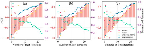
The parameters such as surface infiltration (REFKDT) and surface retention depth (RETDEPRTFAC) are more sensitive towards the KGE than other parameters. In Figure 3(a), the slight variation of a 0.07 scaling factor in surface retention depth and a 2-scaling factor change in surface infiltration impact KGE values ranging from −1 to 0.65 by 24 model iterations. It can be observed that when the soil is unsaturated during non-monsoon or low-flow conditions, the REFKDT values are much higher. However, with the increment in the REFKDT scaling factor, the hydrograph becomes much smoother due to a decrease in surface runoff which further affect the KGE values. Similarly, the roughness parameters such as OVROUGHRTFAC and MannN control the speed of streamflow in the channel network. The MannN parameter scaling factor’s linear increment increases the KGE values. However, the OVROUGHRTFAC parameter scaling factor decreases the KGE values due to the prolonged confluence time of surface runoff. In Figure 3(b), since the Q_gt has been derived from Q_g, it can be observed that the comparison between the model calibration based on Q_g and Q_gt has no significant difference in normalized parameter range and KGE values. However, the model calibration based on Q_s has a slight skewness in the KGE values towards the right (Figure 3c). Also, a slight discrete pattern in parameter selection has been observed during the local search of the DDS algorithm. So, it can be observed that the calibration targeting Q_g derived from infrequent TS of SWOT has no significant effect on optimizing best parameters in fewer model iterations than Q_s. Also, the calibration performance of Q_gt in terms of KGE values was found to be better than Q_s. Overall, the DDS algorithm has converged the parameter values to the best performance level of KGE at the Hoshangabad gauge station shown in Table 1.

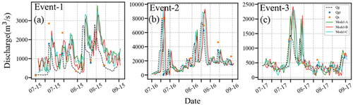
Further, the WRF-Hydro model iteration comparison with the time series has been shown in Figure 4. Figure 4 represents discharges simulated by WRF-Hydro based on the best parameters selected by the DDS algorithm. Figure 4 shows three Events over three years (from 2015 to 2017). In each event, the comparison was made between the true discharge value and the model outputs (Model-A, Model-B, and Model-C). Model-A represents the discharge time series based on the optimal calibrated parameter targeting the discharge Q_g (true discharge). Model-B represents the discharge time series based on the optimal calibrated parameter targeting the discharge Q_gt (which is a temporally sampled sub-set of Q_g). And, Model-C represents the discharge time series based on the optimal calibrated parameter targeting the discharge Q_s (same as Q_gt but associated with discharge uncertainty). Since the SWOT mission was designed for three years, the WRF-Hydro model calibration was evaluated from 2015 to 2017. The intercomparison of different discharges during extreme events each year is shown in Figure 4. The intercomparison of different discharges was carried out during the peak flows. It was observed from Figure 4 that for all three events, Model-A, Model-B, and Model-C have captured the streamflow dynamics. For Event-1, Model-A, Model-B, and Model-C were able to capture the streamflow dynamics but with consistent lag. The potential reason for having the consistent lag may be due to MannN parameter values for all the models. Also, the increase in runoff infiltration affects the occurrence of the peak. In the previous studies, Liu et al. (2021) and Dubey et al. (2021), It has been shown that when the value of REFKDT is increased by 0.5, the peak time is delayed by approximately two hours. In the current study, the REFKDT value was ranging from 0.5 to 1.5, with an increment factor of 0.5. Hence, a time lag has been observed. The MannN parameter may have a significant impact on the transit time of the streamflow. The lower the value of MannN, the faster the transit time and, as a result, the higher discharge. It should also be noted that the MannN parameter collaborates closely with REFKDT to influence the simulated hydrograph. Another potential reason for the time lag could be the outflow from the Tawa dam. The Tawa dam, which is in the study domain, covers 3600 grid points. But the reservoir was not modeled in this study due to the unavailability of outflow data from the reservoir. So, the unmodelled reservoir outflow in the channel routing shows the time lag. So, during Event-1 (Figure 4(a)), in which the maximum flow reaches up to 3000 m³/s, Model-A, Model-B, and Model-C have overestimated the discharge with respect to Q_g. However, during the Event 2 (Figure 4(b)), the peak flow was up to 10000 m³/s. The Model-A, Model-B, and Model-C were able to capture high flow dynamics quite accurately but again overestimated the Eevent-3 when the peak went down to 1500 m³/s. The potential reason for capturing the high peaks by the model would be the objective function KGE, for which the model calibration has been optimized. So, it can be stated that all the models perform well during the high flow or monsoon season compared to low flow. Further, the WRF-Hydro model calibration based on Model-B has similar results as Model-A and Model-C. So, it has been observed that the performance of all models is different for different even though the underlying data used (i.e. a subset from the in-situ discharge data) remains the same.

Figure 4. Calibration of discharge with optimized Model-A, Model-B, and Model-C parameters for the (a) Event -1, (b) Event-2, and (c) Event-3 at Hoshangabad gauge station.

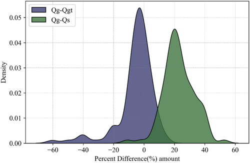
In the case of TS alone, Figure 5 shows that taking the area under the curve between ± 20% denotes that more than 90% of iterations have less than 20% absolute difference between Q_g and Q_gt (similar to Nickles et al. (2020). However, after combining the effect of TS with associated uncertainty, 60% of iteration shows less than 20% absolute difference between Q_g and Q_s. Furthermore, the density curve is skewed toward the right and has the most percentage difference toward positive values for Q_g-Q_gt and Q_g-Q_s. The density curve’s skewness indicates that comparing the Q_w with Q_g and Q_gt gives more positive KGE than Q_s. Since the Q_gt is derived from Q_g and has no uncertainty, It is expected to have more positive KGE in the case of Q_g-Q_gt compared to Q_g-Q_s.

Figure 5. Density curve of the percentage difference between time series Q_g-Q_gt and Q_g-Q_s. The density curve having an area equal to one represents the effect of SWOT TS alone (Q_g-Q_gt) and when combined with the uncertainty associated (Q_g-Q_s) over the KGE values in each iteration. The outlier has not been shown.

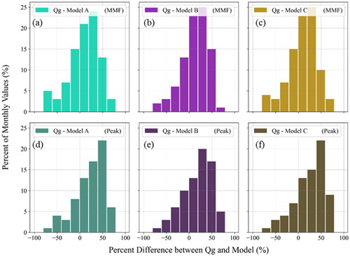
Based on the highest KGE values, the best parameter iterations were selected, and it was observed that the Q_gt more often performed well with Q_g than Q_w. To understand the difference in the performance of KGE values for Q_gt vs. Q_w and Q_g vs. Q_w, it is important to understand the formation of different discharge time series under comparison. Hence, the daily discharge time series have been considered while comparing Q_g vs. Q_w. However, the infrequent temporally sampled discharge has been considered in comparing Q_gt vs. Q_w. Since the model output matches well with the in-situ observed discharge values during the low flow and peak events (Figure 6), it is admissible that Q_gt vs. Q_w would provide better KGE values compared to KGE values obtained from Q_g vs. Q_w. Since the model calibration based on Q_g produces more robust model parameters, the improvement in KGE values alone from Q_gt does not necessarily represent the model performance (Nickles et al. 2020). Hence, it was observed that the Q_gt gives better KGE values and represents the monthly peak flow values even though only infrequent temporally sampled SWOT-based discharge has been selected. Contrarily, the Q_s were shown lower KGE values due to the combined effect of infrequent TS and uncertainty with a Gaussian error, which indicates a negative bias with a significant deviation or spread.

Figure 6. Histogram of the percentage difference between Q_g and monthly mean flow (MMF) i.e. (a) Qg-Model A, (b) Qg-Model B, (c) Qg-Model C and monthly peak flow i.e. (d) Qg-Model A, (e) Qg-Model B, (f) Qg-Model C for 2015-2017.

The Tawa Dam has influenced the natural water flow in the Narmada river basin, which further affects the hydrological model calibration. The WRF-Hydro hydrological model considers the dam as a natural lake and compensates for the flow mainly due to the dam’s unavailability of flow regulation data. Furthermore, the reservoirs may also affect the river’s flow due to significant evaporation loss, which further affects the calibration. However, irrespective of the hydrological model used, we have focused on the influence of infrequent SWOT-based discharge in the calibration parameters in this study. Also, the hydrological model performance may differ with different models and atmospheric forcing, and the current study is based on the calibration uncertainty in using different time series among Q_g, Q_gt, and Q_s.

4. Conclusions

The WRF-Hydro model calibration using discharge derived from the infrequent TS of SWOT has not been significantly different from daily in-situ discharge. Moreover, the SWOT-based discharge sometimes performed well than the daily in-situ discharge. On analyzing the DDS calibration iterations, it has been observed that the more than 90% of parameter iterations have KGE values with less than 20% absolute percent difference when only SWOT TS alone has been considered. Furthermore, the monthly mean and maximum flow values at the Hoshangabad gauge station have an average percentage difference of less than 10% for the best parameter iteration. These minor differences suggest that the WRF-Hydro hydrological model performance does not vary much by either calibrating using SWOT-based discharge or daily in-situ discharge. Even though the SWOT has infrequent TS and likely uncertainty, the SWOT-discharge-based calibrated hydrological model performed well in capturing the peaks and low values of discharge. This study suggests that the SWOT-based discharge helps calibrate the hydrological model when no in-situ flow information is available. This study will help downstream stakeholders to understand and monitor the catchment using hydrological modeling and SWOT data when upstream flow regulation information is limited. The results of the current study may vary with the use of the different hydrological models and atmospheric forcing data. However, further study is needed to investigate flood event forecasting based on calibration using infrequent temporally sampled SWOT discharge data.

Acknowledgements

Authors thank the support through DST CNRS project (DSTCNRS/2018-19-01/109) and the support through DST Centre of Excellence in Climate Studies, IIT Bombay through project DST/CCP/CoE/140/2018(G).

Disclosure statement

No potential conflict of interest was reported by the authors.

References

- Alsdorf D, Lettenmaier D, Vörösmarty C. 2003. The need for global, satellite-based observations of terrestrial surface waters. Eos Trans AGU. 84(29):269–276.
- Alsdorf DE, Lettenmaier DP. 2003. Tracking fresh water from space. Science. 301(5639):1491–1494.
- Andreadis KM, Schumann GJ-P. 2014. Estimating the impact of satellite observations on the predictability of large-scale hydraulic models. Adv Water Resour. 73:44–54.
- Arnault J, Wagner S, Rummler T, Fersch B, Bliefernicht J, Andresen S, Kunstmann H. 2016. Role of runoff–infiltration partitioning and resolved overland flow on land–atmosphere feedbacks: a case study with the WRF-hydro coupled modeling system for West Africa. J Hydrometeorol. 17(5):1489–1516.
- Biancamaria S, Hossain F, Lettenmaier DP. 2011. Forecasting transboundary river water elevations from space: river water height forecast from space. Geophys Res Lett. 38(11):L11401.
- Biancamaria S, Lettenmaier DP, Pavelsky TM. 2016. The SWOT mission and its capabilities for land hydrology. Surv Geophys. 37(2):307–337.
- Bjerklie DM, Birkett CM, Jones JW, Carabajal C, Rover JA, Fulton JW, Garambois P-A. 2018. Satellite remote sensing estimation of river discharge: application to the Yukon River Alaska. J Hydrol. 561:1000–1018.
- Bjerklie DM, Lawrence Dingman S, Vorosmarty CJ, Bolster CH, Congalton RG. 2003. Evaluating the potential for measuring river discharge from space. J Hydrol. 278(1–4):17–38.
- Bonnema M, Hossain F. 2017. Inferring reservoir operating patterns across the Mekong Basin using only space observations: reservoir behavior in the Mekong river. Water Resour Res. 53(5):3791–3810.
- Camera C, Bruggeman A, Zittis G, Sofokleous I, Arnault J. 2020. Simulation of extreme rainfall and streamflow events in small Mediterranean watersheds with a one-way-coupled atmospheric–hydrologic modelling system. Nat Hazards Earth Syst Sci. 20(10):2791–2810.
- Chen F. 2007. The Noah land surface model in WRF: a short tutorial. In: NCAR, LSM group meeting. http://www.atmos.illinois.edu/∼snesbitt/ATMS597R/notes/noahLSM-tutorial.pdf
- Crétaux J-F, Biancamaria S, Arsen A, Bergé-Nguyen M, Becker M. 2015. Global surveys of reservoirs and lakes from satellites and regional application to the Syrdarya river basin. Environ Res Lett. 10(1):015002.
- Dhote PR, Bansal J, Garg V, Thakur P, Agarwal A. 2021. Potential of multi-mission satellite altimetry observations and hydrodynamic model to establish virtual gauging network in sparsely Gauged Basin [Internet]. ESS Open Archive: Hydrology. 2021:H55A-0750.
- Dubey AK, Kumar P, Chembolu V, Dutta S, Singh RP, Rajawat AS. 2021. Flood modeling of a large transboundary river using WRF-Hydro and microwave remote sensing. J Hydrol. 598:126391.
- Durand M, Gleason CJ, Garambois PA, Bjerklie D, Smith LC, Roux H, Rodriguez E, Bates PD, Pavelsky TM, Monnier J, et al. 2016. An intercomparison of remote sensing river discharge estimation algorithms from measurements of river height, width, and slope: SWOT discharge algorithm intercomparison. Water Resour Res. 52(6):4527–4549.
- Durand M, Neal J, Rodríguez E, Andreadis KM, Smith LC, Yoon Y. 2014. Estimating reach-averaged discharge for the River Severn from measurements of river water surface elevation and slope. J Hydrol. 511:92–104.
- Elmer NJ, Hain C, Hossain F, Desroches D, Pottier C. 2020. Generating proxy SWOT water surface elevations using WRF‐hydro and the CNES SWOT hydrology simulator. Water Resour Res. 56(8).
- Garambois P-A, Monnier J. 2015. Inference of effective river properties from remotely sensed observations of water surface. Adv Water Resour. 79:103–120.
- Gleason CJ, Smith LC. 2014. Toward global mapping of river discharge using satellite images and at-many-stations hydraulic geometry. Proc Natl Acad Sci USA. 111(13):4788–4791.
- Gleason CJ, Wada Y, Wang J. 2018. A hybrid of optical remote sensing and hydrological modeling improves water balance estimation: water balance from remote sensing. J Adv Model Earth Syst. 10(1):2–17.
- Gupta HV, Kling H, Yilmaz KK, Martinez GF. 2009. Decomposition of the mean squared error and NSE performance criteria: implications for improving hydrological modelling. J Hydrol. 377(1-2):80–91.
- Hagemann MW, Gleason CJ, Durand MT. 2017. BAM: Bayesian AMHG-manning inference of discharge using remotely sensed stream width, slope, and height: BAM flow using stream width slope height. Water Resour Res. 53(11):9692–9707.
- Hossain F, Siddique-E-Akbor AH, Mazumder LC, ShahNewaz SM, Biancamaria S, Lee H, Shum CK. 2014. Proof of concept of an altimeter-based river forecasting system for transboundary flow inside Bangladesh. IEEE J Sel Top Appl Earth Observations Remote Sensing. 7(2):587–601.
- Huang Q, Long D, Du M, Han Z, Han P. 2020. Daily continuous river discharge estimation for ungauged basins using a hydrologic model calibrated by satellite altimetry: implications for the SWOT mission. Water Resour Res [Internet]. 56(7). [accessed 23 May 2022].
- Hrachowitz M, Savenije HHG, Blöschl G, McDonnell JJ, Sivapalan M, Pomeroy JW, Arheimer B, Blume T, Clark MP, Ehret U, et al. 2013. A decade of Predictions in Ungauged Basins (PUB)—a review. Hydrol Sci J. 58(6):1198–1255.
- Jongman B, Ward PJ, Aerts JC. 2012. Global exposure to river and coastal flooding: Long term trends and changes. Global Environ Change. 22(4):823–835.
- Kansakar P, Hossain F. 2016. A review of applications of satellite earth observation data for global societal benefit and stewardship of planet earth. Space Policy. 36:46–54.
- Knoben WJM, Freer JE, Woods RA. 2019. Technical note: inherent benchmark or not? Comparing Nash–Sutcliffe and Kling–Gupta efficiency scores. Hydrol Earth Syst Sci. 23(10):4323–4331.
- Lahmers TM, Gupta H, Castro CL, Gochis DJ, Yates D, Dugger A, Goodrich D, Hazenberg P. 2019. Enhancing the structure of the WRF-hydro hydrologic model for semiarid environments. J Hydrometeorol. 20(4):691–714.
- Liu S, Wang J, Wei J, Wang H. 2021. Hydrological simulation evaluation with WRF-Hydro in a large and highly complicated watershed: the Xijiang River basin. J Hydrol: Reg Stud. 38(100943).
- Malik MS, Shukla JP. 2015. Hydrogeological study of Tawa watershed basin of Hoshangabad District M.P India, with special reference to increase the groundwater potentiality of the region. Int. J. Sci. Eng. Appl. Sci. 1(9):11.
- Nair AS, Verma K, Karmakar S, Ghosh S, Indu J. 2022. Exploring the potential of SWOT mission for reservoir monitoring in Mahanadi basin. Adv Space Res. 69(3):1481–1493.
- Nickles C, Beighley E, Feng D. 2020. The applicability of SWOT’s non-uniform space–time sampling in hydrologic model calibration. Remote Sens. 12(19):3241.
- Papa F, Prigent C, Aires F, Jimenez C, Rossow WB, Matthews E. 2010. Interannual variability of surface water extent at the global scale, 1993–2004. J Geophys Res. 115(D12):D12111.
- Pavelsky TM,Durand MT,Andreadis KM,Beighley RE,Paiva RC,Allen GH,Miller ZF. 2014. Assessing the potential global extent of SWOT river discharge observations. J Hydrol. 519:1516–1525..
- Pedinotti V, Boone A, Ricci S, Biancamaria S, Mognard N. 2014. Assimilation of satellite data to optimize large-scale hydrological model parameters: a case study for the SWOT mission. Hydrol Earth Syst Sci. 18(11):4485–4507.
- Pinter N, Jemberie AA, Remo JW, Heine RA, Ickes BS. 2008. Flood trends and river engineering on the Mississippi River system. Geophys Res Lett. 35(23).
- Rummler T, Arnault J, Gochis D, Kunstmann H. 2019. Role of lateral terrestrial water flow on the regional water cycle in a complex terrain region: investigation with a fully coupled model system. J Geophys Res Atmos. 124(2):507–529.
- Ryu Y, Lim Y-J, Ji H-S, Park H-H, Chang E-C, Kim B-J. 2017. Applying a coupled hydro-meteorological simulation system to flash flood forecasting over the Korean Peninsula. Asia-Pacific J Atmos Sci. 53(4):421–430.
- Senatore A, Mendicino G, Gochis DJ, Yu W, Yates DN, Kunstmann H. 2015. Fully coupled atmosphere-hydrology simulations for the central Mediterranean: impact of enhanced hydrological parameterization for short and long time scales: fully coupled atmosphere-hydrology model. J Adv Model Earth Syst. 7(4):1693–1715.
- Smith LC, Pavelsky TM. 2008. Estimation of river discharge, propagation speed, and hydraulic geometry from space: Lena River, Siberia: river discharge and hydraulic geometry. Water Resour Res [Internet]. 44(3). [accessed 2022 May 23].
- Sun W, Ishidaira H, Bastola S. 2012. Calibration of hydrological models in ungauged basins based on satellite radar altimetry observations of river water level: calibration of hydrological models using radar altimetry observations. Hydrol Process. 26(23):3524–3537.
- Tarpanelli A, Amarnath G, Brocca L, Massari C, Moramarco T. 2017. Discharge estimation and forecasting by MODIS and altimetry data in Niger-Benue River. Remote Sens Environ. 195:96–106.
- Thakur PK, Garg V, Kalura P, Agrawal B, Sharma V, Mohapatra M, Kalia M, Aggarwal SP, Calmant S, Ghosh S, et al. 2021. Water level status of Indian reservoirs: a synoptic view from altimeter observations. Adv Space Res. 68(2):619–640.
- Tolson BA, Shoemaker CA. 2007. Dynamically dimensioned search algorithm for computationally efficient watershed model calibration: dynamically dimensioned search algorithm. Water Resour Res [Internet]. 43(1). [accessed 2022 May 23].
- Verma K, Indu J. 2021. Effect of satellite altimetry sampling error in estimating reservoir storage and outflow. Geocarto Int. 37(25):7580–7590.
- Verma K, Nair AS, Jayaluxmi I, Karmakar S, Calmant S. 2021. Satellite altimetry for Indian reservoirs. Water Sci Eng. 14(4):277–285.
- Verri G, Pinardi N, Gochis D, Tribbia J, Navarra A, Coppini G, Vukicevic T. 2017. A meteo-hydrological modelling system for the reconstruction of river runoff: the case of the Ofanto river catchment. Nat Hazards Earth Syst Sci. 17(10):1741–1761.
- Vorosmarty C, Askew A, Grabs W, Barry RG, Birkett C, Doll P, Goodison B, Hall A, Jenne R, Kitaev L, et al. 2001. Global water data: A newly endangered species. Eos Trans AGU. 82(5):54–54.
- Wu B, Zeng H, Yan N, Zhang M. 2018. Approach for estimating available consumable water for human activities in a river basin. Water Resour Manage. 32(7):2353–2368.
- Yucel I, Onen A, Yilmaz KK, Gochis DJ. 2015. Calibration and evaluation of a flood forecasting system: utility of numerical weather prediction model, data assimilation and satellite-based rainfall. J Hydrol. 523:49–66.