Assessing the accuracy of sensitivity analysis: an application for a cellular automata model of Bogota’s urban wetland changes

Abstract

This study analyzes the outcomes of Cellular Automata (CA) with different neighborhood sizes and spatial resolution configurations on the performance of the Future Land Use Simulation (FLUS) model. The analysis is executed using three analogic images to extract the land use/land cover in Bogota, Colombia, for three years: 1998, 2004, and 2010. The FLUS model has an Artificial Neuronal Network model, which was used for calculating the relationships between the land uses and the associated drivers and to estimate the probability of occurrence of each land use. Whenever a CA is used to model and simulate, sensitivity analysis (SA) becomes a crucial step in CA modeling to understand better the influence of parameters’ changes in the simulation outcomes. Therefore, the SA is conducted by varying the neighborhood sizes between 3 × 3, 5 × 5, and 7 × 7 for 5 and 30 meters. In addition, cross-classification maps, Area Under the Curve (AUC) of the Total Operating Characteristic, landscape metrics, the figure of merit, Fuzzy Kappa, and disagreement metrics were calculated to assess how well the model performed. High AUC values and low disagreement results show that, in general, the model performed well, and the accuracy of the outputs improves with a 3 × 3 neighborhood size and 5 meters spatial resolution. This study provides a broad assessment approach to the different methods that must be considered to evaluate the sensitivity of CA models in the simulation of urban wetlands’ spatial-temporal evolution.

Keywords:

• urban wetlands
• Cellular Automata (CA)
• sensitivity analysis
• Land use/land cover change
• FLUS model

1. Introduction

Land use and land cover changes (LUCC) are complex and dynamic, with non-linear fluctuations over time and various processes operating at different spatial and temporal scales (Vliet Wallentin and Neuwirth 2017). As a result, land change models using Cellular Automata (CA) are increasingly used to explore their dynamics and are considered as a foundation for public policy decisions. As a consequence, they should be submitted to a Sensitivity Analysis (SA) for exploring “what if” scenarios. In CA models, one can represent the spatial complexity and dynamics of LUCC by selecting various configurations of its essential elements, such as the neighborhood size and spatial resolution.

Studies on SA have shown that the variation in the model output can be apportioned to different sources of variations and that models’ outputs depend upon the information fed into them (Crosetto et al. 2000). Among different parameters tested in a SA, the literature reports different neighborhood sizes, types, and spatial resolution configurations in land-change models. Kocabas and Dragicevic (2006) conducted a SA by systematically varying the neighborhood size and type. Shafizadeh-Moghadam et al. (2017) evaluated the effects of varying spatial neighborhood sizes on the predictive performance of the Land Transformation CA Model. Varga et al. (2019) executed a SA to see how the size of the spatial filter in a CA model influences the outputs in a CA-Markov land change model applied in Hungary. Wang et al. (2021) explored different smoothed transition rules and neighborhood sizes to understand how they impact the outputs in an urban growth simulation.

Along the process of a SA, the assessment of the results phase becomes essential. Researchers have used different approaches to evaluate how well the models perform due to the variation of different model parameters. Many scientific articles have described the implementation of qualitative and quantitative methods. Kocabas and Dragicevic (2006) proposed assessing SA using a cross-classification map, Kappa index with coincidence matrices, and different spatial metrics. Shafizadeh-Moghadam et al. (2017) followed the metrics figured of merit (FoM), producer’s accuracy (PA), and overall accuracy (OA) indices. Wang et al. (2021) used five indicators: OA, Kappa coefficient, FoM, PA, and user’s accuracy (UA). Feng et al. (2022) applied cell-to-cell comparison techniques such as OA, PA, and UA in studying urban growth dynamics. When applying the previous methods, the sensitivity evaluation of the models showed that the neighborhood configuration affects the simulation quality. When applied in land-change models, smaller neighborhoods result in more accurate simulations.

Some researchers evaluated the model’s results by applying metrics that provided more profound insights. For example, the area under the curve (AUC) of the Total Operating Characteristic (TOC) curves is used to determine the accuracy of the models in the study of Kantakumar et al. (2020). Also, other articles like Tong and Feng (2019) suggest methods for evaluating model sensitivity, including the TOC. In addition, Pontius and Millones (2011a) proposed the use of two parameters: quantity disagreement (QD) and allocation disagreement (AD), which have been adopted to carry out the accuracy assessment of diverse simulation models of complex systems (Gaudreau et al. 2016; Islam et al. 2018; Tiné et al. 2019). These metrics are highly recommended in the literature thanks to their power to analyze the model in terms of error location and error quantity, offering more insights about what path to take to improve the simulation outcomes.

Since the SA and its assessment are fundamental during the calibration process of the model, it is necessary to apply and adopt a collection of evaluation methods in the pre-calibration stage of the model-building process. In research as in Kocabas and Dragicevic (2006), it is well documented a detailed and systematic SA assessment of a proposed CA model. Nevertheless, since the date of their publication, new techniques for evaluating SA in CA models have advanced; thus, it has become crucial to expand the documentation thus far. To do it, we have made a comprehensive literature review and chosen the analysis techniques more used and recommended within the most recent years to perform a CA model evaluation.

This study has as a foremost objective to explore a collection of well stablished and new SA methods that have emerged in the recent literature for the sensitivity analysis and calibration assessment when varying different parameters of a CA model. For this purpose, we applied the Future Land Use Simulation (FLUS) model (Liu et al. 2017) to document and understand the impact of the variation of different CA parameters on the simulation outcomes. The SA was conducted by varying the neighborhood sizes between 3 × 3, 5 × 5, and 7 × 7, and the spatial resolution of the model inputs with 5- and 30-meters pixel sizes. We used methods such as FoM, disagreement metrics, cross-classification maps, landscape metrics, TOC, and fuzzy index to validate the SA results. The SA procedures are implemented in a study area located in Colombia. The following sections present the study area and data for applying the CA-FLUS model. Then, we describe the methodology used, beginning with the SA description, the particularities of the model applied, and the approach used to assess the SA. Subsequently, we present the qualitative and quantitative analysis of the results and a discussion. Finally, we provide the conclusions and implications of this study.

2. Material and methods

2.1. Study area and data

Bogota, the capital of Colombia, is geographically located in the Eastern Cordillera, along the northern part of the Andes (Figure 1). The city accounts for a complex of 15 urban wetlands recognized by the city’s Environment Secretariat, from which only 11 are under protection by the Ramsar Convention, an correspond to a total area of 6,67 km² (Ramsar Convention Secretariat 2019). The motivation for choosing Bogota as a case study is due to the importance of this fragile ecosystem for the capital city (Misión Humedales de Bogotá 2021), and its role in the city’s approach to climate change adaptation (Instituto Humboldt Colombia 2018). The past and current urban dynamics and a lack of knowledge and understanding Bogota’s urban wetland dynamics have driven a dramatic reduction in their extent (Observatorio Ambiental de Bogotá 2020). The study area is centered around the influence zones of the wetlands, taking only these administrative localities.

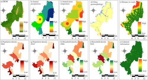
Urban wetlands are the target of many different elements of disturbance (Jiang et al. 2012) since they are susceptible to different climatic and human variables, which change depending on the geographic zone; we selected the driving factors based on a literature review, local expert knowledge, and data availability (Shaohui and Zhongping 2013; Tian et al. 2021). Table 1 presents the spatial datasets used for this study, including historical land use patterns, terrain conditions (elevation, geomorphology), positional data (distance to road network), climatic factors (temperature and precipitation), population and household density, and cadastral information.

Table 1. Data resources.

Data	Year	Type	Original resolution	Data resource
Images	1998, 2004, 2010	WMS resource	0.46 m	https://www.ideca.gov.co/recursos
Distance to the arterial road network		Vector	1:1000
DEM	2014	Raster	5 m
Urban geomorphology	2016	Vector	1:1000
Restricted Areas		Vector	1:1000
Population	2004, 2010	Document	Administrative	http://www.bogota.gov.co/
Cadastral information	1998, 2004, 2010	Vector	1:1000	https://serviciosgis.catastrobogota.gov.co/
Annual Mean Temperature		Vector	1:1500	https://datosabiertos.bogota.gov.co/
Annual Precipitation		Vector	1:1500
Annual Mean Precipitation		Vector	1:1500

The rasterized land-use maps were derived from the interpretation of three satellite images, one analog, and two numerical, corresponding to 1998, 2004, and 2010. Table 2 shows the area of each land use class for each year.

Table 2. Area (ha) of each land use class.

Land use class	1998	2004	2010
Constructions	21 849.4	22 544.7	22 995.3
Crops and pastures	6 709.9	5 996.9	5 499.3
Quarries	254.1	243.9	244.3
Urban Green Spaces	1 592.1	1 659.5	1 758.7
Water	136.8	136.8	137.9
Wetlands	810.2	770.7	717.0

The distance to the arterial road network was calculated using the ArcGIS Euclidean distance tool (ESRI 2020). The restricted areas data are the protected zones established in the city’s Land Use Plan (Secretaria Distrital de Ambiente, 2019). All the spatial datasets were rasterized, resampled to the same spatial resolutions of 5 and 30 meters (Figure 2), and normalized to eliminate quantitative and dimensional differences.

Figure 1. Study area of Bogota, Colombia.

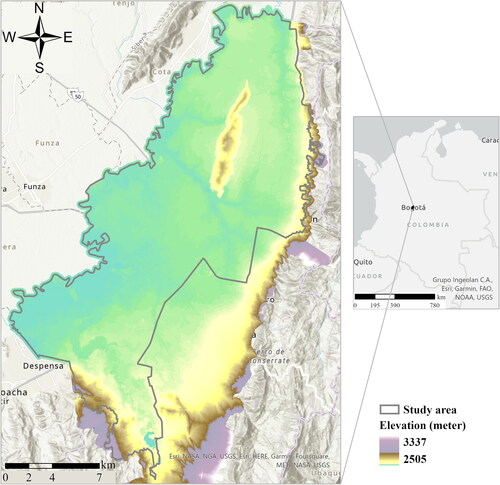
Figure 2. Driving factors - a detailed map of urban geomorphology together with the legend is attached as Appendix (see Figure A.1).

2.2. Methodology

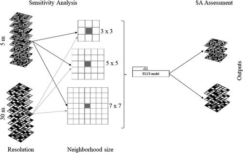
The methodology to perform the SA and its assessment consist of two steps, which are presented in Figure 3. The first step is simulating future land use changes using the FLUS model and carrying out the SA by varying the spatial resolution of the dataset from 5 to 30 meters and the neighborhood size between 3 × 3, 5 × 5, and 7 × 7. The second step is assessing the SA results using different qualitative and quantitative methods such as cross-classification maps, FoM, PA, OA, quantity and allocation disagreement, cross-classification maps, different landscape metrics, the TOC, and the fuzzy index.

Figure 3. Schematic diagram of the methodology.

2.2.1. FLUS model

The FLUS model has been applied successfully in other studies of urban dynamics (Liang et al. 2018; Zhang et al. 2021). Its implementation of a proportionate fitness selection gives the model a higher precision for obtaining consistent results compared to the reference data. It simulates land-use change under human and natural pressure using a spatial simulation process based on a CA model. Firstly, it uses an artificial neural network (ANN) to obtain the appropriate probabilities of the land-use classes from historical land-use data and the driving factors. The rules for the CA are drawn from those probabilities of occurrence. Then, its adaptive inertia and competition mechanisms allow the model to process the complex land-use interactions and competition locally, which can deal with the uncertainty and complexity of the change between the land-use classes under the effect of the driving factors (Liu et al. 2017).

Additionally, the FLUS model uses the Moore neighborhood to represent the neighborhood space. A total of 6 simulations were made to analyze the effects of neighborhood size and spatial resolution on the FLUS model results. The FLUS model has a Markov Chain module in which users can forecast future land-use demands by determining the transition probability of change from one category to another in a time interval. Nevertheless, we use the observed changes during the study period to feed the model and obtain the six outputs with different initial configurations.

Comprising the ANN of three-layer types: an input layer, a hidden layer, and an output layer, in the FLUS model, each neuron in the input layer corresponds to an input variable, land-use data, and driving variables. Likewise, each neuron in the output layer corresponds to a specific land-use type. Table 1 shows the variables selected as the influencing factors. For a detailed description of the FLUS model, see Liu et al. (2017).

2.2.2. Sensitivity analysis

A SA aims to understand how the variation in the model output can be apportioned to different sources of model parameter variations and how the given model depends upon the information fed into it (Crosetto et al. 2000). SA is a required step of modeling practice because it determines the model credence and aid in assessing uncertainties in the model results (Kocabas and Dragicevic 2006). Many techniques for SA have been proposed, including linear regression, measures of importance, Monte Carlo analysis, and correlation measures (Crosetto et al. 2000). There are two types of SA techniques. On the one hand, the univariate SA examines the model result concerning the variation of only one parameter at a time while the other parameters remain constant. On the other hand, the multivariate SA systematically varies multiple input parameters and determines the impacts on the analyzed outcome (Kocabas and Dragicevic 2006).

Further, SA can also be a tool for pre-calibration analysis (Crosetto et al. 2000). Generic procedures to perform SA on spatial models have been done. For example, Crooks et al. (2008) investigated the influence of the size of neighborhoods and the influence of geographical features in a residential segregation model tuned to London data. The analysis showed that the geometry of an area could act as a physical barrier to segregation. Shafizadeh-Moghadam et al. (2017) evaluated the effects of CA with different neighborhood sizes on the predictive performance of a Land Transformation Model.

Similarly, Wang et al. 2021 examined the effects of cell size on the performance of the transition rules of a CA model. SA techniques are usually applied to produce simulated outcomes that imitate the patterns observed in the real world. However, the sensitivity procedure in this paper explores the influence of two input parameters, i.e. neighborhood size and spatial resolution, on the model output. We run six simulations using three different neighborhood sizes in combination with 5 m and 30 m spatial resolutions.

2.2.3. Sensitivity Analysis assessment approach

Assessing the outcomes of a SA is crucial in spatial modeling applications (Kocabas and Dragicevic 2006). As such, this study aimed to evaluate the CA-FLUS model performance by undertaking a SA and a series accuracy assessment approach to understand the model’s sensibility to the variation of different parameters. We used many metrics suggested in the literature for a consistent SA evaluation. The assessment conception for the study uses univariate Sensitivity Analysis in which input factors are assumed independent. The presented SA assessment approach put together the qualitative and quantitative methods of cross-classification map, different landscape metrics, FoM, PA, OA, the AUC of the TOC curves, the Fuzzy Kappa index, and the disagreement metrics. The SA was achieved by varying the neighborhood size and the spatial resolution of the model inputs. We compared the model outcomes with real land-use data using different metrics. Table 3 provides descriptions of these metrics.

Table 3. Metrics used for SA assessment.

Approaches	Formula	Description
Figure of merit (FoM)	$\mathit{FoM}= \frac{B}{A+B+C+D}$	The FoM is the intersection of observed and simulated changes divided by the addition of observed and predicted changes^(a).
Producer accuracy (PA)	$PA= \frac{n_{ii}}{n_{+k}}$	PA indicates the proportion of pixels that the model simulates well as change^(a).
Overall accuracy (OA)	$OA={\sum }_{i=1}^k \frac{n_{ii}}{n}$	OA provides the general agreement between the reference map and the simulated one^(a).
Area under the curve for the Total operating characteristic (TOC)	$\mathit{AUC}={\int }_0^1\mathit{TPR} d(\mathit{FPR})$	TOC metric indicates how well the model is forecasting change^(b).
Fuzzy Kappa statistic	$K=\frac{P-E}{1-E}$	It is used to demonstrate the overall agreement between what is observed and what is simulated^(c).
Quantity disagreement (QD)	$Q=\frac{{\sum }_{g=1}^J{q}_g}{2}$	Measures the disagreement between the number of cells in each category without considering the spatial location^(d).
Allocation disagreement (AD)	$A=\frac{{\sum }_{g=1}^J{a}_g}{2}$	Evaluates the amount of disagreement between the reference map and the simulation map regarding the spatial location of the cells in each category^(d).

^a (Varga et al. 2019).

^b (Azari et al. 2022).

^c (Hagen-Zanker 2009).

^d (Pontius and Millones 2011a).

For the visual comparison of the CA model outcomes, we used the cross-classification maps. First, we assessed the categorical data errors with the confusion matrix by comparing outcome maps with the reference land-use maps (Crosetto et al. 2000). Within a confusion matrix, the true positives-true negative represents the correct number of pixels simulated, and the false positives-false negatives represent the errors of the simulated maps. The FoM is a well-known metric used for model validation via three-map comparison: reference beginning of the validation interval, simulation, and reference at the end of the validation interval (Varga et al. 2019). It goes from zero to one, meaning zero is no intersection between simulation and reference change, while one means perfect intersection between simulation and reference change. In Table 3, A is the proportion of error cells due to the observed change – predicted as persistence, B is the proportion of correct cells due to observed change – predicted as change, C is the proportion of error cells due to observed change modelling – predicted as a wrong gaining category, D is the proportion of error cells due to observed persistence – predicted as change and E denotes the area of correct cells due to observed persistence – predicted as persistence (Pontius et al. 2008).

The TOC is another analysis to evaluate the performance of land use models (Pontius and Si 2014). It is used to analyze the agreement between the output of a model with the reference map. The TOC shows misses, hits, false alarms, and correct rejections. As in the Receiving operating curve (ROC), the AUC of the TOC offers a metric to summarise the performance. The AUC has values on a scale from 0 to 1, where values between 0.90-1 means excellent, 0.80-0.90 indicates good, 0.70-0.8 signifies fair, and 0.60-0.70 poor accuracy level (Saha et al. 2021). In Table 3, TPR is the true positive rate or sensitivity that measures the fraction of the initial positives pixels which have been predicted correctly, and FPR is the false positive rate that indicates the fraction of the negatives pixels that have been selected as positive incorrectly (Fawcett 2006). A more detailed explanation of the TOC curve, used in land-change modeling, can be found in (Pontius and Si 2014).

The Fuzzy Kappa statistic agrees with two categorical raster maps (Hagen-Zanker 2009). It considers transition/change (Xu et al. 2019). Its values range from zero to one, where zero indicates no similarity and one identical similarity between the two maps. For the Fuzzy Kappa statistic in Table 3, P is the mean agreement, and E is the expected agreement. Additionally, another two measures proposed by Pontius and Millones (2011a) were applied: Quantity Disagreement (QD) and Allocation Disagreement (AD). Those indices are calculated through a contingency table for categorical variables, and their values vary from zero to one, where zero shows perfect agreement, and one indicates perfect disagreement. In Table 3, ${\sum }_{=1}^J{q}_g$ is the summatory of the global quantity disagreements of g classes in the reference and comparison maps. Similarly, ${\sum }_{g=1}^J{a}_g$ computes the allocation disagreement for all categories g is the summatory of the overall quantity disagreements of g categories in both reference and comparison maps. Similar to AD, ${\sum }_{g=1}^J{a}_g$ computes the allocation disagreement for all categories g (Pontius and Millones 2011b).

We calculated different landscape metrics to compare the structure and pattern of land-use classes simulated by the FLUS model. Landscape metrics are regarded as essential ecological planning tools and can aid urban land planners and managers in measuring the arrangement of landscape elements in time and space (Li et al. 2010). Therefore, the landscape metrics were calculated and examined across class (each patch type in the given mosaic) and at a landscape level (the landscape mosaic all considered together).

Class metrics calculate the aggregate properties of the patches that belong to a single class. Total area (CA) is an indicator of landscape composition that reveals how much of the landscape is comprised of a particular patch type (McGarigal and Marks 1994). The largest patch index (LPI) quantifies the rate of the total landscape area defined by the largest patch. The mean patch area (MN) is the sum across all patches of the corresponding patch type divided by the number of patches of the same class. Perimeter-area fractal dimension (PAFRAC) cast shape complexity across various spatial scales. A number of patches (NP) of a particular patch type are the total number of fragmented patches that belong to a specific land-use class. The aggregation index (AI) expresses the global agglomeration of the landscape. The total edge (TE) is the total length of the patch class. Area-Weighted Mean Shape Index (SHAPE_AM) weights patches conformable to their size. The landscape metrics also measure the aggregate properties of the complete patch mosaic (McGarigal and Marks 1994). The patch cohesion index (COHESION) measures the connectivity physical of each patch type. Contagion (CONTAG) measures patch-type combinations of units of different patch types and the spatial distribution of a patch type.

2.2.4. Software tools

The FLUS modeling tool was downloaded from https://www.geosimulation.cn/FLUS.html. Different tools were used to implement all the assessment techniques to evaluate the SA results. The OA was directly calculated from the FLUS model. The FoM and the PA were calculated from the confusion matrices. The cross-classification maps, quantity, and allocation disagreement were all run using TerrSet (Eastman 2020). The fuzzy kappa index was calculated with the Map Comparison Kit (MCK) (Visser and Nijs 2006). The AUC for the TOC curve was calculated using packages “raster” (Hijmans 2022) and “TOC” (Pontius and Si 2014) of the statistical software R (R Core Team 2020). Finally, the landscape metrics were computed in FRAGSTATS 4.2 (McGarigal and Marks 1994), and maps were produced with ArcGIS Pro 2.3 (ESRI 2020).

3. Results

The FLUS model was run to simulate 6-year land-cover changes in the case of urban wetland changes in Bogota, initiated in 2004 ($T_0$). The simulation time frame was selected to validate the results against the available land-use map corresponding to 2010. As a result, six simulation maps were generated with the wetland class as the target land use of the study. These correspond to a small area to the total space of the study area. Therefore, to correctly evaluate the SA outputs, we emphasized the wetlands cover assessment. This section presents the results obtained by varying the neighborhood size at different spatial resolutions and analyzing the results using the SA assessment approach.

Figures 4 and 5 illustrate the outcomes of cross-classification maps for 5 m and 30 m resolution. The first two rows present the resulting maps for neighborhood sizes 3 × 3, 5 × 5, and 7 × 7 of different areas of the study zone. The third row presents the cross-classification maps obtained to compare the simulations produced for the following combinations of neighborhood sizes: 3 × 3 vs. 5 × 5, 3 × 3 vs. 7 × 7, and 5 × 5 vs. 7 × 7.

Figure 4. Results from the SA assessment through cross-map method for 5 m spatial resolution. C (constructions), CP (crops and pastures), W (water), UGS (urban green spaces), Wet (wetlands).

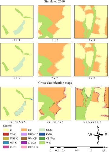
Figure 5. Results from the SA assessment through the cross-map method for 30 m spatial resolution. C (constructions), CP (crops and pastures), W (water), UGS (urban green spaces), Wet (wetlands).

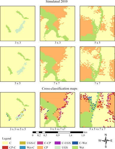
With the decrease of spatial resolution, the differences between the results from different neighborhood sizes become visually apparent for neighborhood size. However, as the difference between the neighborhood sizes is small, we need to establish which configuration is the best based on the visual evaluation. Then, this one was funded by the overall accuracy values (Table 4) of the cross-classification maps.

Table 4. Overall accuracy for cross-classification maps with wetlands mask.

Spatial resolution	Reference-Neighborhood size	Overall accuracy	Spatial resolution	Reference-Neighborhood size	Overall accuracy
5 m	3 x 3 vs 5 x 5	0.9893	30 m	3 x 3 vs 5 x 5	0.9701
	3 x 3 vs 7 x 7	0.9874		3 x 3 vs 7 x 7	0.9661
	5 x 5 vs 7 x 7	0.9871		5 x 5 vs 7 x 7	0.9639

The assessment results employing landscape metrics show that the FLUS model outcomes are sensitive to the changes in neighborhood sizes for different spatial resolutions.

Table 5 summarizes the class metrics results for all neighborhood sizes in 5 m and 30 m spatial resolutions. In addition, we calculated two more landscape metrics, the Patch cohesion index (COHESION) and Contagion (CONTAG). The COHESION value for the reference map (5 m) and the simulated map with a 3 × 3 neighborhood size were 99.95. Similarly, the COHESION value was 99.69 and 99.68 for the reference map and 5 × 5 neighborhood size simulation map with 30 m spatial resolution, respectively. CONTAG value for 5 m spatial resolution was 75.4 for the reference map and 74.23 for the 7 × 7 neighborhood size. For 30 m spatial resolution, the COHESION value for the reference map was 71.98 and 71.45 for 3 × 3 neighborhood size.

Table 5. Landscape metrics for neighborhood sizes 3 x 3, 5 x 5, 7 x 7 for 5 m and 30 m spatial resolution.

Neighborhood size	NP	LPI (%)	TE (m)	MN (m^2)	SHAPE_AM	PAFRAC	AI (%)
5 m
Wetlands
Reference	27	0.66	117 311.533	26.54	3.18	1.45	98.02
3 × 3	121	0.63	137 602.474	6.04	3.36	1.24	97.71
5 × 5	334	0.63	160 272.939	2.19	3.74	1.27	97.32
7 × 7	470	0.63	180 588.875	1.55	4.04	1.31	96.97
30m
Wetlands
Reference	29	0.66	109 020	24.71	3.08	1.38	88.84
3 × 3	40	0.63	115 350	18.28	3.29	1.38	88.28
5 × 5	42	0.63	118 830	17.41	3.36	1.39	87.92
7 × 7	54	0.63	123 900	13.54	3.44	1.40	87.40

Table 6 shows the results for the OA, PA, and FoM. Values of disagreement and agreement for the wetland land use class are presented in Table A1. For clarity in our results, the confusion matrices are in the Appendix from Tables A2 to A7.

Table 6. SA assessment of the outcomes indicated by the OA, PA, and FoM.

Neighborhood size 5 m spatial resolution	PA**	OA*	FoM**	Neighborhood size 30 m spatial resolution	PA**	OA*	FoM**
3 × 3	0.864104	0.9401	0.1082	3 × 3	0.8714	0.935115	0.1173
5 × 5	0.864104	0.9401	0.1107	5 × 5	0.86	0.934225	0.1267
7 × 7	0.864101	0.9398	0.1132	7 × 7	0.8608	0.931885	0.1363

* for the whole map.

** for the wetland land use class.

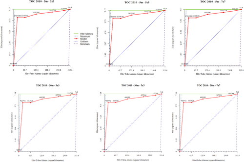
The AUC wetland values were estimated according to the TOC curves. In the Appendix, Figure A2 shows the TOC curves. Figure 6 depicts Figure A2 in detail, showing the first eight thresholds.

Figure 6. AUC of the TOC - zoom of Figure A.1 with thresholds.

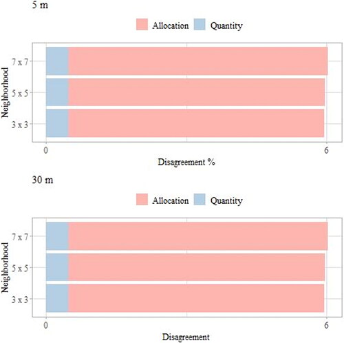
Fuzzy Kappa values showed an agreement between the simulation maps and the reference map between 0.41 and 0.90. For the wetlands category, the Fuzzy Kappa presented an agreement of 0.904 in 7 × 7 neighborhood size for 30 m spatial resolution. Assessment outcomes applying Fuzzy Kappa are shown in Figure 7. Another essential assessment approach was calculated bias QD and AD. Figure 8 shows the two components of disagreement for the three neighborhood sizes at 5 m and 30 m spatial resolution to the general extent. The two components of disagreement are piled to display how they amount to total disagreement. Specifically, the outcomes in 3 × 3 neighborhood size have 5.47% and 5.80% total disagreement for both spatial resolutions 5 m and 30 m, respectively.

Figure 7. Graph of fuzzy Kappa index and similarity above each bar for wetlands land-cover.

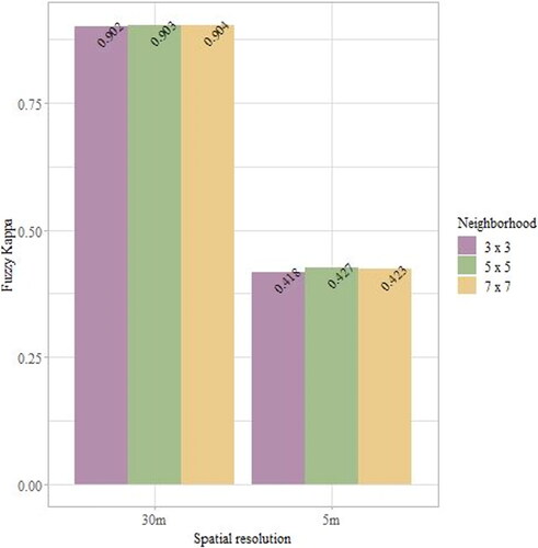
Figure 8. Quantity disagreement, allocation disagreement.

4. Discussion

We proposed a systematic application of a wide of quantitative and qualitative techniques in evaluating CA response to the variation of its parameters. The results of SA reveal interesting information about the model’s performance. First, the cross-maps depict areas where there are spatial differences. By increasing the size of the neighborhood, for both 5 m and 30 m spatial resolution, the contrast between the outcomes tends to be more evident visually. Then, cross-tabulation maps show spatial differences in model results when spatial resolution decreases. The overall accuracy values for the cross-classification maps (Table 4) decrease not only with the increase in neighborhood sizes but also with the increment of the spatial resolution. Nevertheless, the low differences between those values suggest that using different neighborhood sizes can result in similar simulation outcomes. In other words, cross-tabulation results comparing the neighborhood sizes at all spatial resolutions suggest moderate agreement.

Also, when the landscape metrics values are compared, the outcomes evidence that model results produce different landscape metrics. For example, the MN values decrease with increasing neighborhood size but increase with decreasing spatial resolution. By contrast, the PAFRAC, NP, TE, and SHAPE_AM values increase with increasing neighborhood size. For example, for the wetlands, land-use MN decreases from 6.04 to 1.55 for 5 m spatial resolution, and 30 m decreased from 18.28 to 13.54. Conversely, NP increased from 121 to 470 for 5 m.

Moreover, the model also seems sensitive to spatial resolution changes. NP and TE values decrease when the spatial resolution decrease. As a result, the land-use patterns are affected by changes in spatial resolution. Notably, for wetlands, land-use NP decreases from 121 to 40 with small neighborhoods from 5 m to 30 m spatial resolution, and TE values decrease from 137602.47 m to 115350 m. However, the largest patch index values present little variations for different neighborhood sizes and spatial resolutions.

In the same way, the aggregation index values do not vary a lot between the neighborhood sizes, but it decreases when decreasing spatial resolution. COHESION and CONTAG values hint that outcome maps are similar to the reference maps, having a closer similarity when using a 3 × 3 neighborhood size with 5 m spatial resolution.

Furthermore, the landscape metrics shown in Table 5 expose that outcome in a 3 × 3 neighborhood size with 30 m spatial resolution simulate better the target class (wetlands). Roodposhti et al. (2020) obtained similar results, suggesting that neighborhood rules are more important than neighborhood size when comparing different settings and analyzing the results with landscape metrics.

The OA, PA, and FoM indicators revealed that the model could perform well with varying neighborhood sizes. The model simulated at least 86% of the observed changed cells for 5 m resolution and over 94% of the unchanged cells. For the 30 m resolution combination, around 87% of the observed changed cells were correctly predicted, and over 93% of the unchanged cell. Despite at 30 m resolution combination having better accuracy results, the accuracy gain seems minor. Table 6 shows that FoM values change a lot between the resolutions. Although the FoM values are not highly accurate, they are acceptable because of the observed net change. R. Pontius et al. (2008) found a positive relationship between the FoM and the observed net change. As in this study, the simulation period is short (2004-2010), then the FoM values for the target category are accepted. The application of the previous metrics in the process of sensitivity evaluation of the CA showed similar accuracy outcomes when varying the neighborhood sizes as in the research of Shafizadeh-Moghadam et al. (2017), where the different neighborhood sizes (3 × 3, 5 × 5, 7 × 7, 9 × 9) produced somewhat similar results, although the 7 × 7 neighborhood size had a better performance.

Analysing the TOC curves, we notice that the configuration model of 30 m resolution with 3 × 3 neighbourhood size has the highest AUC, indicating a better performance than the other model configurations. For all simulations, TOC curves clasp the left side of the parallelogram because the wetlands in the reference map exist at the first-ranked values of each index in the output maps. In addition, the TOC curves for the indices touch the top bound of the parallelogram because some of the wetland’s absences are at the latter-ranked values. The thresholds shown in Figure 6 depict that the most significant number of hits derives from the simulation with 5 m resolution with a 7 × 7 neighbourhood. As the AUC of the TOC quantifies the relationship of the thresholds in general, we found that the AUC values were more significant than 0.95. Such good results indicate that the model performs well in the wetlands. Furthermore, AUC values increase when the neighborhood size and spatial resolution increase.

Figure 7 shows that the model can simulate well the land-use classes. Even though, of these outcomes, the 5 m spatial resolution simulated maps have the lowest Fuzzy Kappa values. By contrast, the wetlands category presented a high agreement in 7 × 7 neighborhood size for 30 m spatial resolution. The model is, therefore, sensitive to changes in spatial resolution. In addition, the quantity disagreement represents less than 6% of the global disagreement for both resolutions. Despite AD values being larger than QD, we consider these values acceptable because future research aims to obtain the probability of the net quantity of wetland changes.

Applying a wide range of techniques in assessing SA helped us better understand how the FLUS model responds to the resolution and neighborhood variations. However, the 3 × 3 neighborhood size with a 5 m spatial resolution model was more realistic than the other neighborhood sizes, and spatial resolutions were applied. Previous studies obtained similar results (Kocabas and Dragicevic 2006; Díaz-Pacheco et al. 2018; Roodposhti et al. 2020). CA models have been used to study LUCC to explore their complex dynamics at different spatial and temporal scales. Since this approach allowed us to represent the spatial complexity and its dynamics by choosing different configurations of its essential elements, such as the neighborhood size and spatial resolution, its implementation may help to minimize model errors and uncertainties, helping the modeler to find optimal combinations of its components, understanding how these variations influence the CA outcomes which will help to make better decisions in the land use management and urban planning process.

5. Conclusions

In this study, taking the land-use change process of Bogota from 1998 to 2010 as an example, we explored different assessment approaches for evaluating SA in the CA-FLUS model. A systematic method to assess SA in CA models was shown to represent real-world patterns as accurate as possible. SA validation was accomplished through the comparison of multiple quantitative and qualitative metrics. Calculating metrics such as the QD and AD helped us choose which path to take to improve the model’s prediction. Moreover, the landscape metrics applied allowed us to successfully determine the initial parameters configuration of the model, in order to better simulate the connectivity and patchiness of the wetlands. Despite the results demonstrating that the CA model outcomes are sensitive to neighborhood size and spatial resolution changes, all the initial configurations are generally acceptable to reproduce the land use change patterns in the study area. Strengths of this study include applying a wide range of evaluation metrics that help to better parameterize the model based on the objective of the model. Similarly, we were able to show that TOC, disagreement measures, and landscape metrics are sufficient to thoroughly evaluate the model performance since they reveal behaviors that quantitative measures such as FoM or PA and OA do not.

Concerning the limitations of this study, it is important to underline that they mainly come from the nature of the input data. For example, the data pre-processing step, such as the transformation from vector-to-raster and raster resampling, could have influenced the simulation outcomes; Díaz-Pacheco et al. (2018) have explored this type of limitation in further detail. It is also suggested to adopt other recent analyses proposed in the literature, such as the Intensity Analysis (Varga et al. 2019), which allow the assessment of the transition matrices. It considers the intensity of each category’s gross loss and gross gain concerning the temporal change overall. For future studies, we suggest the adoption of multiple approaches instead of just one or two to evaluate a model sensitivity and assess a model calibration. Methodological studies like this can facilitate the implementation of CA models by improving their calibration, goodness-of-fit and the validation stages.

Disclosure statement

No potential conflict of interest was reported by the authors.

Additional information

Funding

This work was supported by the Natural Sciences and Engineering Research Council (NSERC) of Canada through the Discovery Grant No RGP IN/05396–2016 awarded to Liliana Perez. Yenny Cuellar received financial support from the Department of Geography and Postgraduate and Postdoctoral Studies of the Université de Montréal; the Ministère de l’Enseignement supérieur du Québec; the Fondation Olivier Yvonne Poirier; and the Banque Nationale.

Appendix

Figure A1. Urban geomorphology.

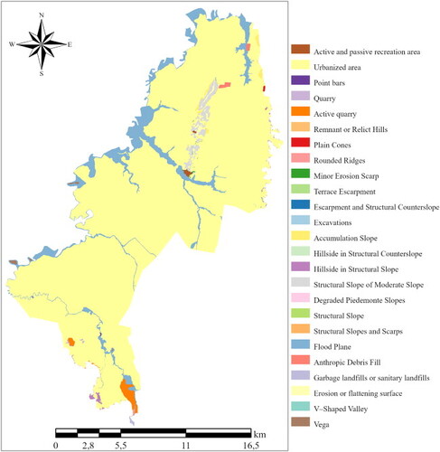
Figure A2. Sensitivity analysis using TOC for wetlands land use class.

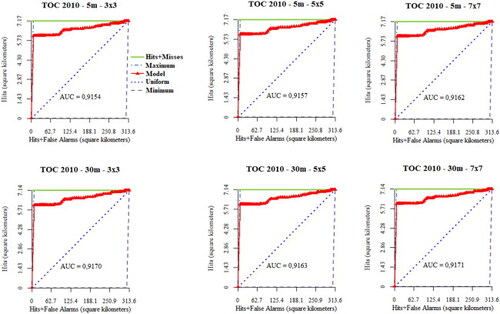
Table A1. Agreement and disagreement values for wetland land use class.

Resolution	Neighborhood	Change simulated as persistence	Correctly simulated change	Incorrectly simulated change	Persistence simulated incorrectly	Persistence simulated correctly
5 m	3 x 3	0.0035294605	0.0005201335	0.0001016665	6.562470e-04	0.01977552
	5 x 5	0.0035199717	0.0005315361	9.975273e-05	6.502666e-04	0.01978150
	7 x 7	0.0035100841	0.0005429387	0.0000982377	6.435686e-04	0.01978820
30 m	3 x 3	3.465304e-03	0.0005598461	0.0001090982	6.373633e-04	0.01983578
	5 x 5	3.419368e-03	0.0006000402	0.0001148402	6.029112e-04	0.01987023
	7 x 7	3.373432e-03	0.0006431053	0.0001177112	5.856852e-04	0.01988746

Table A2. Confusion matrix-5 m resolution 3x neighborhood size.

	C	CP	Q	UGS	W	Wet
C	1781037	52939	367	13055	8	3501
CP	43684	377758	0	7023	41	3916
Q	2	0	19226	0	0	0
UGS	12777	3617	0	119491	3	396
W	1	14	0	0	10856	12
Wet	2363	5999	0	286	74	49756

Table A3. Confusion matrix-5m resolution 5x neighborhood size.

	C	CP	Q	UGS	W	Wet
C	1781037	52939	367	13055	8	3501
CP	43684	377758	0	7023	41	3916
Q	2	0	19226	0	0	0
UGS	12777	3617	0	119491	3	396
W	1	14	0	0	10856	12
Wet	2363	5999	0	286	74	49756

Table A4. Confusion matrix-5m resolution 7x neighborhood size.

	C	CP	Q	UGS	W	Wet
C	1780874	52578	317	13459	8	3401
CP	43801	377024	0	6985	38	3966
Q	7	0	19223	0	0	0
UGS	12610	4260	0	119730	3	394
W	0	9	0	0	11133	9
Wet	2387	6211	0	309	61	49405

Table A5. Confusion matrix-30m resolution 3x neighborhood size.

	C	CP	Q	UGS	W	Wet
C	49304	1472	7	457	0	89
CP	1392	10300	0	196	1	106
Q	2	0	549	0	0	0
UGS	369	177	0	3292	0	11
W	0	0	0	0	300	0
Wet	72	163	0	5	1	1397

Table A6. Confusion matrix-30m resolution 5x neighborhood size.

	C	CP	Q	UGS	W	Wet
C	49387	1479	5	461	0	108
CP	1390	10362	0	206	0	112
Q	1	0	516	0	0	0
UGS	306	255	0	3099	0	11
W	0	0	0	0	297	0
Wet	63	173	0	11	1	1419

Table A7. Confusion matrix-30m resolution 7x neighborhood size.

	C	CP	Q	UGS	W	Wet
C	49235	1456	6	564	0	92
CP	1453	10349	0	185	0	116
Q	0	0	539	0	0	0
UGS	310	326	0	3141	0	8
W	0	0	0	0	317	0
Wet	54	168	0	6	1	1336

References

- Azari M, Billa L, Chan A. 2022. Multi-temporal analysis of past and future land cover change in the highly urbanized state of Selangor, Malaysia. Ecol Process [Internet]. 11(1):1–15. [accessed 2022 December 11].
- Crooks A, Castle C, Batty M. 2008. Key challenges in agent-based modelling for geo-spatial simulation. Comput Environ Urban Syst. 32(6):417–430. https://doi.org/10.1016/J.COMPENVURBSYS.2008.09.004
- Crosetto M, Tarantola S, Saltelli A. 2000. Sensitivity and uncertainty analysis in spatial modelling based on GIS. Agric Ecosyst Environ. 81(1):71–79.
- Díaz-Pacheco J, Delden H v, Hewitt R. 2018. The importance of scale in land use models: experiments in data conversion, data resampling, resolution and neighborhood extent. In: geomatic approaches for modeling land change scenarios lecture notes in geoinformation and cartography [Internet]. Cham: Springer; p. 163–186. [accessed 2022 February 19].
- Eastman JR. 2020. TerrSet 2020 Tutorial [Internet]. Clark University; p. 449. [email protected]
- ESRI. 2020. ArcGIS Pro. CA: Environmental Systems Research Institute.
- Fawcett T. 2006. An introduction to ROC analysis. Pattern Recognit Lett. 27(8):861–874.
- Feng Y, Gao C, Wang R, Li P, Xi M, Jin Y, Tong X. 2022. A moving window-based spatial assessment method for dynamic urban growth simulations. Geocarto International, 37-27, 15282-15301.
- Gaudreau J, Perez L, Drapeau P. 2016. BorealFireSim: a GIS-based cellular automata model of wildfires for the boreal forest of Quebec in a climate change paradigm. Ecol Inform [Internet]. 32:12–27.
- Hagen-Zanker A. 2009. An improved Fuzzy Kappa statistic that accounts for spatial autocorrelation. Int J Geograph Inform Sci [Internet]. 23(1):61–73. [accessed 2022 February 7].
- Hijmans RJ. 2022. raster: geographic data analysis and modeling. R package version 3.5-15; CRAN.
- Instituto Humboldt Colombia. 2018. Transiciones socioecológicas hacia la sostenibilidad. Gestión de la biodiversidad en los procesos de cambio en el territorio continental colombiano. Bogotá: Instituto Humboldt Colombia.
- Islam K, Rahman MF, Jashimuddin M. 2018. Modeling land use change using cellular automata and artificial neural network: the case of Chunati Wildlife Sanctuary, Bangladesh. Ecol Indic. 88:439–453.
- Jiang W, Wang W, Chen Y, Liu J, Tang H, Hou P, Yang Y. 2012. Quantifying driving forces of urban wetlands change in Beijing City. J Geograph Sci [Internet]. 22(2):301–314. [accessed 2022 May 30].
- Kantakumar LN, Kumar S, Schneider K. 2020. What drives urban growth in Pune? A logistic regression and relative importance analysis perspective. Sustain Cities Soc. 60(102269):102269.
- Kocabas V, Dragicevic S. 2006. Assessing cellular automata model behaviour using a sensitivity analysis approach. Comput Environ Urban Syst. 30(6):921–953.
- Li Y, Zhu X, Sun X, Wang F. 2010. Landscape effects of environmental impact on bay-area wetlands under rapid urban expansion and development policy: a case study of Lianyungang, China. Landsc Urban Plan [Internet]. 94(3–4):218–227.
- Liang X, Liu X, Li X, Chen Y, Tian H, Yao Y. 2018. Delineating multi-scenario urban growth boundaries with a CA-based FLUS model and morphological method. Landsc Urban Plan. 177:47–63.
- Liu X, Liang X, Li X, Xu X, Ou J, Chen Y, Li S, Wang S, Pei F. 2017. A future land use simulation model (FLUS) for simulating multiple land use scenarios by coupling human and natural effects. Landsc Urban Plan [Internet]. 168:94–116.
- McGarigal L, Marks BJ. 1994. FRAGSTATS manual: spatial pattern analysis program for quantifying landscape structure. [accessed 2022 February 7]. http://www.fs.fed.us/pnw/pubs/gtr_351.pdf.
- Misión Humedales de Bogotá. 2021. Misión para la gestión integral de los humedales Bogotá [Internet]. Secretaria de Ambiente. Bogota. https://ambientebogota.gov.co/documents/10184/2565901/Recomendaciones+POT.pdf/44c91c0e-0c08-4659-bfad-8d328aacf849.
- Pontius R, Boersma W, Jean-Christophe C, Keith C, De T, Nijs D, Charles D, Zengqiang F, Eric G, Noah K, et al. 2008. Comparing the input, output, and validation maps for several models of land change. Ann Reg Sci. 42(1):11–37.
- Pontius RG, Millones M. 2011a. Death to Kappa: birth of quantity disagreement and allocation disagreement for accuracy assessment Death to Kappa: birth of quantity disagreement and allocation disagreement for accuracy assessment. Int J Remote Sens [Internet]. 32(15):4407–4429. [accessed 2020 November 26].
- Pontius RG, Millones M. 2011b. Death to Kappa: birth of quantity disagreement and allocation disagreement for accuracy assessment. Int J Remote Sens. 32(15):4407–4429. [accessed 2020 November 23].
- Pontius RG, Si K. 2014. The total operating characteristic to measure diagnostic ability for multiple thresholds. Int J Geograph Inform Sci. 28(3):570–583.
- R Core Team. 2020. A language and environment for statistical computing. R Foundation for Statistical Computing. [Internet]. https://www.r-project.org/.
- Ramsar Convention Secretariat. 2019. La Colombie inscrit deux nouvelles Zones humides d’importance internationale [Internet]. https://www.ramsar.org/fr/news/la-colombie-inscrit-deux-nouvelles-zones-humides-dimportance-internationale.
- Roodposhti MS, Hewitt RJ, Bryan BA. 2020. Towards automatic calibration of neighbourhood influence in cellular automata land-use models. Comput Environ Urban Syst. 79(101416):101416.
- Saha TK, Pal S, Sarkar R. 2021. Prediction of wetland area and depth using linear regression model and artificial neural network based cellular automata. Ecol Inform [Internet]. 62:101272.
- Secretaria Distrital de Ambiente. 2019. Corredor Ecológico Ronda | Ideca [Internet]
- Shafizadeh-Moghadam H, Asghari A, Taleai M, Helbich M, Tayyebi A. 2017. Sensitivity analysis and accuracy assessment of the land transformation model using cellular automata. GIsci Remote Sens [Internet]. 54(5):639–656.
- Shaohui Y, Zhongping Z. 2013. Spatial-temporal changes of urban wetlands shape and driving force analysis using fractal dimension in Wuhan City, China. In: Proceedings of the 2013 International Conference on Remote Sensing, Environment and Transportation Engineering [Internet]. Paris, France: Atlantis Press; p. 540–543.
- Tian Y, Li J, Wang S, Ai B, Cai H, Wen Z. 2021. Spatio-temporal changes and driving force analysis of wetlands in Jiaozhou Bay. J Coast Res. 38(2):328–344.
- Tiné M, Perez L, Molowny-Horas R, Darveau M. 2019. Hybrid spatiotemporal simulation of future changes in open wetlands: a study of the Abitibi-Témiscamingue region, Québec, Canada. Int J Appl Earth Observ Geoinform. 74(September 2018):302–313.
- Tong X, Feng Y. 2019. A review of assessment methods for cellular automata models of land-use change and urban growth. Int J Geograph Inform Sci. 34(5):866–898. https://doi.org/10.1080/13658816.2019.1684499.
- Varga OG, Pontius RG, Singh SK, Szabó S. 2019. Intensity analysis and the figure of merit’s components for assessment of a cellular automata – Markov simulation model. Ecol Indic [Internet]. 101:933–942. [accessed 2021 December 20].
- Visser H, Nijs T. 2006. The map comparison next term kit. Environ Modell Software. 21(3):346–358.
- Wallentin G, Neuwirth C. 2017. Dynamic hybrid modelling: Switching between AB and SD designs of a predator-prey model. Ecol Modell. 345:165–175.
- Wang H, Guo J, Zhang B, Zeng H. 2021. Simulating urban land growth by incorporating historical information into a cellular automata model. Landsc Urban Plan [Internet]. 214(June):104168.
- Xu T, Gao J, Coco G. 2019. Simulation of urban expansion via integrating artificial neural network with Markov chain–cellular automata. Int J Geograph Inform Sci. 33(10):1960–1983. [accessed 2020 December 6]
- Zhang C, Wang P, Xiong P, Li C, Quan B. 2021. Spatial pattern simulation of land use based on flus model under ecological protection: A case study of hengyang city. Sustainability (Switzerland). 13(18):10458. https://doi.org/10.3390/su131810458.