Enhanced-resolution reconstruction for the China-France Oceanography Satellite scatterometer

Abstract

The China-France Oceanography Satellite SCATterometer (CSCAT) can observe radar backscatter values on the same sea surface at multiple incidence angles, and is often used to estimate the ocean near-surface wind. However, CSCAT utilizes a novel scanning mechanism and the wind vector cell has a spatial resolution is 25 km or 12.5 km, which limit the study of high-resolution land and sea ice monitoring. To address this issue, this paper constructs a geometric model of the main lobe-to-ground projection relationship and generates the enhanced-resolution radar images. CSCAT data are applied to three main image reconstruction algorithms (SIR, AART, and MART), and experiments are performed in the Iceland and Hudson Bay, and verified by Sentinel-2 optical remote sensing data. The experiments show the geometric model for CSCAT improves the spatial resolution from traditional 25 km to 5 km, and the SIR-reconstructed images are characterized by higher accuracy and better suppression of noise than are those obtained with the AART and MART methods. Therefore, this study extends the application of domestic remote sensors and provides data support for high-resolution applications, such as land and sea ice monitoring.

Keywords:

• China-France Oceanography Satellite
• scatterometer
• image reconstruction
• backscatter coefficient
• spatial response function

1. Introduction

The scatterometer is an active, nonimaging microwave radar sensor that can provide all-weather operation and is capable of achieving global coverage in a short time. By measuring the normalized radar cross section of the Earth’s surface, the scatterometer provides the basis for scientific research on near-surface wind vector inversion, vegetation, soil moisture inversion, and polar sea ice monitoring. The spaceborne microwave scatterometer currently in operation has the spatial resolution of 25–50 km, which limits research involving high-resolution terrestrial processes and sea ice monitoring. Image reconstruction relies on the excellent temporal resolution of the scatterometer to compensate for the low spatial resolution of the original data, and is suitable for areas with stable surface backscatter coefficients and slow changes, such as land areas and glaciers.

Image reconstruction algorithms are widely used in many scientific fields, such as medicine, radar astronomy, industrial nondestructive testing, and geological exploration. Currently, there are two main methods used for image reconstruction: analytical reconstruction and algebraic reconstruction. In the analytical reconstruction method, incomplete projection data are interpolated, and inverse projection is used to obtain a reconstructed image (Zhu 1993). Algebraic reconstruction involves transforming an image reconstruction problem into a problem in which linear equations must be solved using iterative algorithms, including the additive algebraic reconstruction technique (AART), the multiplicative algebraic reconstruction technique (MART) and scatterometer image reconstruction (SIR) (Gordon 1971; Herman et al. 1973; Censor 1983; Long et al. 1993; Early and Long 2001; Yun and Dong 2015). The algebraic reconstruction can incorporate image prior knowledge to fully utilize the a priori information of the study object, reduce the discomfort of image reconstruction, and help improve the quality and clarity of the reconstructed images. These three algorithms have made important contributions to scatterometer image reconstruction and resolution improvement, and are widely used in land exploration, vegetation research and polar sea ice exploration. For microwave scatterometers, image reconstruction methods are currently used for fixed fan-beam scatterometers and pencil-beam rotary scanning scatterometers. For fixed fan-beam scatterometers, Long et al. (1994) proposed an incidence angle-based sea ice image reconstruction method to reconstruct sea ice scattering images at the higher resolution than that of the original data using 7 days of data from the ERS-1 scatterometer. Lindsley and Long (2016) applied an image reconstruction algorithm to L1B-level data from ASCAT and used 5 days of data to effectively improve the spatial resolution of the reconstructed images. For pencil-beam rotary scanning scatterometers, Remund and Long (2014) proposed an operational sea ice mapping algorithm based on SeaWinds data using image reconstruction methods. Yun and Dong (2015) performed a simulation study of high-resolution backscatter coefficient image reconstruction techniques using the HY-2 microwave scatterometer. Kunz and Long (2005) used images reconstructed from SeaWinds data to analyze the daily variations in sigma0 in the Sahara Desert. Spencer et al. (2000) demonstrated the utility of SeaWinds reconstructed images in studies of land and snow areas. Meier and Stroeve (2008) distinguished sea ice from seawater using the SIR method based on QuikSCAT data. Swan and Long (2012) extracted scattering histograms of sea ice types based on QuikSCAT scatterometer sea ice reconstruction images and dynamically adjusted sea ice classification thresholds. Long (2017) compared the SIR algorithm with ‘drop in the bucket’(DIB) and ‘fine-resolution DIB’(fDIB) algorithm based on SeaWinds data, demonstrating the effectiveness of high-resolution reconstruction using SIR as well as its limitations and the limitations of DIB and fDIB. Backscatter data from fixed fan-beam scatterometers and pencil-beam rotary scanning scatterometers have been combined with image reconstruction techniques and applied in many land and ice studies, but fixed fan-beam scatterometers have a blind scan swath, cover the global sea surface slowly, and require the use of multiple days of data for image reconstruction, which can lead to blurred observations of moving features. Additionally, the observation time of pencil-beam rotary scanning scatterometers is shorter for the same target. Still, fewer independent measurement samples can be obtained with this scatterometer, which affects the accuracy of the backscatter coefficient (Lang and Lin 2017), and thus the accuracy of scatterometer-based image reconstruction.

The China-France Oceanography Satellite (CFOSAT), launched in 2018, carries a SWIM which is used to monitor wave spectrum on the sea surface and a microwave scatterometer. CSCAT adopts a new mode of HH and VV dual-polarized fan-beam rotary scanning, combining the advantages of fixed fan-beam and pencil-beam rotary scanning scatterometers, with high overlap of observations of the Earth (including polar regions), a short revisit period, and multiangle observation capabilities; thus, the density of the ground footprint of CSCAT is more than 10 times higher than that of single-incidence-angle scatterometers, providing both high spatial resolution and high temporal resolution. Therefore, the multiangle observation capability of CFOSAT provides a good basis for land and sea ice monitoring studies. Recently, Lin et al. (2021) used CFOSAT to study coastal wind retrieval, but there have been few studies that have applied CSCAT data in image reconstruction. In this paper, we use the CSCAT antenna pattern to construct a geometric model of the main lobe-to-ground projection relationship of CSCAT to estimate a simplified spatial response function. Then, this function is used with CSCAT backscatter measurements to produce enhanced-resolution reconstructed backscatter images of land and seas using the SIR, AART, and MART algorithms. The resulting images improve the spatial resolution the traditional 25 km to 5 km. The three methods are compared to obtain the optimal image reconstruction algorithm for CSCAT. This study demonstrates the use of image reconstruction techniques for rotating fan-beam antenna scatterometers to produce finer resolution backscatter images to support applications such as land and sea ice monitoring.

2. Materials and methods

We use the CSCAT antenna pattern to construct a geometric model of the main lobe-to-ground projection relationship of CSCAT to estimate a simplified spatial response function. Then, this function is used with CSCAT backscatter measurements to produce enhanced-resolution reconstructed backscatter images of land and seas. In this section, we introduce the study area, CSCAT scanning mechanism, geometric model construction of the main lobe-to-ground projection relationship and microwave scatterometer image reconstruction method.

The geometric model of the main lobe-to-ground projection relationship is necessary to obtain the ground footprint morphology of the scatterometer for image reconstruction. Since the antenna configurations of microwave scatterometers with different scanning mechanisms are different, resulting in different observation geometries that directly affect the ground footprint morphology and effective beamwidth of observations and thus affect image reconstruction, it is necessary to construct a geometric model of the main lobe-to-ground projection relationship for CSCAT, a new scanning mechanism.

2.1. Study area

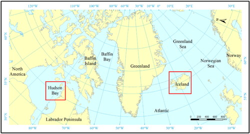
The study areas selected in this paper are Iceland and the Hudson Bay, and the two study areas have different scattering characteristics. Iceland is located in the middle of the North Atlantic and bordered by the Greenland Sea to the north, and inland by plains and glaciers. The first study area mainly consists land, and it is fixed and immobile. The second study area is Hudson Bay. The climate is cold, and ice and ice floes are present in the bay at all times except from August to September. The second study area is mainly sea ice except for a few islands, and it is mobile. The study areas are shown in Figure 1, and the red rectangular boxes are the image reconstruction areas.

Figure 1. The study areas.

Three days of data from January 22 to January 24, 2020, were selected, with data from 22 orbits. The CSCAT L1B data (v10.10) were obtained from the website of the National Satellite Ocean Application Service in Network Common Data Form (NetCDF). The latitude and longitude of the footprint center of each pulse, latitude and longitude of each slice center, slice center azimuth angle, slice center incidence angle, antenna elevation angle and backscatter coefficient were extracted from the NetCDF file. Since the signal-to-noise ratio of HH-polarized data is generally lower than that of VV-polarized data (Liu et al. 2020), resulting in larger σ⁰ measurement error in HH-polarized data, thus the VV-polarized data were selected for image reconstruction in this paper.

2.2. CSCAT scanning mechanism

CSCAT carries a scatterometer antenna that transmits pulsed signals to the Earth for 24 h at 3.4 revolution per minute (rpm) and at an incidence angle of 28°-51°; the swath is greater than 1000 km, and the scatterometer orbits the Earth 14-15 times a day (Lin 2011). CSCAT achieves 96.55% coverage of Earth in 3 days (Wang et al. 2019). Compared to other scatterometers, CSCAT has much higher temporal resolution. Figure 2(a) shows the observation schematic of the CSCAT, and Figure 2(b) shows the fan-beam footprint schematic.

Figure 2. (a) Observation schematic of the CSCAT, (b) Schematic of fan-beam footprint.

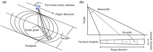
The rotary scanning mechanism of the fan-beam adopted by CSCAT can avoid subsatellite point gap issues and achieve fast coverage with a large swath; additionally, both elevation and azimuthal ground backscatter coefficients can be determined, which shortens the time required to obtain multiple azimuth observations in the same area. With the motion of the satellite, CSCAT can observe the same surface features at different azimuth and incidence angles several times during an orbit pass with the rotary scanning process, and obtain more observation angle measurements than previous spaceborne radar scatterometers (Zhu et al. 2013; Dong et al. 2020), especially in polar regions where the overlap of data is high. Thus, CSCAT is particularly suitable for the reconstruction of land and sea ice images in the polar regions.

CSCAT combines the features of fixed fan-beam and pencil-beam rotary scanning scatterometers. As shown in Figure 2(b), the working mode for CSCAT is rotational scanning, and CSCAT scans conically around the axis of the satellite nadir point. Since the flight attitude of the satellite is variable, the shape and range of different fan footprints of the scatterometer differ; therefore, establishing the relationship between the antenna and the footprint pattern is an important prerequisite for obtaining the optimal footprint pattern.

2.3. Geometric model construction of the main lobe-to-ground projection relationship

The antenna beam of the scatterometer emits microwave pulses to the Earth, and the antenna energy covers a certain portion of the Earth’s surface and it is distributed in the main lobe and sidelobe of the antenna. Although sidelobes also have information that can contribute to the reconstruction (Early and Long 2001), notably, the main energy from antenna radiation is concentrated in the beamwidth of the antenna main lobe, that is, the width between the two half-power points of the main lobe of the antenna pattern. Therefore, the information within the beamwidth of the antenna main lobe reflects the information associated with the target feature, and image reconstruction with scatterometer data is actually the reconstruction of the information within the beamwidth of the antenna main lobe. Note that the sidelobes is not considered in this paper.

1. Beamwidth of the antenna main lobe of the fan-beam rotary scanning scatterometer

For a rectangular antenna with a narrow beamwidth in the azimuth direction, a simple Cartesian coordinate system can be used to represent the main lobe pattern on the surface. The antenna pattern of the CSCAT transmitting VV-polarized beam is plotted according to the scanning angle and antenna gain in Figure 3, where the red line indicates the azimuth antenna pattern and the blue line indicates the elevation antenna pattern.

Figure 3. The pattern of the VV-polarized antenna.

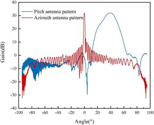
Figure 3 shows that the main lobe energy of the azimuth pattern of the VV-polarized antenna is concentrated at approximately 0°, and the amount of sidelobe information gradually decreases at other angles. Additionally, the main lobe energy of the elevation pattern of the VV-polarized antenna is concentrated at approximately 40°. According to the scatterometer antenna pattern of CSCAT, the beamwidths of the main lobe in the azimuth and elevation directions under VV polarization are $\begin{array}{c}{\beta }_{az}=1.2°\\ \end{array}$ and ${\beta }_{el}=14.5°,$ respectively.

2.	Geometric model of the main lobe-to-ground projection

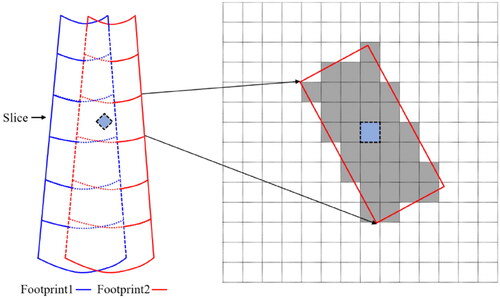
A range-compressed CSCAT pulse is divided into 40 scattering cells on the surface arranged along the beam footprint in the shape of a long fan as shown in Figure 2(b). Thus, the observed values obtained by CSCAT are the backscatter coefficients of the 40 scatter cells. From the observation geometry of CSCAT, the azimuth beamwidth is approximately 1.15°, and the length of the fan-beam footprint in the range direction is approximately 500 km; this footprint is divided into 40 parts, and the length of each slice in the range direction is approximately 12.5 km. Additionally, the original resolution of the fan footprint is 10.5 km, the parallel sides of each slice are approximately equal, and the slice geometry can be approximated as a rectangle. To obtain the coverage of the antenna main lobe beamwidth to ground footprint, the scatter points are reduced to the form of slices according to the geometric model of the main lobe-to-ground projection in this paper.

The unification of the reconstructed coordinate system and the coordinate system established in the flight direction is performed based on the center position of each slice, and the distances in the elevation and azimuth directions are calculated from the known center position of the slice and the beamwidths in the elevation and azimuth directions to obtain the size and position of the antenna main lobe beamwidth to ground footprint. Based on the conversion relationship (see Equation (1)(1) $$\left(\begin{array}{c}{x}_{\mathit{flight}}\\ y_{\mathit{flight}}\end{array}\right)=\left(\begin{array}{cc}\hspace{0.17em}\cos \hspace{0.17em}\theta & -\hspace{0.17em}\sin \hspace{0.17em}\theta \\ \hspace{0.17em}\sin \hspace{0.17em}\theta & \hspace{0.17em}\cos \hspace{0.17em}\theta \end{array}\right)\left(\begin{array}{c}{x}_{\mathit{recons}}\\ y_{\mathit{recons}}\end{array}\right)$$(1) ) between the coordinate system established in the flight direction and the reconstructed coordinate system, the footprint profile information is transferred to the reconstructed coordinate system. (1) $$\left(\begin{array}{c}{x}_{\mathit{flight}}\\ y_{\mathit{flight}}\end{array}\right)=\left(\begin{array}{cc}\hspace{0.17em}\cos \hspace{0.17em}\theta & -\hspace{0.17em}\sin \hspace{0.17em}\theta \\ \hspace{0.17em}\sin \hspace{0.17em}\theta & \hspace{0.17em}\cos \hspace{0.17em}\theta \end{array}\right)\left(\begin{array}{c}{x}_{\mathit{recons}}\\ y_{\mathit{recons}}\end{array}\right)$$(1) where $\hspace{0.17em}\cos \hspace{0.17em}\theta =\frac{x_{\mathit{recons}}-x_1}{\sqrt{{(x_{\mathit{recons}}-x_1)}^2+{(y_{\mathit{recons}}-y_1)}^2}},$ $\hspace{0.17em}\sin \hspace{0.17em}\theta =\frac{y_{\mathit{recons}}-y_1}{\sqrt{{(x_{\mathit{recons}}-x_1)}^2+{(y_{\mathit{recons}}-y_1)}^2}}$ is the rotation factor, $(x_{\mathit{recons}},y_{\mathit{recons}})$ is the coordinate of the slice center position in the reconstructed coordinate system, and $(x_1,y_1)$ is the coordinates of one pulse(cell).

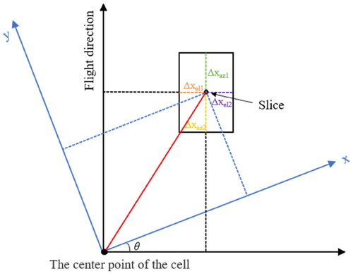
Figure 4 shows the geometry of the footprint slice calculated based on the corner point parameters. The rectangular box indicates the range of the antenna main lobe beamwidth to ground footprint, the black coordinate system is the coordinate system established in the flight direction, and the blue coordinate system is the coordinate system established for the image to be reconstructed.

Figure 4. The geometry of the footprint slice.

3.	Spatial response function

In general, it is assumed that the ground σ⁰ data is based on sampled data from a two-dimensional grid of the ground and the measurements are obtained by filtering the Spatial Response Function (SRF) on the received electromagnetic wave information. The SRF of the scatterometer represents the contribution of each image element in the two-dimensional grid divided by the antenna footprints to the actual observations, and SRF is used to describe the antenna gain distribution in the same two-dimensional grid as the ground at the time of sampling. Since the scatterometer is a non-imaging sensor, the ground σ⁰ distribution is equivalent to a two-dimensional grid image, and the SRF determined by the antenna pattern is equivalent to the filter operator.

In a scatterometer backscatter model (Liu et al. 2017), the SRF is required to realize high-resolution image reconstruction. The accuracy of the SRF influences the accuracy of the reconstructed image. The SRF is a combined effect of antenna gain pattern and radar ambiguity function, and the SRF varies with the antenna azimuth and orbital position; moreover, the conventional SRF is computationally intensive to obtain (Ashcraft and Long 2003). However, because the scatterometer slice response is concentrated in the main lobe, setting $h(x,y)$ inside the footprint to 1 and $h(x,y)$ outside the footprint to 0 can significantly reduce the number of computations and the computational complexity with only a small loss of image quality (Ashcraft and Long 2003; Gang et al. 2015). Therefore, in the paper we consider this loss is acceptable and the impact on the results can be ignored, and taking this as a prerequisite, a simplified SRF model is constructed for the sake of computational convenience and efficiency.

The scatterometer slice coverage is determined by corner points, the coordinates of the corner points are calculated based on geometric projection, and the overlapping image pixels are calculated for all slice coverages. The two footprints of CSCAT are shown schematically in the left image in Figure 5, and the right image corresponds to a slice covering the imaging grid in the left image; notably, the slice is pixelized based on the imaging grid. The black grid on the right is the pixel grid assigned to the unknown image, the thick red rectangular box is the ground coverage contour of a particular slice, and the gray grid indicates that the grid center is contained within the contour of the slice; at this point, $h(x,y)=1;$ otherwise, $h(x,y)=0$ In defining the gridded image, a pixel sampling of at least two pixels per slice width is required as a guarantee that the final obtained value is reasonable, which is also a constraint of the reconstructed image resolution (Long and Luke 2003). The nominal pixel size for reconstruction in this paper is 5 km to correspond to the minimum slice width of 10 km.

Figure 5. Pixelation of slice on the imaging grid.

2.4. Microwave scatterometer image reconstruction method

2.4.1. SIR algorithm

Image reconstruction techniques can improve the spatial resolution of existing remote sensing acquisitions to some extent by overlapping the ground coverage areas of adjacent independent measurements (Gang et al. 2015). Image reconstruction algorithms are based on overlapping multiple ground coverages. In SIR, an initial value is assigned to each pixel in the image, and these values are then iteratively updated with multiplicative updating to continuously best approximate the true values. The SIR algorithm is expressed as follows (Long et al. 1993): (2) $$p_j^{k+1}=\frac{1}{{\sum }_{i=1}^{N_m}{h}_{ij}}\sum _{i=1}^{N_m}{h}_{ij}{\left(u_{ij}\right)}^k$$(2) where $h_{ij}$ denotes the effective spatial response function for the i^th measurement corresponding to the j^th pixel, k is the number of iterations, the range of j is $\left[1,M\right],$ M is the number of pixels in the image, $p_j^{k+1}$ denotes the k + 1^th iteration of p for the j^th pixel, $N_m$ denotes the number of measurements, and the update term $u_{ij}$ is defined as follows: (3) $${\left(u_{ij}\right)}^k=\{\begin{array}{c}{\left[\frac{1}{2}\frac{1}{f_i^k}\left(1-\frac{1}{d_i^k}\right)+\frac{1}{p_j^k{d}_i^k}\right]}^{-1},d_i^k\ge 1\\ \left[\frac{1}{2}{f}_i^k\left(1-d_i^k\right)+p_j^k{d}_i^k\right],d_i^k<1\end{array}$$(3) where $f_i^k$ is the forward measurement projection, $d_i^k$ is the scaling factor, and $f_i^k$ and $d_i^k$ are, respectively: (4) $$f_i^k=\frac{1}{{\sum }_{j=1}^M{h}_{in}}\sum _{j=1}^M{h}_{in}{p}_n^k$$(4) (5) $$d_i^k={\left(\frac{z_i}{f_i^k}\right)}^{\raisebox{1ex}{$1$}\!\left/ \!\raisebox{-1ex}{$2$}\right.}$$(5)

The iterative process starts from the initial values in vector form, and the magnitude of the scale factor $d_i^k$ is determined. Then, the image is continuously corrected until the iteration is completed. Since the algorithm uses different update terms for different scale factors, the sensitivity to noise is reduced. In this paper, the initial values are obtained based on the inverse distance weighted (IDW) interpolation of measurements, which is an exact interpolation process (Liu et al. 2021). Notably, each interpolated surface passes through a sample point, ensuring that the interpolation result is consistent with the actual backscatter coefficient at the sample point. IDW interpolation is combined with the SIR algorithm to reconstruct images based on a uniformly sampled high-resolution grid using irregularly sampled data.

2.4.2. AART and MART algorithms

In the additive algebraic reconstruction technique, an initial value is assigned to each pixel in the image, and an additive update term is then used to iteratively update each value to continuously approximate the true value. The AART algorithm is expressed as follows (Early and Long 2001): (6) $$p_j^{k+1}=p_j^k+\frac{{\sum }_i\left(z_i-f_i\right)h_{ij}}{{\sum }_i{h}_{ij}}$$(6) where $p_j^k$ is the k^th valid estimate for pixel j. The iterative process starts from the initial value of the vector, and initial values are continuously corrected until the iteration is completed.

The multiplicative algebraic reconstruction technique is similar to the AART algorithm but iteratively updates the pixels with multiplicative updated terms. Specifically, the MART algorithm is expressed as follows (Yun and Dong 2015): (7) $$p_j^{k+1}=\frac{1}{{\sum }_{i=1}^{N_m}{h}_{ij}}\sum _{i=1}^{N_m}{h}_{ij}{(u_{ij})}^k$$(7) (8) $$u_{ij}^k=p_j^k{\left(\frac{z_i}{f_i^k}\right)}^{\raisebox{1ex}{$1$}\!\left/ \!\raisebox{-1ex}{$2$}\right.}$$(8)

The update term for each pixel is the current estimate multiplied by the ratio of the measurement to the forward estimate.

2.4.3. Incidence angle normalization

Over a limited incidence angle range, between 28° and 51° for the CSCAT, the incidence angle dependence of backscatter is approximately linear in dB. Although the actual incidence angle dependence of σ⁰ in dB is nonlinear, the linear model works very well for the mid-range incidence angles as observed in the actual and theoretical backscatter results (Drinkwater et al. 1994). The linear model is given by the equation. (9) $${\sigma }_{dB}^0=\mathcal{A}+\mathcal{B}(\theta -{40}^{\circ })$$(9) where ${\sigma }_{dB}^0$ is the received backscatter power in dB and θ is the incidence angle of the measurement. Note that the measurements are normalized to 40°, i.e. the actual measurement is adjusted to represent a measurement taken at 40°. Although 40° is used here, the data can be normalized to any incidence angle value. Thus $\mathcal{A}$ is the backscatter power from the surface at 40°, and $\mathcal{B}$ represents the slope, or dependence, of ${\sigma }_{dB}^0$ with respect to the incidence angle θ of the measurement. In the reconstruction, we will estimate the $\mathcal{A}$ from the data.

3. Results

3.1. Iceland

3.1.1. Comparison of the AART, MART and SIR algorithms

Image results from the three methods, AART, MART and SIR, are compared. Due to the noise in the measurements, increasing the number of algorithm iterations may improve the reconstruction accuracy, but high-frequency noise is amplified. To measure the reconstruction accuracy of the backscatter coefficients, the normalized standard deviation $K_p$ is introduced, as shown in Equation (10)(10) $$K_p=\frac{\sqrt{\mathrm{var}({\tilde{\sigma }}^0)}}{E({\tilde{\sigma }}^0)}$$(10) . (10) $$K_p=\frac{\sqrt{\mathrm{var}({\tilde{\sigma }}^0)}}{E({\tilde{\sigma }}^0)}$$(10) where $\mathrm{var}({\tilde{\sigma }}^0)$ is the ${\tilde{\sigma }}^0$ variance and $E({\tilde{\sigma }}^0)$ is the ${\tilde{\sigma }}^0$ mean. The two variables are approximated by the sample variance and sample mean of the reconstructed results. The smaller the normalized standard deviation is, the higher the reconstruction accuracy of the image is. $K_p$ is the average value of σ⁰ over the study area.

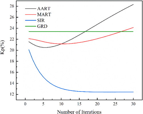
Either too early or too late termination of the iterative optimization algorithm can produce signal reconstruction bias, which can cause spatial blurring of the image or signal. A large number of iterations improves the reconstruction accuracy at the expense of increased noise. Thus, different iterations are needed for different algorithms to achieve the optimal image reconstruction accuracy under the current algorithm. Figure 6 shows the relationship between the normalized standard deviation and the number of iterations. Since the smaller the normalized standard deviation is, the higher the reconstruction accuracy of the image is, the number of iterations corresponding to the smallest normalized standard deviation is chosen as the final iteration number of the algorithm in this paper. In Figure 6, the normalized standard deviation of SIR decreases as the number of iterations increases, and the algorithm converges after 20 iterations. The $K_p$ value of the AART algorithm changes from decreasing to increasing rapidly after 6 iterations because the noise is further amplified with the number of iterations. Additionally, the $K_p$ value of the MART algorithm changes from decreasing to increasing after 10 iterations, but the rate of change slows and the overall trend is flat. The minimum $K_p$ values of the AART and MART algorithms are 20% and 21%, respectively, while the normalized standard deviation of the SIR algorithm is stable at 12% as the number of iterations increases, indicating that the reconstruction accuracy of the SIR algorithm is higher.

Figure 6. Normalized standard deviation of AART, MART and SIR as a function of the number of iterations for Iceland region.

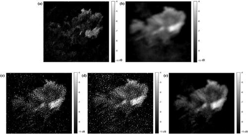
Figure 6 shows that the AART, MART, and SIR algorithms reconstruct the images with the highest accuracy after 6, 10, and 20 iterations, respectively. Figure 7 shows the reconstruction results of different algorithms for the Iceland region, where Figure 7(a) shows the original backscatter coefficient distribution, Figure 7(b) shows fDIB GRD image, Figure 7(c) shows the image reconstructed with the AART algorithm after 6 iterations, Figure 7(d) shows the image reconstructed with the MART algorithm after 10 iterations, and Figure 7(e) shows the image reconstructed with the SIR algorithm after 20 iterations. Notably, Figure 7 illustrates that all three enhancement algorithms can reconstruct the features of Iceland from CSCAT data, although there is considerable noise in the images reconstructed with the AART and MART algorithms. Additionally, the amount of high-frequency noise in the images reconstructed with the SIR algorithm is significantly reduced, which indicates that the SIR algorithm has better noise suppression ability than the other algorithms. The SIR-reconstructed image of Iceland is clear, and the dark part is the ocean, indicating that the land and the ocean can be clearly distinguished. Moreover, this result contains more details than the images reconstructed with the AART and MART algorithms, indicating that the SIR algorithm provides a better reconstruction effect and can effectively improve the spatial resolution of images.

Figure 7. Image reconstruction of Iceland by different algorithms. (a) Original backscatter coefficient distribution, (b) fDIB GRD image at 10 km, (c) AART-reconstructed image at 5 km, (d) MART-reconstructed image at 5 km, and (e) SIR-reconstructed image at 5 km.

3.1.2. Quantitative analysis of the AART, MART and SIR algorithms

One of the difficulties in using real data is that the true backscatter coefficient distribution is not known, making quantitative assessments of resolution enhancement difficult. To illustrate the effectiveness of resolution enhancement, in this paper, a grid image (Long and Brodzik 2016) (also called a nonenhanced image) is compared with a resolution-enhanced image, and a grid image with a pixel size of 10 km is generated using the fDIB algorithm (Long 2017). DIB is the conventional coarse-resolution and fDIB is the over-sampled DIB. fDIB differs from DIB only in that finer pixels are used. Three reconstructed images with a pixel size of 5 km are generated using the AART, MART, and SIR algorithms. To make resolution of the fDIB GRD image consistent with that of the above three images, the fDIB GRD image is resampled to 5 km.

As shown in Table 1, the maximum value of the backscatter coefficient of the SIR image differs from that of the resampled GRD image by 0.9672 dB and the minimum value differs by 0.1599 dB. The maximum values of the backscatter coefficient of the AART and MART images differ from that of the resampled GRD images by 2.5903 dB and 4.3563 dB, respectively, and the minimum values differ by 12.4474 dB and 10.1757 dB, respectively. These findings indicate that the SIR algorithm yields the most accurate results. The standard deviation (STD) of the SIR images is the smallest at 1.8038 dB, indicating that the SIR images are best reconstructed. Moreover, the information entropy of the SIR image is the smallest, indicating that compared with the other images, the SIR image contains the most information.

Table 1. Data statistics of fDIB GRD, AART, MART, and SIR methods for Iceland and Hudson Bay region.

Region	Algorithms	STD (dB)	MAX (dB)	MIN (dB)	Information Entropy (bit)
Iceland	fDIB GRD	1.9312	−4.8845	−17.0674	4.6255
	AART	2.8413	−2.2942	−29.5148	4.6455
	MART	2.7353	−0.5282	−27.2431	4.5904
	SIR	1.8038	−3.9173	−16.9075	4.3717
Hudson Bay	fDIB GRD	2.0664	−7.6866	−17.4884	4.9749
	AART	3.1151	−1.6847	−35.8480	4.5483
	MART	3.0561	−0.5008	−35.6475	4.5044
	SIR	2.4771	−6.9059	−21.6801	4.5036

From Table 2, the correlation coefficients between the nonenhanced and the SIR, AART and MART images are 0.9323, 0.6940 and 0.6507, respectively. The root mean square error (RMSE) of the SIR image is the smallest, indicating that the resulting image is most similar to the image before reconstruction and that the SIR algorithm can effectively retain backscatter information in the original data. The structural similarity (SSIM) of the image reconstructed with the SIR algorithm is the highest, which indicates that the difference between this image and the nonenhanced image is the smallest and that the images are the most similar; moreover, the peak-signal-to-noise ratio (PSNR) of the SIR image is the largest, which indicates that the distortion between this image and the reference image is the smallest.

Table 2. Correlation coefficients, RMSE, SSIM, and PSNR between the AART, MART, and SIR images and nonenhanced images for Iceland and Hudson Bay region.

Region	Algorithms	Correlation Coefficient	RMSE (dB)	SSIM	PSNR (dB)
Iceland	AART	0.6940	2.0461	0.9860	19.8518
	MART	0.6507	2.2862	0.9928	21.1709
	SIR	0.9323	1.5078	0.9996	30.0608
Hudson Bay	AART	0.6655	2.3253	0.9887	17.2885
	MART	0.6678	2.2851	0.9920	17.6662
	SIR	0.8924	1.1480	0.9991	21.5321

The quality of the reconstructed image was evaluated using the Pearson correlation coefficient (see Equation (11)(11) $${\rho }_{x,y}=\frac{\mathrm{cov}(x,y)}{{\sigma }_x{\sigma }_y}=\frac{E((x-{\mu }_x)(y-{\mu }_y))}{{\sigma }_x{\sigma }_y}=\frac{E(xy)-E(x)E(y)}{\sqrt{E(x^2)-E^2(x)}\sqrt{E(y^2)-E^2(y)}}$$(11) ) (Long and Daum 1998) in conjunction with a Sentinel-2 optical image with the resolution of 60 m. The choice of Sentinel-2 data was determined by a combination of temporal and spatial characteristics of the various data. (11) $${\rho }_{x,y}=\frac{\mathrm{cov}(x,y)}{{\sigma }_x{\sigma }_y}=\frac{E((x-{\mu }_x)(y-{\mu }_y))}{{\sigma }_x{\sigma }_y}=\frac{E(xy)-E(x)E(y)}{\sqrt{E(x^2)-E^2(x)}\sqrt{E(y^2)-E^2(y)}}$$(11)

The Level-1C Sentinel-2A data were processed through radiometric calibration, atmospheric correction, mosaicing, and downsampling steps. A correlation analysis between Sentinel-2A data and the SIR image was conducted, and the correlation coefficient was 0.9992. The results indicate that the reconstructed image is strongly correlated with the features of the optical data in the same area; i.e. the reconstructed land and seawater areas of Iceland and the actual geographical features in the area are highly consistent.

3.2 Hudson Bay

3.2.1. Comparison of the AART, MART and SIR algorithms

Figure 8 shows the relationship between the normalized standard deviation and the number of iterations in the Hudson Bay area. In Figure 8, the normalized standard deviation of SIR decreases as the number of iterations increases, and the algorithm converges after 28 iterations. The $K_p$ value of the SIR algorithm is stable at 8%, and the minimum $K_p$ value of both AART and MART is 18%, which indicates that the SIR algorithm yields greater reconstruction precision.

Figure 8. Normalized standard deviation of AART, MART and SIR as a function of the number of iterations for Hudson Bay region.

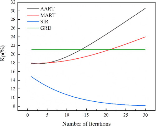
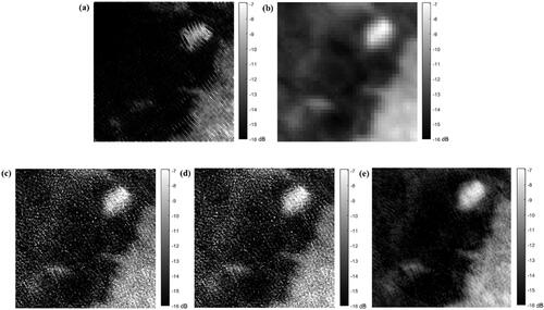
Figure 8 shows that the AART, MART, and SIR algorithms reconstruct the images with the highest accuracy after 3, 6, and 28 iterations, respectively. Figure 9 shows the reconstruction of Hudson Bay using the three algorithms, where Figure 9(a) shows the original backscatter coefficient distribution, Figure 9(b) shows fDIB GRD image, Figure 9(c) shows the image reconstructed with the AART algorithm after 3 iterations, Figure 9(d) shows the image reconstructed with the MART algorithm after 6 iterations, and Figure 9(e) shows the image reconstructed with the SIR algorithm after 28 iterations. In Figure 9, the brighter regions are islands, and the darker regions are sea ice; the backscatter coefficient of the island is significantly higher than that of the sea ice. Many features can be observed in all four images, but the shape of the right island in the SIR image is clearer than in the AART and MART images, and the SIR image contains many fine features. The AART and MART images contain considerable speckle noise, and the SIR image contains almost no high-frequency noise-like artifacts, indicating that the SIR algorithm provides better noise suppression ability than the AART and MART algorithms and can effectively enhance the spatial resolution of the scatterometer data.

Figure 9. Image reconstruction of Hudson Bay by different algorithms. (a) Original backscatter coefficient distribution, (b) fDIB GRD image at 10 km, (c) AART-reconstructed image at 5 km, (d) MART-reconstructed image at 5km, and (e) SIR-reconstructed image at 5 km.

3.2.2. Quantitative analysis of the AART, MART and SIR algorithms

To illustrate the effectiveness of image reconstruction using the SIR algorithm for Hudson Bay, a fDIB GRD image is compared to the images reconstructed with the three different methods previously discussed.

As shown in Table 1, the maximum value of the backscatter coefficient of the SIR image differs from that of the resampled GRD image by 0.7807 dB, and the minimum value differs by 4.1917 dB. The maximum values of the backscatter coefficient of the AART and MART images differ from those of the resampled GRD images by 6.0019 dB and 7.1858 dB, and the minimum values differ by 18.3596 dB and 18.1591 dB, respectively. Thus, compared with the SIR algorithm, these algorithms yield poor reconstruction accuracy. The STD value of the SIR image is the smallest at 2.4771 dB, indicating that the SIR results are superior to those of the other two images, which is consistent with the conclusion reached in the Iceland region. The SIR image is characterized by the smallest information entropy, indicating that the SIR image includes the largest amount of information. Additionally, as shown in Table 2, the SIR image has the strongest correlation with the nonenhanced image, the RMSE of the SIR image is the smallest, and the SSIM of the SIR image is the largest. These results indicate that the SIR image is highly similar to the reference image. Moreover, the PSNR of the SIR image is the largest, which indicates that the distortion between this image and the reference image is the lowest.

The Sentinel-2B data were processed through radiometric calibration, atmospheric correction, mosaicing, and downsampling steps. The SIR images were correlated with Sentinel-2B data, with a correlation coefficient of 0.9988. The results indicate that the reconstructed images highly encompass the features of the optical data in the same area; i.e. the reconstructed islands and sea ice areas display excellent agreement with the actual geographical features in the study area.

4. Discussion

4.1. Other factors affecting image reconstruction

The images obtained with the SIR algorithm display different noise levels for the Iceland and Hudson Bay regions. Notably, the reconstructed image of the Hudson Bay region contains more noise than that of the Iceland region. Figure 10 shows the scatter density plots of the non-enhanced images (i.e. fDIB GRD images) of the Iceland and Hudson Bay regions and the images reconstructed using the SIR algorithm to intuitively illustrate the number of individual pixels deviating from the fit line and the degree of deviation. Cases in which many individual pixels deviate from the fit line indicate high noise in the reconstructed images, and vice versa.

Figure 10. Scatter density plots between images reconstructed with the SIR algorithm and non-enhanced images. (a) Iceland region, and (b) Hudson Bay region.

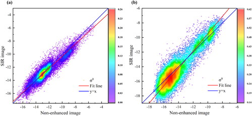
For the Iceland region, the reconstructed backscatter coefficients are more uniformly clustered along the y = x straight line, and for the Hudson Bay region, the backscatter coefficients of the reconstructed images are relatively consistently located along the y = x straight line; moreover, the number of individual pixels that deviate from the fit line is higher in the latter case, indicating that the reconstructed images of the Hudson Bay region are less accurate than those of the Iceland region. The main reasons for these differences are as follows. First, the sampling density and the number of measurements were different in the two regions during the reconstruction process. When reconstructing the Iceland region, the 3-day scatterometer provided 644,554 measurements of the region, and when reconstructing the Hudson Bay region, the 3-day scatterometer provided 391,295 measurements of the region. Based on the reconstruction principle, the higher the scatterometer sampling density is, i.e. the greater the ground coverage areas of adjacent measurements overlap, the better the resolution improvement. Since the amount of data used in the reconstruction of the Hudson Bay region was less than that used in the Iceland region, relatively low spatial overlap occurred in the Hudson Bay region, which ultimately led to poorer reconstruction results in this region compared to those in the Iceland region. By increasing the imaging interval, the number of measurements and the spatial overlap can be increased to improve the reconstruction quality. Second, the surface changes caused by sea ice movement lead to different backscatter coefficients measured in the same area. Since the Iceland region is mainly land, the radar properties of the region remain unchanged during each scatterometer pass; however, the Hudson Bay region is mainly sea ice, and the radar properties of the target region differ over multiple measurements due to sea ice motion, thus influencing the subsequent resolution enhancement to some extent.

4.2. The effective resolution

Due to the variable SRF and measurement spacing, the effective resolution of the reconstructed images may vary across the image. It is therefore difficult to precisely quantify the resolution of the reconstructed images as a single value.

We used Sentinel-2 data with a resolution of 60 m processed by downsampling to correlate with images reconstructed by the SIR algorithm with a resolution of 5 km, and the correlation coefficients were 0.9992 and 0.9988 for the Iceland and Hudson Bay regions respectively, showing that the reconstructed images are highly correlated with features from optical data in the same region in the paper. In addition, the effective resolution will be studied in the future when the appropriate level of data is available.

5. Conclusion

CSCAT is a fan-beam rotary scanning mechanism that combines the advantages of the traditional fixed fan-beam mechanism and the pencil-beam rotary scanning mechanism, with multiple combinations of observation data and high data overlap in polar regions. The application of scatterometers is limited by the data resolution and the principles of new scanning mechanisms. In this paper, we construct a geometric model of the main lobe-to-ground projection relationship based on the detection mechanism of CSCAT and characteristics of CSCAT data and apply it for high-resolution backscatter coefficient-based image reconstruction. The SRF is obtained based on the antenna pattern of CSCAT and the scatterometer backscattering model, and this function is then applied in an image reconstruction algorithm to improve the spatial resolution of image data by taking advantage of the high overlap of scatterometer data coverages. The paper simplifies the SRF for the sake of computational convenience and efficiency, which will entail some losses and how small the loss really is will be further evaluated later.

Image reconstruction is performed based on VV-polarized data using three algorithms: SIR, AART and MART. The results show that the SIR algorithm converges with increasing number of iterations and the normalized standard deviation becomes stable. Additionally, the reconstruction accuracy of the SIR algorithm is higher than that of the AART and MART algorithms. The shapes of land and ice areas in SIR images are clearer than those in AART and MART images, and SIR images contain many fine features. The SIR algorithm displays better noise suppression ability and provides better image reconstruction results.

To further verify the accuracy of the images reconstructed with the SIR algorithm, correlation analysis was performed using Sentinel-2 optical remote sensing data, and the Pearson correlation coefficients of Iceland and the Hudson Bay area were 0.9992 and 0.9988, respectively, indicating that the reconstructed images displayed excellent agreement with the actual geographical features in these areas. Scatterometer-enhanced images may be more effective for large-scale monitoring than images obtained with high-resolution radar sensors due to their wider coverage and lower cost of acquisition. By using image reconstruction techniques combined with CSCAT with high-resolution sensors, studies of land, vegetation and sea ice monitoring can be extended to larger areas.

Acknowledgments

We thank the National Satellite Ocean Application Service for the China-French Oceanography Satellite Microwave Scatterometer L1B data, and the United States Geological Survey (USGS) for the Sentinel-2 remote sensing data..

Disclosure statement

No potential conflict of interest was reported by the authors.

Data availability statement

The data that support the findings of this study are available from the corresponding author upon reasonable request.

Additional information

Funding

This work was supported by the Natural Science Foundation of Shandong Province under grant ZR2022MD002 and the National Key Research and Development Program of China under grant 2021YFC2803300.

References

- Ashcraft IS, Long DG. 2003. The spatial response function of seawinds backscatter measurements. Proc SPIE Int Soc Optical Eng. 5151:609–618.
- Censor Y. 1983. Finite series-expansion reconstruction methods. Proc IEEE. 71(3):409–419.
- Dong X, Zhu D, Lin W, Zhang K, Yun R, Liu J, Lang S, Ding Z, Ma J, Xu X. 2020. Orbit performances validation for CFOSAT scatterometer]. Chin J Space Sci. 40(3):425–431. Chinese.
- Drinkwater MR, Early DS, Long DG. 1994. ERS-1 investigations of southern ocean sea ice geophysics using combined scatterometer and SAR images. Proceedings of 1994 IEEE International Geoscience and Remote Sensing Symposium (IGARSS); p. 165–167.
- Early DS, Long DG. 2001. Image reconstruction and enhanced resolution imaging from irregular samples. IEEE Trans Geosci Remote Sens. 39(2):291–302.
- Gang W, Dong X, Bao Q, Di Z, Xu X. 2015. An unfocused SAR design to improve azimuth resolution of dual-frequency full-polarized scatterometer. Proceedings of 2015 IEEE International Geoscience and Remote Sensing Symposium (IGARSS). p. 4878–4881.
- Gordon R. 1971. A tutorial on ART. IEEE Trans Nucl Sci. 21:78–93.
- Herman GT, Lent A, Rowland SW. 1973. ART: mathematics and applications. J Theor Biol. 42:1–32.
- Kunz LB, Long DG. 2005. Calibrating SeaWinds and QuikSCAT scatterometers using natural land targets. IEEE Geosci Remote Sens Lett. 2(2):182–186.
- Lang S, Lin W. 2017. Comparison of the fan-beam and pencil-beam scatterometers for satellite remote sensing systems. J Ocean Technol. 36(1):19–23. Chinese.
- Lin W. 2011. [Study on Spaceborne Rotating, Range-gated, Fanbeam Scatterometer System] [dissertation]. Beijing: Graduate University Chinese Academy of Sciences (Center for Space Science and Applied Research Chinese Academy of Sciences). Chinese.
- Lin W, Lang S, Zhao X, Liu J, Li X. 2021. Coastal wind retrieval from the China-France oceanography satellite scatterometer. Haiyang Xuebao. 43(10):115–123. Chinese.
- Lindsley RD, Long DG. 2016. Enhanced-resolution reconstruction of ASCAT backscatter measurements. IEEE Trans Geosci Remote Sens. 54(5):2589–2601.
- Liu J, Lin W, Dong X, Lang S, Yun R, Zhu D, Zhang K, Sun C, Mu B, Ma J, et al. 2020. First results from the rotating fan beam scatterometer onboard CFOSAT. IEEE Trans Geosci Remote Sens. 58(12):8793–8806.
- Liu L, Dong X, Li W, Zhu J, Zhu D. 2017. Spatial resolution and precision properties of scatterometer reconstruction algorithms. IEEE J Sel Top Appl Earth Obs Remote Sens. 10(5):2372–2382.
- Liu X, Lin C, Zhang C, Chen X, Ma X. 2021. Inverse distance weighted interpolation algorithm in the application of the visual space temperature field. Mech Electr Eng Technol. 50(7):250–252. Chinese.
- Long DG, Brodzik MJ. 2016. Optimum image formation for spaceborne microwave radiometer products. IEEE Trans Geosci Remote Sens. 54(5):2763–2779.
- Long DG, Daum DL. 1998. Spatial resolution enhancement of SSM/I data. IEEE Trans Geosci Remote Sens. 36(2):407–417.
- Long DG, Early DS, Drinkwater MR. 1994. Enhanced Resolution ERS-1 Scatterometer Imaging of Southern Hemisphere Polar Ice. Proceedings of 1994 IEEE International Geoscience and Remote Sensing Symposium (IGARSS). 1; p. 156–158.
- Long DG, Hardin PJ, Whiting PT. 1993. Resolution enhancement of spaceborne scatterometer date. IEEE Trans Geosci Remote Sens. 31(3):700–715.
- Long DG, Luke JB. 2003. Ultra high resolution wind retrieval for SeaWinds. Proceedings of 2003 IEEE International Geoscience and Remote Sensing Symposium (IGARSS); p. 1264–1266.
- Long DG. 2017. Comparison of SeaWinds backscatter imaging algorithms. IEEE J Selected Topics Appl Earth Observ. 10(3):2214–2231.
- Meier WN, Stroeve J. 2008. Comparison of sea-ice extent and ice-edge location estimates from passive microwave and enhanced-resolution scatterometer data. Ann Glaciol. 48(1):65–70.
- Remund QP, Long DG. 2014. A decade of QuikSCAT scatterometer sea ice extent data. IEEE Trans Geosci Remote Sens. 52(7):4281–4290.
- Spencer MW, Wu C, Long DG. 2000. Improved resolution backscatter measurements with the SeaWinds pencil-beam scatterometer. IEEE Trans Geosci Remote Sens. 38(1):89–104.
- Swan AM, Long DG. 2012. Multiyear Arctic sea ice classification using QuikSCAT. IEEE Trans Geosci Remote Sens. 50(9):3317–3326.
- Wang L, Ding Z, Zhang L, Yan C. 2019. CFOSAT-1 realizes first joint observation of sea wind and waves. Aerospace China. 20(1):20–27.
- Yun T, Dong X. 2015. Study of image reconstruction techniques for spaceborne scatterometer. Remote Sens Technol Appl. 30(3):495–503. Chinese.
- Zhu J, Dong X, Lin W, Zhu D. 2013. Calibration of the Ku-band rotating fan-beam scatterometer using land extended-area targets. J Electron Inform Technol. 35(8):1793–1799. Chinese.
- Zhu YM. 1993. Extrapolation method to obtain a full projection from a limited one for limited-view tomography problems. Med Biol Eng Comput. 31(3):323–324.