MAE-BG: dual-stream boundary optimization for remote sensing image semantic segmentation

Abstract

Deep learning has achieved remarkable performance in semantically segmenting remotely sensed images. However, the high-frequency detail loss caused by continuous convolution and pooling operations and the uncertainty introduced when annotating low-contrast objects with weak boundaries induce blurred object boundaries. Therefore, a dual-stream network MAE-BG, consisting of an edge detection (ED) branch and a smooth branch with boundary guidance (BG), is proposed. The ED branch is designed to enhance the weak edges that need to be preserved, simultaneously suppressing false responses caused by local texture. This mechanism is achieved by introducing improved multiple-attention edge detection blocks (MAE). Furthermore, two specific ED branches with MAE are designed to combine with typical deep convolutional (DC) and Codec infrastructures and result in two configurations of MAE-A and MAE-B. Meanwhile, multiscale edge information extracted by MAE networks is fed into the backbone networks to complement the detail loss caused by convolution and pooling operations. This results in smooth networks with BG. After that, the segmentation results with improved boundaries are obtained by stacking the output of the ED and smooth branches. The proposed algorithms were evaluated on the ISPRS Potsdam and Inria Aerial Image Labelling datasets. Comprehensive experiments show that the proposed method can precisely locate object boundaries and improve segmentation performance. The MAE-A branch leads to an overall accuracy (OA) of 89.16%, a mean intersection over union (MIOU) of 80.25% for Potsdam, and an OA of 96.61% and MIOU of 86.63% for Inria. Compared with the results without the proposed edge optimization blocks, the OAs from the Potsdam and Inria datasets increase by 5.49% and 7.64%, respectively.

Keywords:

• Deep learning
• Boundary optimization
• Squeeze and excitation
• Semantic segmentation
• Remote sensing

1. Introduction

Remote sensing provides an essential and indispensable method for observing the Earth. Remote sensing image interpretation plays a vital role in many applications, such as land use monitoring and analysis (Fang et al. 2018; Weiss et al. 2020), scene classification and retrieval (Gu et al. 2019; Li Y et al. 2021), building extraction (Gu et al. 2019; Shunping and Shiqing 2019), urban planning (Liu F et al. 2016), road detection (Caltagirone et al. 2017) and building damage classification (Nex et al. 2019).

Recently, various deep learning (DL) architectures have emerged (Zhu et al. 2017) and been applied in semantic segmentation (Hafiz and Bhat 2020), instance segmentation (Alhaija et al. 2017), and target detection (Nasrabadi 2013). Among them, convolutional neural networks (CNNs) (LeCun et al. 1989) have been widely used for analysing visual imagery and have mostly outperformed traditional methods (Yuan X et al. 2021). However, semantic segmentation of remote sensing imagery still faces many challenges. DL applications involving remotely sensed images differ from those involving natural images; remotely sensed images usually have more complicated and diverse patterns, as well as richer spatiotemporal and spectral information. Thus, higher requirements are imposed on the associated processing methods (Yuan Q et al. 2020). For instance, compact land object boundaries are often expected for artificial objects. However, adjacent land classes have spectrally similar appearances, for example, the overlapping grass on the trees and flowerbeds in Figure 1 (a) and (b), are often undistinguishable due to the weak boundaries among objects. Deeper neural networks with continuous convolving and pooling operations have achieved success in the most segmentation and classification tasks (Kunihiko et al. 1982; Yu D et al. 2014). However, accompanied by smooth responses from high-level layers, the operations also incur losses regarding the spatial relationships between the target and surrounding pixels. The edge pixels between classes are blurred, resulting in poor edge preservation in the final segmentation results. As shown in Figure 1, the segmentation results of U-Net (Ronneberger et al. 2015) and Visual Geometry Group 16 (VGG-16) (Simonyan and Zisserman 2014), which involve pooling layers, often suffer from poor boundaries.

Figure 1. For segmentation results of various CNNs, special attention should be given to their performance over the boundaries of land objects. (a) and (b) the image and ground truth, respectively. (c) and (d) Outputs and boundary outputs of FCN-32. (e) and (f) The outputs and boundary outputs of U-Net. (g) and (h) Outputs and boundary outputs of VGG-16.

Previous works have adopted edge extraction to optimize semantic segmentation. Generally, the design process of semantic segmentation enhances the edge features of the given feature map, resulting in a dual network. The two-stream CNN structure presented in Takikawa et al. (2019) treats shape information as a separate branch, uses gated convolutional layers to process boundary-related information, and uses atrous spatial pyramid pooling (ASPP) for fusion. The high-level feature map output from a semantic segmentation network was decoupled into topic features and boundary features in Li Xiangtai et al. (2020), followed by a loss-supervised final reconstruction process. The semantic boundary detection method proposed in Li Xiangtai et al. (2020), Zhen et al. (2020) is a multilabel task that aims to identify the class of pixels belonging to the target boundary. The quality of the edge map is directly related to the amount of supportive information it carries into the subsequent processing stages of the approach (Martin et al. 2004). In summary, these methods use similar dual-stream structures, and the extracted edge responses are tuned by the backpropagation algorithm. The propagated information is derived from a defined loss function measuring the inconsistency between the predicted segmentation map and the ground truth. Therefore, the quality of object borders also highly depends on the quality of the ground truth.

The uncertainties introduced by inaccurate ground-truth labels have also gradually been noticed in recent years (Marmanis et al. 2018). As shown in Figure 1 and Section 5.5, the ground-truth pixels annotated by human beings often have higher uncertainties along object boundaries than pixels in objects. When the training labels near boundaries are unreliable, the predicted segmentation results can only roughly localize objects but cannot precisely describe their boundaries.

In this context, a new challenge is how to obtain semantic objects with accurate boundaries in the case of the ground truth with less accurate boundary delineation. Therefore, we propose a dual-branch framework called MAE-BG. Based on coupling the bottom-up multiscale edge feature map from the MAE branch and the positioning capacity of the smooth branch, the edge information at the lower levels and the semantic information at the top levels are fully utilized. A high-level illustration of the proposed MAE-BG model is shown in Figure 2.

Figure 2. Two instances of the MAE-BG network. BG: The process of gradually integrating the boundary information obtained in the MAE network into the smooth network.(a) The combination of the MAE branch and smooth network as a DC structure. (b) The combination of the MAE branch and smooth network as a Codec structure. The dotted lines represent branches with edge information.

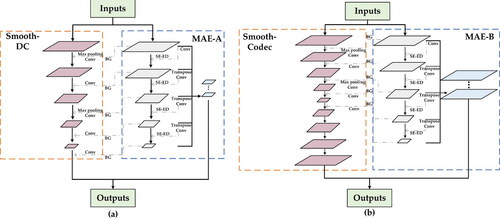
The MAE branch, consisting of multiple squeeze-and-excitation edge detection (SE-ED) blocks, can effectively enhance edge information while extracting edge information at multiple scales. Multiscale edge filters probe the original image, thus capturing objects at multiple scales as well as useful edge information. The main stem of a smooth branch is a typical CNN structure for segmentation. The smooth network utilizes a top-down stage to transmit the context information from high to low stage, ensuring inter-class consistency (Yu C et al. 2018). The multiscale edge maps captured from the ED network are fed into the backbone of the smoothing branch, resulting in a smoothing branch with boundary guidance (BG). Multiple edge localization yields accurate semantic segmentation results and possesses the ability to recover object boundaries at the detail level. To practically fit typical deep convolutional (DC) and encode–decode (Codec) structures of the smooth branch, max pooling and transpose layers are involved in the MAE branch, resulting in two instances of MAE: MAE-A (Figure 2a) and MAE-B (Figure 2b).

We have built a dual-stream network MAE-BG to address weak boundaries and uncertainties introduced by growth truth. The multiscale BG of the smooth network and the multiscale edge extraction of the ED network make the model more robust. In the face of inaccurate ground-truth boundary pixels, the network can still obtain sound boundary localization information. In addition, the problem that edge detail information is lost by continuous pooling operations in deep CNNs (DCNNs) and Codec structure networks is addressed. A comprehensive experimental evaluation of multiple model variants is conducted and reports state-of-the-art results on two challenging segmentation tasks. Experiments show that our network can aggregate multiscale edge information and mitigate the edge effect of classical networks with transplantable performance.

To better distinguish between the edge information obtained in the two networks, the underlying discontinuous edge with a gradient metric is called the ‘edge’. The border of a land object is called the ‘boundary’. The boundaries are carried into the subsequent processing stages for guidance in the smooth branch.

The rest of the paper is organized as follows. Section 2 reviews related works concerning the semantic segmentation of remote sensing imagery. In Section 3, we describe the model architecture in detail. Section 4 describes the dataset used for training and testing the algorithm and provides an experimental analysis to evaluate the model’s generalization ability. Section 5 discusses the experimental results, and the model is summarized and discussed. The method for calculating the two values in this article has been uploaded to https://github.com/970825548/MAE-New.git.

2. Related work

In recent years, semantic segmentation has been widely used in various tasks and has provided a bridge for achieving advanced tasks (Haibo et al. 2017). Typical approaches to remote sensing image semantic segmentation include Markov random fields (MRFs, Zheng et al. 2017), random forests (Kavzoglu 2017), and support vector machines (SVMs, Mitra et al. 2004). As the resolution of satellite images increases, more relevant information becomes available, and an increased number of nonrelevant details emerge (Benediktsson et al. 2012). New challenges for analysing a large number of images at higher spatial details have motivated many new studies. Most studies in recent years have used DL-based approaches to accurately label each pixel as a specific class (Yang H et al. 2019).

With the proposal of fully convolutional networks (FCNs, Long et al. 2015) in 2015, dense predictions of images can be made without a fully connected layer. Sherrah and Sun (Sherrah 2016; Sun and Wang 2018) applied FCN to the semantic segmentation of the high-resolution ISPRS aerial dataset. Sun proposed the MFS to produce improved FCN results by combining semantic details. CNNs have attracted increasing attention in hyperspectral (HS) image classification have attracted increasing attention in hyperspectral image classification. Due to their ability to capture spatial–spectral feature representations. However, their ability to model the relationship between samples is still limited. Therefore, graph convolutional networks (GCNs) have recently been proposed and successfully applied to semantic segmentation (Hong et al. 2020). The residual network (ResNet) (He et al. 2016) uses a short connection to solve gradient explosion and gradient disappearance problems. Wang et al. 2018) used ResNet and ASPP as encoders and combined high-level and low-level features as decoders to obtain multiscale contextual information and clear object boundaries. The Codec structures of the segmentation network (SegNet) and U-Net (Ronneberger et al. 2015; Badrinarayanan et al. 2017) have also achieved excellent results. SegNet is mainly characterized by preserving the maximum indices in the max pooling process of its encoder and using these indices for nonlinear upsampling in the decoder layer. U-Net, on the other hand, adopts a jump-splicing connection architecture to input the relevant features lost in the encoder pooling process into the decoder to maximize the feature retention ability of the network. The VGG network was proposed in 2014. The main contributions of this network are that it achieves improved performance from the perspective of network depth by deepening the network structure and reducing the complexity of training by shrinking the number of weights in the network with small filters. The associated paper improved a CNN and evaluated images obtained with different network depths in detail, demonstrating that the depth of a network plays a significant role in improving performance. Due to their strong generalization capabilities, VGG-16 and VGG-19 perform well in semantic segmentation and object detection tasks. CCR-Ne (Wu et al. 2021) is proposed to learn classification through a cross-modal reconstruction strategy by exchanging information with each other in an efficient way. The use of CCR allows the features of different modalities obtained by the CNN extractor to be fused in a more compact manner. This further demonstrates the effectiveness and superiority of the proposed CCR-Net in classification tasks.

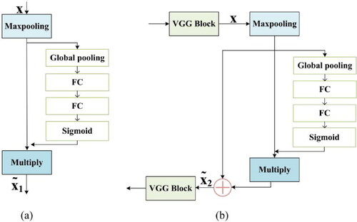
An attention mechanism is a module that allocates computational resources to more important tasks when the available computational power is limited. In neural network learning, the more parameters a model has, the more expressive the model is and the more information the model stores. However, this can bring about information overload problems. Therefore, an attention mechanism can be introduced to focus on the information that is more critical to the current task among the many input data while paying less attention to other details or even filtering out irrelevant information. This mechanism can solve the information overload problem and improve task processing efficiency and accuracy. Hu et al. (2018) proposed a new structural unit called the ‘squeeze-and-excitation’ block. It adaptively recalibrates the channel characteristic response by modelling the mutual drop between channels. These SE blocks are stacked together to form the SE network.

Conditional random fields (CRFs) and MRFs (Sutton and McCallum 2012; Wang et al. 2017) have been used to capture fine edge details. However, CRFs mainly rely on low-level and local information, which exhibits uncertainty regarding its effect on enhancing semantic segmentation results. Holistically nested edge detection (Hed) (Xie and Tu 2015) is a multiscale and multilevel network structure used for target and ED. They proposed a boundary-guided CNN to extract buildings from high-resolution remote sensing images. Their method uses a subnetwork formed by the fusion of two layers extracted from the structure of VGG-16 for better use of edge information. The Hed or BG approaches have been explored in many works (Liu Y et al. 2018; Marmanis et al. 2018; Jung et al. 2021; Yang et al. 2022). Marmanis et al. (2018) constructed a relatively simple, memory-efficient model by adding boundary detection to the SegNet encoder-decoder architecture. Experimentally, boundary detection significantly improves the semantic segmentation ability of CNNs in an end-to-end training scheme. Liu et al. (2018) performed multifeature fusion with ScasNet, using VGG to extract the edge information and then fusing it with the feature output of the decoder. Yu et al. (2018) used a border network in the encoder and a smooth network in the decoder. The network utilizes its border network to expand the interclass distinctions among features. It allows high-level semantic information to refine low-level detailed edge information through a bottom-up design. Jung et al. (2021) proposed a method to integrate Hed, which extracts edge features via the encoder of a given architecture. Experiments showed that this method performed better than competing approaches on five different datasets (DeepGlobe, Urban3D, WHU (HR, LR), and Massachusetts). Some methods use edge and smooth networks with multiscale fusion features (Liu et al. 2018; Yu et al. 2018). The dual-stream network in the existing method can extract most of the features though. However, the commonly used backbone network employed in the segmentation process is not able to fully utilize the multispectral image texture features. And the generalization performance of ED network branches is not high also the network does not have portable performance. In contrast, our ED network is small, has strong performance and can be ported to different networks to obtain accurate edge features through multiscale localization and constant correction of edge information.

3. Methodology

This section describes the proposed MAE-BG approach in detail. Section 3.1 presents the building block (SE-ED) of the MAE branch, and Section 3.2 presents the dual-stream networks.

3.1. The building block of the MAE branch

An MAE network consists of multiple SE-ED combinations. The SE-ED structure is inspired by the SE block. We improved the SE block by using skip connections and then applied it to feature edge extraction. We also considered placing the modified SE block in the backbone network and observing if a gain was produced. It is demonstrated experimentally that using this squeeze and excitation mechanism does not filter out distinguishable category features in the segmentation process. Instead, it suppressed the desired features, leading to a decrease in the accuracy of segmentation.The proposed SE-ED block applies its squeeze-and-excitation mechanism to the edge extraction process to enhance the weak edge information and suppress the clutter texture information generated by other factors during edge extraction.

The purpose of the SE block (in Figure 3.a) is to ensure that the network can improve its sensitivity to relevant features and suppress irrelevant features. This goal is achieved in two steps. As shown in (1), the first step is the squeezing step (global information embedding), where each channel generates channel information using global pooling. The second step is excitation (active calibration), which acquires the linkages between the channels as in (2). After the above process is completed, the weight of each channel in the input feature graph U is obtained. Finally, the weights and the original features are combined by multiplication, as in (3). (1) $$z_c\mathrm{ }=\mathrm{ }{F}_{sq}{u}_{\mathrm{c}})\mathrm{ }= \frac{1}{H\times w}{\sum }_{i=1}^H{\sum }_{j=1}^W{u}_c(i, j).$$(1) where U $\mathrm{ }\in \mathrm{ }{R}^{H\times W\times C}$ denotes the feature maps, and the outputs U = [$u_1,$ $u_2,$…, $u_C$], so $u_C\mathrm{ }\in R^{H\times W}.$ (1) expresses U through its spatial dimensions H×W. (2) $$s = F_{ex}(z, W) = \sigma \left(g \right(z, W) = \sigma (W_2\delta \left(W_{1}z\right)).$$(2)

Figure 3. The MAE branch of the MAE-BG network, consisting of multiple SE-ED blocks. (a) the original SE block, and (b)multiple SE-ED blocks used in our MAE branch. FC the fully connected layer, x denotes the inputs, $\widetilde{X_1}$ the output of the SE block, and $\widetilde{X_2}$ the output of the SE-ED block.

In (2), $\delta$ refers to the rectified linear unit (ReLU) activation function, z is the global description obtained by the squeeze operation, and $W_1\mathrm{ }ϵ\mathrm{ }{R}^{\frac{C}{r}\times C},$ ${\mathrm{ }W}_2\mathrm{ }ϵ\mathrm{ }{R}^{C\times \frac{C}{r}}.$ Here, r is a scaling parameter mainly used to reduce the network's computational complexity and the number of parameters. (3) $$\widetilde{X_1}=F_{\mathit{multiply}}\left(u_c,s_c\right)=\mathrm{ }{s}_c{u}_c,$$(3) (4) $$\widetilde{X_2}=\mathrm{ }{F}_{\mathit{multiply}}\left(u_c,s_c\right)+\text{ M }\left(u_c\right),$$(4) where $\widetilde{X_1}$ = [$\widetilde{x_1},$ …, $\widetilde{x_C}$] and $F_{\mathit{scale}}\left(u_c,{\mathrm{ }s}_c\right)$ refers to channelwise multiplication between the scalar $s_c$ and the feature map $u_c$∈$R^{H\times W}$ in (3). In (4), M ($u_c$) is obtained by pooling the input feature maps. $\widetilde{X_2}$ is obtained by numerical summation of $\widetilde{X_1}$ and M ($u_c$), which is only numerical summation and does not change the channel dimension.

Due to these properties, SE blocks are often used for scene classification. However, the information of small targets, such as cars and small bushes, can easily be judged as unnecessary during segmentation, leading to wrong segmentation results. . Therefore, instead of adding the SE block to the smooth network, our method adds the SE-ED block to the edge network (in Figure 3. b). In addition to the SE block, shortcut connections are used (such as the SE-ResNet structure) to better reform edge features, as in (4). Using the SE-ED block improves the sensitivity of edge features and suppresses the unnecessary features generated when extracting edge information. The SE-ED block is merged with the edge extraction method.

The Hed network can fuse edge information by pooling multiple scales. By adding the SE-ED block, the network can fuse multiscale information while enhancing weak edges, such as vehicles, and suppressing cluttered texture information, such as low vegetation. The Hed network extracts edge features via continuous downsampling to achieve multiscale feature extraction.

In this paper, MAE is mainly used to solve the problem of image edge extraction and prediction. The MAE network shown in Figure 4 retains the basic structure of VGG with the fully connected layer removed. The network uses multiscale and multilevel feature learning. The algorithm accomplishes prediction in an image-to-image manner through DL models. More specifically, the details in ED are obtained by the rich hierarchical features learned. As shown in Figure 4, the structure uses VGG-16 as a backbone, and the last convolutional layers of all groups of VGG-16 are output and then fused. Based on the improved FCN and VGG, six losses are simultaneously induced to optimize the training process, and multiple side outputs produce edges of different scales.

Figure 4. The MAE branch of the MAE-BG network, consisting of multiple SE-ED blocks.

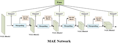
Then, a trained weight fusion function obtains the final edge output. The ambiguity of edges and object boundaries can be solved. Our network refers to these convolutional layer structures as VGG Block1, VGG Block2, VGG Block3, VGG Block4, and VGG Block5. After the convolution process, a side branch is extracted from each VGG block as the output. Then, the output obtained by downsampling and the SE-ED block is fed to the next VGG block simultaneously. This approach amplifies the edge features, and the undesired textures are suppressed once before extracting the next side branch output. Finally, all branch outputs are restored to the same size by pooling, transposition, and 1 × 1 convolution layers, and then multiscale fusion is achieved by layer stacking to obtain the fused image.

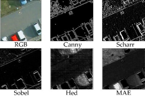
Figure 5 shows the differences between several typical edge operations and our approach. Commonly used ED algorithms include Canny (1986), Sharma and Mahajan (2017), and Vincent and Folorunso (2009). These approaches have more connected broken lines due to local brightness and data noise. Many incorrect texture cues and improperly fused feature maps cannot play a guiding role in the segmentation process and make the results terrible.

Figure 5. Result comparison of typical ED operators. The first row, from left to right and from top to bottom, the original RGB image and the edge maps obtained by Canny, Scharr, Sobel edge detectors, the Hed network and the proposed MAE branch.

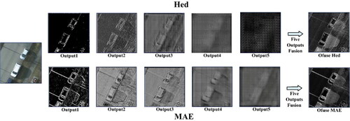
Figure 6 shows the boundary extraction processes of the Hed network and MAE network. Due to the abstraction of feature pooling, the results of Output4 and Output5 exhibit more ambiguous states. After adding the SE module, both the output of the single layer of the VGG block and the edge features are obtained after performing fusion. The edge extraction effect is better than that of the original Hed network. The output of each stage of the Hed network is visible after the addition of the SE-ED block, and the fine and cluttered background information is suppressed. Comparing the fused images of the two networks, the image obtained with the SE-ED block better retains the texture details.

Figure 6. The edge outputs of the Hed network before and after adding the SE-ED block (for better presentation, all fused images are rescaled to the same size). The first row contains the outputs of the five stages of the Hed network, and the second row contains the outputs of the five stages of the MAE network.

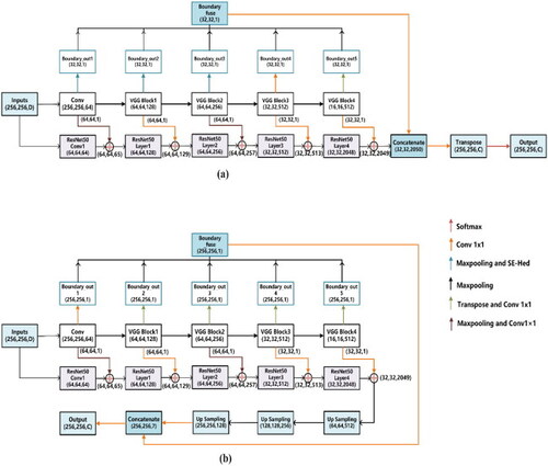
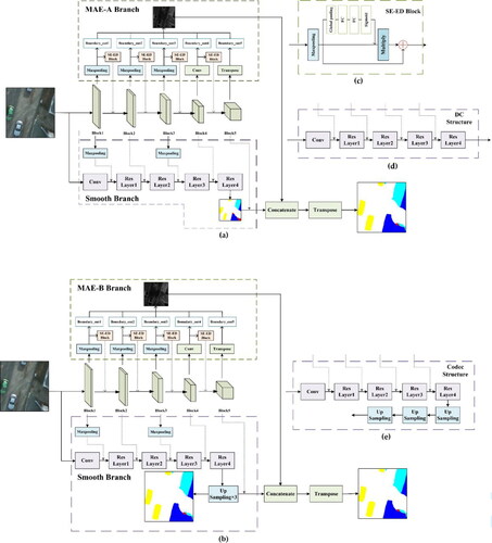
In Figure 7 (d) and (e), we show two smooth network structures that can be added to our proposed MAE network. Taking the layers in ResNet as an example, MAE can be combined with a DC and can also be used with Codec networks. Figure 7(d) shows the DC smoothing network combined with our MAE-A network, and Figure 7(e) shows the Codec structure combined with MAE-B. The specific combinations are described in Section 3.2.

Figure 7. The detailed MAE-BG network infrastructures, containing the smooth branch and the MAE. (a) The dual-stream network for a typical segmentation main stem with a DC structure. (b) Dual-stream network for segmentation of the main stem with the Codec structure. (c) The SE-ED block in the MAE branch. (d) Detailed DC-structure smooth branch combined with MAE-A. (e) Detailed Codec-structure branch combined with MAE-B.

3.2. Dual-stream MAE-BG network with MAE and smooth branches

This paper uses a two-stream MAE-BG network for RS image segmentation. The two networks are the smooth network and the MAE network. Figure 7 shows the two ways of combining the MAE-A and smooth branches in the MAE-BG network. The smooth branch improves ResNet and adds BG to each ResNet layer to achieve boundary localization in high-level semantic information.

Figure 7(a) shows how the MAE-A and smooth branches are merged for a DC structure. The smooth branch extracts the high-level semantic information through a deep neural convolutional process with continuous downsampling. The edge feature map of MAE-A is fused with the feature map of the smooth network and then transposed to recover the resolution of the feature map. Figure 7(b) shows how the MAE-B and smooth branches are merged for a Codec structure. The smooth branch extracts the features through encoding and decoding and then recovers the image resolution. The MAE-B branch uses the transposition method to recover the edge feature map. Finally, the edge feature map output by MAE-B is merged with the feature map output by the smooth network.

The backbone of the smooth network includes the four Res layers of ResNet-50. The VGG block in the MAE network guides the ResNet layers by pooling and 1 × 1 convolution generation while the boundary is obtained. The VGG block in the MAE network also generates feature information to guide the ResNet layers through pooling and 1 × 1 convolution. First, multiple bands of RS images are fed into the dual-stream network. The Potsdam data are processed without any special nDSM band treatment, and only a simple channel stacking operation is performed. The semantic-scale network is constructed here using nDSM to allow trees with significant height information and low vegetation to be more separate. The inputs of both the MAE and smooth branches contain four channels. Each block is extracted twice. Two edge extraction methods are used for Block1. For the first edge extraction step, Block1 extracts the out1 boundary after max pooling and superimposes the edge information obtained by the SE-ED block with the output of max pooling as the input of Block2. For the second edge extraction step, Block1 is channelwise merged with the output of the convolutional layer of ResNet-50 by max pooling and 1 × 1 convolution. Block2 also has two edge extraction methods. For the first edge extraction process, Block2 extracts the out2 boundary after max pooling while superimposing the edge information obtained by the SE-ED block with the output obtained after max pooling as the input of Block3. For the second edge extraction procedure, Block2 is channel merged with the output of Res Layer2 of ResNet-50 by 1 × 1 convolution. Two edge extraction methods are also applied for Block3. Block3 extracts the out3 boundary after max pooling for the first edge extraction process. In contrast, the edge information obtained by the SE-ED block is superimposed with the output obtained after max pooling as the input of Block4. For the second edge extraction process, Block3 is channelwise merged with the output of Res Layer2 of ResNet-50 by max pooling and 1 × 1 convolution. Two steps are involved in the Block5 edge extraction method. Block5 extracts the out5 boundary after transposition for the first edge extraction step. In contrast, the edge information obtained by the SE-ED block is superimposed with the output obtained after max pooling as the input of Block5. For the second edge extraction process, Block5 performs channel merging with the output of Res Layer4 of ResNet-50 via 1 × 1 convolution. This output is concatenated with the output of ResNet-50, recovering the feature image size by upsampling. These five blocks are crucial in a two-stream network. In the above way, multiscale edge extraction and constant edge localization are achieved. The smooth networks of (a) and (b) are both ResNet-50s in Figure A1. The input image is a stacked RGB and nDSM image with four channels. The MAE network fuses 5 ‘out’ boundaries into a (32, 32, 1) boundary via max pooling and transposition. Then, this output is concatenated with the output of ResNet-50 as (32, 32, 1026) and finally transposed together into the original image features. The MAE network in Figure A1. (b) fuses 5 ‘out’ boundaries into one (256, 256, 1) boundary via 1 × 1 convolution and transposition.

This section describes the parameter settings used for the two main architectures in the dual-stream network, VGG and ResNet. Here, f is the number of output channels (or features; the input number of features is deduced from the previous layers), k is the convolution kernel size, d is the dilation rate, and s is the stride of the convolution operation. In all convolution operations, we use appropriate zero padding to keep the dimensions of the produced feature maps equal to those of the input feature map (padding=‘same’). The layers with # in the table are variable, and max pooling or transposition settings depend on the desired feature map size.

The parameters of the blocks are the same as those of the VGG block in the ED network. VGG Block1 and VGG Block2 are composed of two Conv2D layers, and VGG Block3 and VGG Block4 are composed of three Conv2D layers. The method uses ResNet as the main framework with five convolution layers, as shown in Table 1. The first convolution layer possesses a kernel size of 7 × 7 and utilizes max pooling with a kernel size of 3 × 3 and a stride of 2. The second and third layers each consist of three ‘bottleneck’ building blocks with strides of 2. The fourth and fifth convolution layers consist of 23 and 3 ‘bottleneck’ building blocks, respectively, and their strides are 1. Compared with the original network, the stride size applied for the last two layers changes from 2 to 1, and the output shape of the feature map changes from (8, 8, 2048) to (32, 32, 2048). Taking the smooth network combined with DC as an example, we show the detailed parameter settings of the MAE-BG structure in Table 2. We input the extracted edge information from Blocks 1–5 into the MAE branch to obtain the edge features. At the same time, we input it into the smooth branch for another boundary localization.

Table 1. Details of the MAE network parameters.

Layer	Layer type
1	Conv2D (f = 64, k = 7, s = 2)×2
2	Basic Block (f = 64, k = 3, s = 2) ×3
2	Conv2D (f = 64, k = 3)×2
Res Layer2	Basic Block (f = 256, k = 3, s = 2) ×4
Res Layer3	Basic Block (f = 256, k = 3, s = 1) ×6
Res Layer4	Basic Block (f = 512, k = 3, s = 1) ×3

Table 2. Details of the MAE-BG.

Layer	Layer type
1	Block1
2#	Max pooling (Layer1), Conv2D 1 × 1
2	Max pooling (Layer1, s = 2)
3	SE-ED Block (Layer2#)
4	Block2 (Layer2 + Layer3)
5#	Max pooling (Layer4), Conv2D 1 × 1
5	Max pooling (Layer4, s = 2)
6	SE-ED Block (Layer5#)
7	Block3 (Layer5 + Layer6)
8#	Max pooling (Layer7), Conv2D 1 × 1
8	Max pooling (Layer5, s = 2)
9	SE-ED Block (Layer8#)
10	Block4 (Layer8 + Layer9)
11#	Conv2D 1 × 1 (Layer10)
11	Max pooling (Layer5, s = 2)
12	SE-ED Block (Layer11#)
13	Block5 (Layer11 + Layer12)
14#	Transpose (Layer13)
15	SE-ED Block (Layer14#)
16	Conv2D 1 × 1 (Layer16)
17	Sigmoid

4. Experimental settings

4.1. Dataset

This section reports the two datasets employed for evaluation, the detailed implementation and the utilized accuracy assessment method.

4.1.1. ISPRS 2D semantic labelling contest Potsdam dataset

The ISPRS 2D semantic labelling contest Potsdam dataset (International Society for Photogrammetry and Remote Sensing. 2Dsemantic labeling contest. Accessed: March 20, 2020. [Online]. Available:http://www2.isprs.org/commissions/comm3/wg4/semantic-labeling.html) (https://www.isprs.org/education/benchmarks/UrbanSemLab/2d-sem-label-potsdam.aspx) is a high-resolution aerial image dataset (shown in Figure 8.a). This dataset has 38 images with the same size (6000 × 6000 pixels) and a spatial resolution of 0.5 metres.

Figure 8. Two datasets used for experiments. (a) ISPRS 2D Semantic Labelling Contest Potsdam dataset and (b) Inria Aerial Image Labelling dataset.

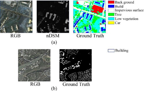
The image files are composed of different channels, including IRRG (3 channels, IR-R-G), RGB (3 channels, R-G-B), (1 channel, nDSM), and DSM channels (one channel, DSM). In this experiment, RGB images are combined with nDSM images. To address the edge improvements achieved by the proposed methods, we do not perform any special treatment on the nDSM band; we directly stack it with 3 spectral channels, resulting in images with 4 channels. The dataset contains 38 RS patches (6,000 × 6,000), and each patch is extracted from orthophoto images, among which 24 images have the corresponding semantic labels. The images contain 6 classes: background, buildings, impervious surfaces, trees, low vegetation, and cars.

Therefore, 24 images are used in the training set and validation set. These twenty-four images are augmented to 32,000 images. When 15 images are used for training, one image is used for validation. There are 29,120 training and 2,080 verification image patches.

4.1.2. Inria aerial image labelling dataset

The Inria Aerial Image Labelling dataset (Maggiori et al. 2017) contains high-resolution RS data for several areas in Austin, Chicago, Kitsap County, West Tyrol, and Vienna. Each area has 36 orthophotos with sizes of 5,000 × 5,000 and RGB image band combinations (shown in Figure 8b). The semantic labels of this dataset can be divided into architectural and nonarchitectural (background) categories. Each image is cropped into 24 images with sizes of 256 × 256. All the images are flipped horizontally and vertically and then rotated to obtain the final training set. Each area contains 115,200 images. As with the Potsdam data, 1 validation image is used per 15 training images.

4.2. Implementation details

In this experiment, the training equipment used for the DL network includes an 8-core 16-thread Intel i9-9900K CPU, an NVIDIA RTX3090 graphics card, 24 GB of memory, and CUDA11.2. The software environment includes the 64-bit Microsoft Windows 10 operating system, and the development platform is Anaconda 5.2.0. The built-in Python version is 3.8.8. The DL software framework is TensorFlow 2.5.0. The Adam optimizer is used with a 1 × e⁻³ learning rate for a total of 350 training epochs with a batch size of 32. In the experiments, we use Xavier to randomly initialize the transposition layer.

To prevent overfitting, we rely on geometric methods to expand the data. Therefore, each batch of images is always different, and the algorithm does not see the same sample of images in each iteration. In this paper, augmentations are performed twice. The first training dataset augmentation process uses cropping, rotation, Gaussian blur, noise and colour enhancements. The second augmentation step uses the image obtained from the first augmentation process and performs horizontal, vertical, and mirror flips.

Feature normalization is implemented using the mean and standard deviation (std). The mean and std are obtained from the training set and correspond to the four RGB and nDSM bands, respectively. These values are obtained by computing them on the 32,000 images in the training set via standard deviation normalization. During the experiment, inaccuracies in the ground-truth data are found. A similar analysis was conducted by Wu et al. (2021), Xie and Tu (2015). We reannotate the images in the Potsdam validation set to evaluate the bounds obtained by our method in the presence of inaccuracies in the ground-truth data.

4.3. Accuracy assessment

To comprehensively evaluate the performance of the proposed model, the overall accuracy (OA), precision, recall, F1, and mean intersection over union (MIOU) metrics are used to evaluate the experimental results. The above evaluation indices have often been used in previous papers and compared with the recognized semantic word segmentation evaluation indices. The calculation for evaluation is as follows: (5) $$\mathrm{OA}=\frac{\mathrm{TP}+\mathrm{TN}}{\mathrm{P}+\mathrm{N}}$$(5) (6) $$\mathrm{Precision}=\frac{\mathrm{TP}}{\mathrm{TP}+\mathrm{FP}}$$(6) (7) $$\mathrm{Recall}=\frac{\mathrm{TP}}{\mathrm{TP}+\mathrm{FN}\mathrm{ }}$$(7) (8) $$\mathrm{F}1=2\times \frac{\mathrm{Precision}\times \mathrm{Recall}}{\mathrm{Precision}+\mathrm{Recall}}$$(8) (9) $$\mathrm{MIoU}=\frac{1}{\mathrm{k}+1}{\sum }_{\mathrm{i}=0}^{\mathrm{k}}\frac{\mathrm{TP}}{\mathrm{FN}+\mathrm{FP}+\mathrm{TP}}$$(9) where P is the number of positive samples; N is the number of negative samples; TP is the number of correctly predicted positive samples; FP is the number of positive samples predicted to be false; TN is the number of correctly predicted negative samples, and FN is the number of incorrectly predicted negative samples.

5. Results and discussion

In this section, we report and discuss the performance achieved by the proposed method on the ISPRS Potsdam and Inria datasets. Based on these two datasets, we prove and analyse the effectiveness of the proposed network. First, we present the model performance obtained for the Potsdam and Inria datasets and the performance of MAE-BG in Section 5.1. Second, we demonstrate the efficiency of our model with results obtained from other classic networks in Section 5.2. Third, we analyse and compare the results of our network with those of other state-of-the-art networks in Section 5.3. Then, we analysed the generalization performance of the model in Section 5.4. In Section 5.5, we manually relabelled five graphs in the Potsdam test set and analysed the quality of the Potsdam dataset.

5.1. MAE-BG model performance analysis

5.1.1. Edge detail comparison

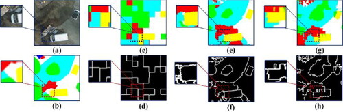
Some of the edge segmentation results are shown in Figure 9. The second row in red indicates the inconsistencies between our segmentation results and ground-truth data (GT). By overlaying these inconsistencies onto the original image, we can observe that inconsistencies with the GT data do not always mean incorrect segmentation results. In many cases, our results fit the original RGB image somewhat better. Furthermore, these inconsistencies in red are partly due to inaccuracies in the manual annotations, such as category marking omissions and nonuniformity between the edges of the GT data and the edges of the original map features.

Figure 9. Comparison between the ground truths and our segmentation results from representative patches of the Potsdam dataset. The first, second and third rows are the original RGB images, the ground truth and our segmentation results, respectively. The fourth row is the red/green image, where green and red indicate correctly and misclassified pixels, respectively. In the fifth row, the red/green image is overlaid on the original images.

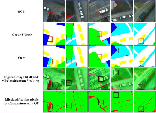
In the first image in the first row (from left to right), the low vegetation in the original picture in the shade is not marked in the GT. The trees and buildings in the second, third and fourth original images do not appear as regularly rounded and right-angled as the hand-labelled versions. Compared with the GTs, the boundaries of our segmentation results match the contours of the real object better, and even the boundaries of cars with skewed rear ends (due to high-speed movements or shooting angles) are more accurately predicted.

5.1.2. Ablation study on the network architecture

In this section, we design experiments with five methods to evaluate the performance of the various modules we use in the MAE-A and MAE-B networks. In Figure 10, the settings with data augmentation, MAE-A and BG, perform best on the Potsdam dataset. Our process improves the MIOU metric by 5.46% compared to ResNet without the augmentation approach. The MIOU obtained using augmentation, the MAE-B network, and the BG network is improved compared to the segmentation result of the ResNet-50 network, but the improvement is less than 3.69%. It is clearly seen that the MIOU of both datasets improves but with different magnitude of gain after adding BG. The effect of adding BG on Postdam is better than adding MAE-B on Inria, while the opposite is true on Inria. Therefore, we subsequently chose the MAE-A and BG with the best effect.

Figure 10. MIOUs tested by different network and training combinations on the Potsdam and Inria datasets, where 'Aug’ denotes augmentation, and 'Res’ indicates ResNet-50. 'MAE-A' and 'MAE-B' denote our proposed MAE-A and MAE-B networks, respectively.

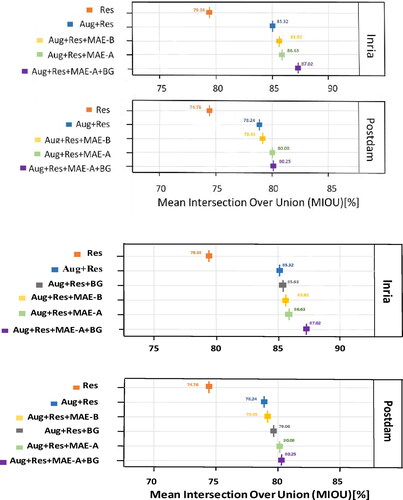
The MAE-B network is slightly worse than the MAE-A network. Therefore, a better way to merge the MAE-B network with the Codec network structure is still worth further exploration. We obtain a 1.84% MIOU improvement after using the primary MAE network with the same augmentation approach. This observation indicates that the MAE network can guide the boundary optimization process and improve the segmentation accuracy.

Similarly, we use a set of experiments with four methods to conduct a validation study on the Inria dataset. The validity of the MAE-A network is mainly verified on the Inria dataset due to the excessive number of parameters used by the MAE-B network when combined with the Codec structure. As shown in Figure 11, the MIOU of our method is improved by 7.64% over that of the original ResNet-50. The MIOU improves by 0.39% after adding edge guidance in the smooth network. The robustness of the edge extraction network is demonstrated by the excellent performance of the MAE network on the two utilized datasets.

Figure 11. Imprecise boundaries in ground-truth data. From top to bottom, the original RGB image, the ground-truth data, our manually handcrafted labels, and the segmentation results obtained by the proposed MAE-BG network.

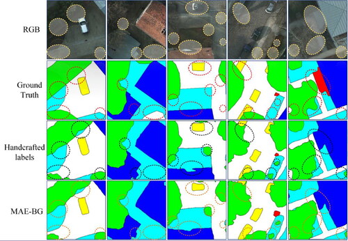
5.1.3. Edge quality analysis of semantic segmentation results

During processing of the Potsdam dataset, we find that the dataset is not fully accurate. In particular, the detected edges of houses and trees often do not correspond to those of the actual boundaries of objects. Then, we carefully and manually label five RGB images in Figure 11 for comparison with the edge result maps obtained by MAE-BG. The comparison shows that the ground-truth data and the handcrafted labels are different. In the ground truth, low vegetation next to trees, the edges of trees, buildings, and clumps of trees overlapping flowerbeds are easily overlooked and mislabelled. The results obtained by our MAE-BG method are not entirely consistent with the handcrafted labels but are closer to the original image in terms of some of the edge details.

5.2. Comparison with classic models

The performance levels of our model and four common models are compared on two datasets. Two deep neural network structures and two Codec neural network structures (four classic networks in total) are chosen for this part. These models are commonly used for segmentation tasks. Due to the uneven numbers of samples in different categories, to conduct a fairer comparison and to better show the effect of our structure in other neural networks, the paper uses the OA, F1 and MIOU metrics for comparison purposes. Table 3 shows the F1 and MIOU scores obtained from the various networks for different categories in the Potsdam test set. The results show that our proposed method outperforms the other models with a total F1 score of 88.78%. The total MIOU score of our model is 80.25%. More specifically, it is difficult to segment categories such as areas with low vegetation, and our network performs better than other networks in this segmentation task. Figure 12. (a) shows the performance achieved by the different networks on the Potsdam test set. Figure 12. (b) We can easily see the low vegetation, which is difficult for multiple networks (VGG-16, U-Net, U-Net, ResNet-50, and ResUNet) to segment. MAE-BG focuses on duplicated extraction of edge improvement trees and low-vegetation segmentation accuracy. Low vegetation and cars with insignificant height information are more clearly segmented from road boundaries, and the edges of buildings are smoother. The above results show that in a case when the edges contained in the ground-truth information are somewhat wrong, we can obtain corrected edge segmentation results even after using the dual edge localization method.

Figure 12. Example semantic labelling output for the Potsdam and Inria datasets using classical networks and MAE-BG trained.

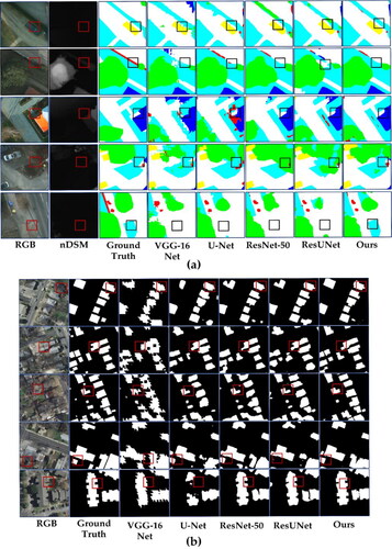
Table 3. F1 and MIOU scores obtained with classic and our models from the Potsdam test set.

	Network	Build.	Imp.S	Tree	Low. V.	Car	Overall
F1	VGG-16	90.14	85.91	69.99	75.41	83.83	81.06
MIOU		82.06	75.30	53.83	60.53	72.17	68.78
F1	U-Net	91.79	87.40	74.11	78.58	90.10	84.40
MIOU		84.82	77.62	58.87	64.71	82.00	73.60
F1	ResNet-50	92.74	88.75	77.47	79.45	87.91	85.26
MIOU		86.46	79.77	63.23	65.91	78.43	74.76
F1	ResUNet	92.77	88.38	72.83	78.54	89.61	84.43
MIOU		86.51	79.19	57.27	64.66	81.18	73.76
F1	Ours	95.72	91.70	81.32	84.09	91.15	88.79
MIOU		91.80	84.67	68.52	72.54	83.73	80.25

There are only two categories in the Inria dataset, and the segmentation target is only in clues buildings; the OA and MIOU values are shown in Table 3. The results demonstrate that our model performs better on the Inria test set than the other common networks. In Table 4, we can see that our method has higher accuracy and MIOU values than the other basic methods. Our method has more precise segmentation boundaries for the concave and convex parts of the buildings in the Inria test set.

Table 4. OA and MIOU scores obtained with classic and our models from the Inria test set.

Network	OA	MIOU
VGG-16	95.05	80.76
U-Net	96.81	85.94
ResNet-50	96.49	85.32
ResUNet	96.45	85.32
Ours	96.91	87.02

Table 5 shows the parameters and FLOPs of different networks. We can see that the number of parameters and FLOPs used by the MAE network are relatively small. Experiments show that we are able to extract excellent edges at multiple scales with 14,807,177 parameters. This small network can be directly applied to deep neural network structures and Codec structures to achieve end-to-end boundary smoothing. Therefore, MAE-BG is expected to be effective and fast in terms of extracting edges and correcting edge features with the addition of more advanced networks. Furthermore, this method enables edge localization while the network is performing feature extraction, so postprocessing (the edge smoothing step) can even be omitted when using this method. The performance of our method on both datasets shows that in the case of an awful ground truth, our edge extractor does not strongly depend on GT, giving our segmentation results a clear advantage.

Table 5. Numbers of Parameters and FLOPs Used by Different Networks.

Network	Params	FLOPs(G)
VGG-16	140,983,040	40.40
U-Net	31,035,718	110.00
ResNet-50	23,564,288	50.00
ResUNet	6,288,054	30.10
MAE-A Network	14,807,177	40.20
MAE-B Network	14,811,722	40.20
Ours	72,165,707	174.00

The boundary pixels of each class are not confused, and the segmentation result map is rarely blurred. Even categories such as trees, which are inaccurately labelled in the ground-truth data, yield better category boundaries than the ground-truth data in our method. Our approach can better outline the building boundaries in the Inria dataset, producing excellent segmentation results.

5.3. Comparison with state-of-the-art methods

In this section, we compare the performance of our proposed dual-stream network with that of several (peer-reviewed) representative CNN models. For comparison, we select some networks that are similar to our network, such as ResNet using an improved, lightweight network (FCN) and a network with ED. Marmanis (Marmanis et al. 2018) added boundary detection capabilities to an encoder-decoder structure to extract the boundaries between different semantic categories. Wang et al. (2018) used a deep ResNet and ASPP as encoders and combined high-level features from both scales with corresponding low-level features as decoders in the upsampling phase. Nogueira (Nogueira et al. 2019) trained a dilated network with different patch sizes, allowing it to capture multicontext features from heterogeneous contexts. Zhang (Zhang W et al. 2017) investigated the contributions of individual layers within an FCN and proposed an efficient fusion strategy for the semantic annotation of colour or infrared images and elevations. While processing these different patches, this network provides a score for each patch size that helps define the optimal size for the current scene. The method exploits the multicontext paradigm without increasing the number of parameters while defining the optimal block size based on the training time. Qi (Qi et al. 2020) proposed a replaceable module (an AT block) using multiscale convolution and attention mechanisms as the building block of ATD-LinkNet. Jamie (Sherrah 2016) proposed segmenting high-resolution remote sensing images using a CCN without downsampling, avoiding deconvolution and interpolation, and experiments showed that this technique is preferred over the original FCN.

In Table 6, the OA, F1, and MIOU scores obtained by our method and other methods on the Potsdam test set are shown. After comparing the results of these simple networks and the segmentation networks with ED, it is found that our method can obtain good segmentation results in the simpler networks. Our method boosts the OA to 89.12% and the MIOU to 80.25%. Table 7 shows the OA and F1 values obtained for the six categories by other methods compared with those of our proposed method in the Potsdam dataset. The F1 values of (Wang Y et al. 2018) and (Qi et al. 2020) are higher than those of our method, but their OA and MIOU values are lower than those of our method, where the MIOU of the method in (Qi et al. 2020)differs from ours by 5.94%. Our method performs better than most other methods in categories with significantly high information levels and large scopes (buildings). Tasar (Tasar et al. 2019) uses U-Net as the main framework to segment the dataset using multiple learning. The differences between the classification accuracies of trees and low vegetation and the other classification accuracies are minor. MAE network, we can clearly see that the cluttered boundaries obtained before joining the network are regularized. The result of boundary partitioning is also smoother in the multicategory case, as demonstrated by the U-Net predictions in the last row.

Table 6. Comparisons Among the OA, F1 and MIOU Scores Achieved by Different Methods on the Potsdam Test Set.

Method	OA	F1	MIOU
FCN·H-V (Marmanis et al. 2018)	85.00	–	–
ResNet + ASPP (Wang Y et al. 2018)	88.30	88.80	–
Dynamic (Nogueira et al. 2019)	87.90	–	–
Mutil-Modal (Zhang W et al. 2017)	80.00	81.80
ATD-LinkNet50(Mignotte 2014)	89.00	90.01	74.31
FCN trained with (DST 2) (Sherrah 2016)	84.14	78.36	–
Incremental Learning (Tasar et al. 2019)	84.25	–	–
Our	89.16	88.79	80.25

Table 7. Comparisons Among the F1 and Precision Scores Produced by Different Methods on the Potsdam Test Set.

Evaluation Methods	Network	Build.	Imp.S	Tree	Low. V.	Car	Overall
F1	FCN·H-V (Marmanis et al. 2018)	--	--	--	--	--	--
Precision		96.80	85.20	79.10	85.40	85.40	85.00
F1	ResNet + ASPP (Wang Y et al. 2018)	94.60	88.90	85.30	82.70	91.20	88.80
Precision		91.70	88.10	85.20	77.60	73.90	88.30
F1	Mutil-Modal (Zhang W et al. 2017)	86.00	80.00	69.00	74.00	70.00	81.80
Precision		88.66	80.82	65.31	68.21	84.02	80.00
F1	Dynamic (Nogueira et al. 2019)	--	--	--	--	--	--
Precision		90.32	82.14	67.10	69.49	82.15	87.90
F1	ATD-LinkNet50 (Mignotte 2014)	95.30	91.60	85.00	84.00	94.20	90.01
Precision		95.30	92.00	83.30	88.80	93.50	89.00
F1	FCN trained with (DST 2) (Sherrah 2016)	92.77	88.38	72.83	78.54	89.61	84.43
Precision		90.78	86.52	78.41	83.01	90.28	84.14
F1	Ours	95.72	91.70	81.32	84.09	91.15	88.79
Precision		96.20	91.27	78.92	86.31	90.12	89.16

Our method obtains better OA and MIOU scores due to amplifying important edge features and suppressing noisy background edges in our ED network. Additionally, multiscale edge extraction in the backbone network plays the role of edge relocalization. Therefore, when compared with the commonly used networks, our approach obtains better edge features even though our OA and MIOU are not much higher. Even better accuracy is obtained compared with some of the similar ED and semantic segmentation networks proposed in the literature. Compared with some large networks, our accuracy still needs to be improved. This gap may be due to the widening method, network depth, or parameter adjustment process.

Since the Inria dataset is not used very frequently by the current methods, we choose three methods here to conduct OA and MIOU comparisons with our method. Zhang (Zhang Y et al. 2019) proposed Web-Net, a nested network architecture with dense hierarchical connectivity, to address these problems and designed ultra hierarchical sampling (UHS) blocks to absorb and fuse interlevel feature maps for propagating feature maps between levels. Li (Li Xiang et al. 2019) proposed using U-Net as the main body and inserted a cascade of cavity convolutions performed in the connected part of the Codec to capture features at different scales. Bischke (Bischke et al. 2019) proposed a new cascading multitask loss to solve the problem of maintaining semantic segmentation boundaries in high-resolution satellite images.

The performance achieved by our method and other methods on the Inria test set in terms of the OA and MIOU metrics is shown in Table 8. The MIOU obtained by our method is also significantly better than other methods when their OAs are not much different. Our method is significantly better than the other methods, especially in terms of the MIOU, which can reach 87.02%; this value is 11.44% higher than that of the worst-performing method. This proves that the MAE network is expected to be used for building target detection to achieve improved edge accuracy. Our method is not only valuable for multicategory semantic segmentation but also effective in binary classification.

Table 8. Comparison Among the OA and MIOU Scores Produced by Different Methods on the Inria Set.

Method	OA	MIOU
Web-Net (Zhang Y et al. 2019)	96.14	75.58
UNet-dilation (Li Xiang et al. 2019)	96.81	73.09
MultiTask (Bischke et al. 2019)	93.21	76.76
Ours	96.91	87.02

5.4 Generalization of the MAE network

Table 9 compares the results obtained by multiple networks before and after adding the MAE network, and the evaluation index is MIOU. For a better comparison, the basic neural networks all use the same data processing method as our network. After adding the MAE, the MIOUs of several basic networks are also slightly improved. To better present the edge results obtained on the Potsdam dataset before and after joining the MAE network, we plot the segmentation and edge results in Figure 13. It is evident that the boundaries of the segmentation results are significantly smoother and clearer after adding the MAE network; for example, the edges of the low-vegetation areas on flowerbeds are sharper, and the boundaries of trees are noticeable. Moreover, our method can better identify low vegetation and cars obscured by trees. Compared with the ground truth, the edge features obtained by our method are significantly more accurate than those of the other methods. In the second row of the display, we can see that the building boundaries obtained after using our segmentation method are even closer to those of the original RGB image than the ground truth. Looking at the boundaries obtained after adding the MAE network, we can clearly see that the cluttered boundaries obtained before joining the network are regularized. The result of boundary partitioning is also smoother in the multicategory case, as demonstrated by the U-Net predictions in the last row.

Figure 13. Comparison of the effects and edge effects produced by the common networks on the Potsdam dataset before and after adding the MAE network. The original RGB image; the ground truth; and the results of VGG-16, VGG-16 after adding MAE, U-Net, U-Net after adding MAE, ResUNet, ResUNet after adding MAE, ResNet, and our method (the MAE-BG network) are shown from left to right.

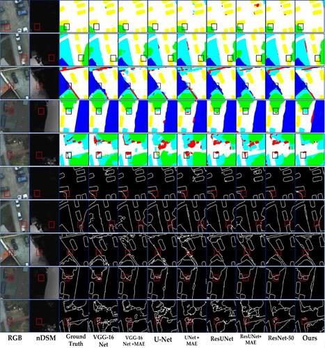
Table 9. The MIOUs Obtained by Classic Networks on the Potsdam set Before and After Joining the MAE Network.

Network	Build.	Imp.S	Tree	Low. V.	Car	MIOU
VGG-16	85.93	78.05	60.34	65.07	76.64	73.21
VGG-16 + MAE	86.62	79.39	62.04	66.29	80.64	75.00
U-Net	88.66	80.82	65.31	68.21	84.02	77.40
U-Net + MAE	88.83	81.42	66.75	68.95	82.68	77.72
ResNet-50	90.32	82.14	67.10	69.49	82.15	78.24
ResUNet	88.33	81.38	65.18	68.93	83.14	77.39
ResUNet + MAE	89.83	81.88	67.17	69.34	80.92	77.83
Ours	91.80	84.66	68.51	72.54	83.73	80.25

Experiments show that the MAE network positively affects several commonly used networks and can act as an edge specification approach. VGG-16 and ResNet-50 are evaluated after adding the MAE-A network. U-Net and ResUNet add the MAE-B network. The MIOU results obtained before and after adding the MAE network (shown in the table) show that the MAE-B network brings a significantly smaller gain than the MAE-A network. Therefore, the combination of the MAE network and the Codec neural network still deserves more discussion, and the space after the combination still needs to be improved.

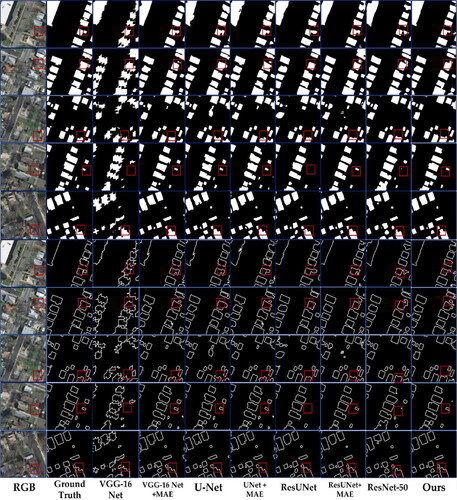
Similarly, Figure 14 compares the segmentation and edge results obtained on the Inria dataset before and after adding the MAE network. The building edges are better after the commonly used networks are added to the MAE network, and even small buildings ignored by the basic networks are more easily detected. Our method even predicts small buildings not shown in the ground-truth data. Our method presents better boundaries when segmenting large buildings. Some tiny buildings, such as those in the RGB image in the fifth row, which the ground truth does not label, have edges that our method can identify.

Figure 14. Comparison of the effects and edge effects produced by the common networks on the Inria dataset before and after adding the MAE network. The original RGB image; the ground truth; and the results of VGG-16, VGG-16 after adding MAE, U-Net, U-Net after adding MAE, ResUNet, ResUNet after adding MAE, ResNet, and our method (the MAE-BG network) are shown from left to right.

6. Conclusion

This study proposes a new dual network MAE-BG trained on image classification to the task of semantic segmentation by applying ED filters for dense feature and multiscale edge extraction. The MAE-BG uses an MAE edge detector branch and a typical smooth branch with BG. The MAE branch incorporates an attention mechanism (SE-ED) to enhance the weak edges that are desired to be preserved and suppress undesirable texture details. To solve the problems arising from inaccurate boundary pixel ground-truth data in the datasets encountered during the segmentation process. Then, our proposed MAE-A and MAE-B networks can be adapted to the DC structure and Codec structure, respectively. The BG step in the smooth branch enables continuous edge localization in high-level semantic information. The network solves the problem of boundary blurring between categories during continuous image pooling to a certain extent.

Then, the generalization ability of the MAE network to mainstream networks is further explored. This lightweight ED network MAE has strong generalization performance and can be integrated easily with other CNNs. Therefore, the MAE networks are expected to be added to more advanced networks for end-to-end edge regularization. We also discuss the limitations of the proposed method, such as its efficiency in capturing edge features when facing Codec networks, which still needs to be improved.

The performance of our framework is evaluated on the 2D semantic segmentation ISPRS Potsdam and Inria datasets. We compare the proposed approach with classic CNN and new segmentation algorithms (similar lighter networks and edge-guided networks). Various computed evaluation metrics have proven the superiorities of the proposed method. Experiments show that MAE-BG does not depend heavily on ground-truth data and still obtains favourable edge results in the case of mislabelling by handcraft. This proves that our proposed scheme is reliable for high-performance semantic segmentation tasks. In the future, we will investigate possible combinations of different deep networks and our MAE-A and MAE-B, and develop more advanced dual-branch networks to fully exploit multi-scale edge details.

Author contributions

Ruiqi Yang: Conceptualization, methodology, writing original draft preparation; Chen Zheng: softerware, supervision, formal analysis, writing-review and editing; Leiguang Wang: conceptualization, resources, validation, writing original draft preparation, writing-review and editing, supervision, funding acquisition; Yili Zhao: formal analysis, investigation, supervision; Zitao Fu: writing-review and editing, funding acquisition, supervision; Qinling Dai: conceptualization, writing-review and editing, funding acquisition, supervision. All authors have read and agreed to the published version of the manuscript.

Abbreviations
Smooth Network	=	The Smooth Network utilizes stage-wise manner to transmit the context information from high to low stage, to ensure the inter-class consistency.
BG	=	Boundary guidance is not a network in this paper. It refers to the process of stage-by-stage and top to bottom integration of boundary information obtained from the MAE network into the Smooth Network.
Hed	=	Holistically Nested Edge Network
SE-ED Block	=	Squeeze-and-Excitation Edge-Detection Block
MAE Network	=	Multiple-Attention Edge Extraction Network
MAE-A Network	=	MAE Network Combined with a DC (Method A)
MAE-B Network	=	MAE Network Combined with a Codec Network (Method B)
ASPP	=	Atrous Spatial Pyramid Pooling
MIOU	=	Mean Intersection-Over-Union

Acknowledgements

We thank ISPRS for providing the Potsdam dataset of airborne data images, which is free and publicly available. For more information, see the official website of the ISPRS Test Project on Urban Classification and 3D Building Reconstruction-2D Semantic Labelling Contest.

Disclosure statement

No potential conflict of interest was reported by the author(s).

Additional information

Funding

This work was supported in part by the National Natural Science Foundation of China under Grants 09910-912123 ,31860182, 32160369, 41961053, and 41771375; in part by the Key Development and Promotion Project of Yunnan Province under Grant 202202AD080010; and in part by the Fund of Reserve Talents for Young and Mid-dle-Aged Academic and Technological Leaders of Yunnan Province under Grant 2018HB026.

Appendix A

Figure A1. The structures of the MAE-A and MAE-B networks and the smooth network they are adapted to. To make the MAE network more practical, a family of ED networks is proposed: MAE-A and MAE-B for deep neural and Codec networks, respectively. D denotes the channel dimensionality of the input, and C denotes the class of the output. Here, we choose a length and width of 256 × 256 as an example. This section proposes two structures for the MAE network: the MAE-A network and the MAE-B network. These two structures allow our ED method to have more robust adaptability to different neural networks. The MAE-A network (as shown in Figure A1.a) is used in DC structure (such as FCN-32, Deeplab v3, VGG and ResNet.). It is first merged with the output of the smooth network and then uniformly upsampled to recover the size of the feature map. The MAE-B network (as shown in Figure A1b) is used with Codec neural networks (such as SegNet, U-Net, and ResUNet). It first recovers the edge feature map and then merges it with the smooth network.

References

- Alhaija HA, Mustikovela SK, Mescheder L, et al. 2017. Augmented reality meets deep learning for car instance segmentation in urban scenes[C]//British machine vision conference. 1:2.
- Badrinarayanan V, Kendall A, Cipolla R. 2017. Segnet: a deep convolutional encoder-decoder architecture for image segmentation. IEEE Trans Pattern Anal Mach Intell. 39(12):2481–2495.
- Benediktsson JA, Chanussot J, Moon WM. 2012. Very high-resolution remote sensing: challenges and opportunities [point of view]. Proc IEEE. 100(6):1907–1910.
- Bischke, B., Helber, P., Folz J., Borth D., Dengel A. 2019. Multi-task learning for segmentation of building footprints with deep neural networks. 2019 IEEE International Conference on Image Processing (ICIP); IEEE.
- Caltagirone L, Scheidegger S, Svensson L, Wahde M. 2017. Fast LIDAR-based road detection using fully convolutional neural networks. 2017 IEEE intelligent vehicles symposium (iv); IEEE.
- Canny, J. 1986. A computational approach to edge detection. IEEE Trans Pattern Anal Mach Intell. PAMI-8(6):679–698.
- Emmanuel Maggiori; Yuliya Tarabalka; Guillaume Charpiat; Pierre Alliez 2017. Can semantic labeling methods generalize to any city? the inria aerial image labeling benchmark. 2017 IEEE International Geoscience and Remote Sensing Symposium (IGARSS); IEEE.
- Fang F, Yuan X, Wang L, Liu Y, Luo Z. 2018. Urban land-use classification from photographs. IEEE Geosci Remote Sensing Lett. 15(12):1927–1931.
- Gu Y, Wang Y, Li Y. 2019. A survey on deep learning-driven remote sensing image scene understanding: scene classification, scene retrieval and scene-guided object detection. Appl Sci. 9(10):2110.
- Hafiz AM, Bhat GM. 2020. A survey on instance segmentation: state of the art. Int J Multimed Info Retr. 9(3):171–189.
- Haibo L, Lingyun X, Bin H, Zheng C. 2017. Status and prospect of target tracking based on deep learning. Infrared Laser Eng. 46(5):502002–0502002. 0502007).
- Hong D, Gao L, Yao J, et al. 2020. Graph convolutional networks for hyperspectral image classification. IEEE Trans Geosci Remote Sensing. 59(7):5966–5978.
- Hu J, Shen L, Sun G. 2018. Squeeze-and-excitation networks. Proceedings of the IEEE conference on computer vision and pattern recognition. 2018:7132-7141.
- International Society for Photogrammetry and Remote Sensing. 2020. 2Dsemantic labeling contest. Accessed Mar. 20 [Online]. Available:http://www2.isprs.org/commissions/comm3/wg4/semantic-labeling.html.
- Long J, Shelhamer E, Darrell T. 2015. Fully convolutional networks for semantic segmentation. Proceedings of the IEEE Conference on Computer Vision and Pattern Recognition. p. 3431–3440.
- Jung H, Choi H-S, Kang M. 2021. Boundary enhancement semantic segmentation for building extraction from remote sensed image. IEEE Trans Geosci Remote Sens. 60:1–12.
- Kavzoglu T. 2017. Object-oriented random forest for high resolution land cover mapping using quickbird-2 imagery. Handbook of neural computation. Academic Press; p. 607–619.
- Kunihiko F, Sei M. 1982. Neocognitron: A selforganizing neural network model for a mechanism of visual pattern recognition. Compet. Coop. Neural Nets. 36:267–285.
- LeCun Y, Boser B, Denker JS, Henderson D, Howard RE, Hubbard W, Jackel LD. 1989. Backpropagation applied to handwritten zip code recognition. Neural Comput. 1(4):541–551.
- Li X, Jiang Y, Peng H, Yin S. 2019. An aerial image segmentation approach based on enhanced multi-scale convolutional neural network. 2019 IEEE international conference on industrial cyber physical systems (ICPS); IEEE.
- Li X, Jiang Y, Zhang L, et al. 2020. Improving semantic segmentation via decoupled body and edge supervision.Computer Vision–ECCV 2020: 16th European Conference, Glasgow, UK, August 23–28, 2020, Proceedings, Part XVII 16. Springer International Publishing, p. 435–452.
- Li Y, Kong D, Zhang Y, Tan Y, Chen L. 2021. Robust deep alignment network with remote sensing knowledge graph for zero-shot and generalized zero-shot remote sensing image scene classification. ISPRS J Photogramm Remote Sens. 179:145–158.
- Liu Y, Fan B, Wang L, Bai J, Xiang S, Pan C. 2018. Semantic labeling in very high resolution images via a self-cascaded convolutional neural network. ISPRS J Photogramm Remote Sens. 145:78–95.
- Liu F, Zhang Z, Wang X. 2016. Forms of urban expansion of Chinese municipalities and provincial capitals, 1970s–2013. Remote Sensing. 8(11):930.
- Marmanis D, Schindler K, Wegner JD, Galliani S, Datcu M, Stilla U. 2018. Classification with an edge: improving semantic image segmentation with boundary detection. ISPRS J Photogrammet Remote Sens. 135:158–172.
- Martin DR, Fowlkes CC, Malik J. 2004. Learning to detect natural image boundaries using local brightness, color, and texture cues. IEEE Trans Pattern Anal Mach Intell. 26(5):530–549.
- Mignotte M. 2014. A label field fusion model with a variation of information estimator for image segmentation. Information Fusion. 20:7–20.
- Mitra P, Shankar BU, Pal SK. 2004. Segmentation of multispectral remote sensing images using active support vector machines. Pattern Recog Lett. 25(9):1067–1074.
- Nasrabadi NM. 2013. Hyperspectral target detection: an overview of current and future challenges. IEEE Signal Process Mag. 31(1):34–44.
- Nex F, Duarte D, Tonolo FG, Kerle N. 2019. Structural building damage detection with deep learning: assessment of a state-of-the-art CNN in operational conditions. Remote Sens. 11(23):2765.
- Nogueira K, D, Mura M, Chanussot J, Schwartz WR, Dos Santos JA. 2019. Dynamic multicontext segmentation of remote sensing images based on convolutional networks. IEEE Trans Geosci Remote Sens. 57(10):7503–7520.
- Qi X, Li K, Liu P, Zhou X, Sun M. 2020. Deep attention and multi-scale networks for accurate remote sensing image segmentation. IEEE Access. 8:146627–146639.
- Ronneberger O, Fischer P, Brox T. 2015. U-net: convolutional networks for biomedical image segmentation. International Conference on Medical image computing and computer-assisted intervention; Springer.
- Shafiq M, Gu, Z. 2016. Deep residual learning for image recognition. Proceedings of the IEEE Conference on Computer Vision and Pattern Recognition;
- Sharma S, Mahajan V. 2017. Study and analysis of edge detection techniques in digital images. Int J Sci Res inSci, Eng Technol. 3(5):328–335.
- Sherrah J. 2016. Fully convolutional networks for dense semantic labelling of high-resolution aerial imagery. arXiv preprint arXiv:1606.02585.
- Shunping J, Shiqing W. 2019. Building extraction via convolutional neural networks from an open remote sensing building dataset. Acta Geodaet Cartograph Sin. 48(4):448.
- Simonyan K, Zisserman A. 2014. Very deep convolutional networks for large-scale image recognition. arXiv preprint arXiv:14091556
- Sun W, Wang R. 2018. Fully convolutional networks for semantic segmentation of very high resolution remotely sensed images combined with DSM. IEEE Geosci Remote Sen Lett. 15(3):474–478.
- Sutton C, McCallum A. 2012. An introduction to conditional random fields. FNT in Machine Learning. 4(4):267–373.
- Takikawa T, Acuna D, Jampani V, Fidler S. 2019. Gated-scnn: gated shape cnns for semantic segmentation. Proceedings of the IEEE/CVF International Conference on Computer Vision;
- Tasar O, Tarabalka Y, Alliez P. 2019. Incremental learning for semantic segmentation of large-scale remote sensing data. IEEE J Sel Top Appl Earth Observ Remote Sens. 12(9):3524–3537.
- Vincent OR, Folorunso O. 2009. A descriptive algorithm for sobel image edge detection. Proceedings of informing science & IT education conference (InSITE);
- Wang L, Huang X, Zheng C, Zhang Y. 2017. A Markov random field integrating spectral dissimilarity and class co-occurrence dependency for remote sensing image classification optimization. ISPRS J Photogrammet Remote Sens. 128:223–239.
- Wang Y, Liang B, Ding M, Li J. 2018. Dense semantic labeling with atrous spatial pyramid pooling and decoder for high-resolution remote sensing imagery. Remote Sens. 11(1):20.
- Weiss M, Jacob F, Duveiller G. 2020. Remote sensing for agricultural applications: a meta-review. Remote Sens Environ. 236:111402.
- Wu X, Hong D, Chanussot J. 2021. Convolutional neural networks for multimodal remote sensing data classification. IEEE Trans Geosci Remote Sens. 60:1–10.
- Xie S, Tu Z. 2015. Holistically-nested edge detection. Proceedings of the IEEE International Conference on Computer Vision. p. 1395-1403.
- Yang S, He Q, Lim JH, et al. 2022. Boundary-guided DCNN for building extraction from high-resolution remote sensing images. Int J Adv Manuf Technol. 1–17.
- Yang H, Yu B, Luo J, Chen F. 2019. Semantic segmentation of high spatial resolution images with deep neural networks. GISci Remote Sens. 56(5):749–768.
- Yuan Q, Shen H, Li T, Li Z, Li S, Jiang Y, Xu H, Tan W, Yang Q, Wang J, et al. 2020. Deep learning in environmental remote sensing: achievements and challenges. Remote Sens Environ. 241:111716.
- Yuan X, Shi J, Gu L. 2021. A review of deep learning methods for semantic segmentation of remote sensing imagery. Expert Syst Appl. 169:114417.
- Yu C, Wang J, Peng C, Gao C, Yu G, Sang N. 2018. Learning a discriminative feature network for semantic segmentation. Proceedings of the IEEE Conference on Computer Vision and Pattern Recognition;
- Yu D, Wang H, Chen P, Wei Z. 2014. Mixed pooling for convolutional neural networks. International conference on rough sets and knowledge technology; Springer.
- Zhang Y, Gong W, Sun J, Li W. 2019. Web-Net: a novel nest networks with ultra-hierarchical sampling for building extraction from aerial imageries. Remote Sens. 11(16):1897.
- Zhang W, Huang H, Schmitz M, Sun X, Wang H, Mayer H. 2017. Effective fusion of multi-modal remote sensing data in a fully convolutional network for semantic labeling. Remote Sensing. 10(2):52.
- Zhen M, Wang J, Zhou L, Li S, Shen T, Shang J, Fang T. 2020. Joint semantic segmentation and boundary detection using iterative pyramid contexts. Proceedings of the IEEE/CVF Conference on Computer Vision and Pattern Recognition;
- Zheng C, Zhang Y, Wang L. 2017. Semantic segmentation of remote sensing imagery using an object-based Markov random field model with auxiliary label fields. IEEE Trans. Geosci. Remote Sensing. 55(5):3015–3028.
- Zhu XX, Tuia D, Mou L, Xia G-S, Zhang L, Xu F, Fraundorfer F. 2017. Deep learning in remote sensing: a comprehensive review and list of resources. IEEE Geosci Remote Sens Mag. 5(4):8–36.