Accuracy assessment of RTK/PPK UAV-photogrammetry projects using differential corrections from multiple GNSS fixed base stations

Abstract

Unmanned aerial vehicles (UAVs) equipped with global navigation satellite system-real-time kinematic (GNSS RTK) receivers allow direct georeferencing of the photogrammetric project without using ground control points (GCPs). However, it is necessary to establish the correct methodologies to reduce the errors inherent in these systems, i.e. to reduce the systematic error of the elevation data. For this purpose, multiple GNSS fixed base stations have been used simultaneously. The results showed how the fact of using different bases and averaging their corrections allows to obtain results that improve the altimetric accuracy without the need to use GCPs or oblique photographs. For flight altitudes of 50 m, improvements in altimetric accuracy of 14% were obtained, while for flight altitudes of 70 and 90 m, the improvements in altimetric accuracy reached 35%. Regarding planimetric accuracy, no significant improvements have been found. However, the total errors are similar to those obtained with various combinations of GCPs and closed to the ground sampling distance (GSD) of the photogrammetric project.

Keywords:

• UAV
• photogrammetry
• RTK
• PPK
• direct georeferencing
• multiple fixed base stations

1. Introduction

The increasing interest in recent years in unmanned aerial vehicles (UAVs) by the scientific community, software developers and geomatics professionals has led to these systems being used more and more widely in different fields of engineering and architecture (Liu et al. 2014; Yao et al. 2019). Indeed, uses have been described such as precision agriculture (Fernando et al. 2018; Grenzdörffer et al. 2008; Huang et al. 2019; Meinen and Robinson 2020; Sankey et al. 2021), forestry studies (Akar 2018; Hartling et al. 2021; Navarro et al. 2020; Puliti et al. 2017; Tian et al. 2017), fire monitoring (Carvajal-Ramírez, da Silva, et al. 2019; Yuan et al. 2015), archaeology and cultural heritage (Carvajal-Ramírez, Navarro-Ortega, et al. 2019; Doumit 2019; Martínez-Carricondo et al. 2019; Pérez et al. 2019), environmental surveying (Brunier et al. 2020; Eltner et al. 2013; Piras et al. 2017), mining (Blistan et al. 2020; Kršák et al. 2016; Park and Choi 2020) traffic monitoring (Kanistras et al. 2015; Salvo et al. 2014) and 3D reconstruction (Pavlidis et al. 2007; Püschel et al. 2008; Themistocleous et al. 2016). UAV photogrammetry combined with the structure from motion (SfM) technique is an excellent method for the mapping and creation of point clouds, digital terrain models (DTMs), digital surface models (DSMs) and orthophotos (Agüera-Vega et al. 2018; Martínez-Carricondo et al. 2018; Stefanik et al. 2011). SfM is a photogrammetric technique that automatically solves the geometry of the scene, the camera positions and the orientation without requiring a priori specification of a network of targets that have known 3D positions (Snavely et al. 2008; Vasuki et al. 2014). In contrast to classic aerial photogrammetry, which required rigorous flight planning and pre-calibration of the cameras (Kamal and Samar 2008), SfM provides simplicity in the process, with no need for exhaustive planning (although it is recommended if precise results are required) or the calibration of cameras, even though images from different cameras can be used. The result of processing this algorithm is a point cloud without scale or orientation whose georeferencing can be obtained by direct methods (through the use of photographs with EXIF data) or by indirect methods using ground control points (GCPs), the position of which has previously been measured by any accurate surveying means (Hugenholtz et al. 2016). Thus, the application of UAV photogrammetry in the field of civil engineering can be situated between techniques based on photogrammetry from images taken from conventional aircraft and techniques using classic terrestrial systems, representing an economically viable alternative. In many of such cases, UAVs are more competitive because they require less time for data acquisition and, in addition, they represent a significant cost reduction compared with the use of classic manned aircraft (Aber et al. 2010). Therefore, UAV photogrammetry simplifies the work, makes it faster and improves the quality, though the resulting model accuracy depends on many circumstances, such as the camera pitch (Nesbit and Hugenholtz 2019; Vacca et al. 2017), the configuration and number of GCPs (Agüera-Vega et al. 2017; Elkhrachy 2021; Sanz-Ablanedo et al. 2018), the flight trajectory (Gerke and Przybilla 2016), image overlap (Gerke et al. 2016), the camera calibration method (Forlani et al. 2020; Jon et al. 2013) and the quality of the global navigation satellite system (GNSS) signal processing (Padró et al. 2019; Tahar and Kamarudin 2016) or software used for reconstruction (Jaud et al. 2016). The products resulting from the photogrammetric process have traditionally been evaluated through the use of checkpoints (CPs), measured accurately beforehand, which allow estimation of the deformations of the model obtained (Koska and Křemen 2013; Křemen 2019). However, in order to obtain accurate models, it is very important to correctly determine the external and internal orientation parameters of the camera, which have traditionally been solved by using GCPs (indirect georeferencing) during the photogrammetric process (Ferrer-González et al. 2020).

Currently, there is a move to simplify this process by direct georeferencing of the photogrammetric project. This requires UAVs equipped with an onboard GNSS-real-time kinematic (RTK). This equipment makes it possible to correct the positions of the cameras at the moment of the shot with centimetric precision, making it possible to dispense with the use of GCPs to georeference the photogrammetric model (Štroner et al. 2021; Tomaštík et al. 2019; Türk et al. 2022; Žabota and Kobal 2021) through GNSS-assisted block orientation techniques (assisted aerial triangulation [AAT]), traditionally used in aerial photogrammetry for many years (Mirjam et al. 1998). If the correction of the camera’s location data at the time of shooting is done a posteriori, we refer to post-processed kinematic (PPK) mode, but the photogrammetric process remains the same. This is a great advantage in terms of time and risk savings in inaccessible areas. Studies such as (Cledat et al. 2020) allow to predict the mapping quality from the information that is available prior to the flight, such as the flight plan, expected flight time, approximate DTM, prevailing surface texture and embedded sensor characteristics.

With this methodology, the accuracy of the resulting model should be similar to that of GNSS RTK/PPK and around one to two times the ground sampling distance (GSD) according to (Santise et al. 2014; Zeybek 2021), but if we review the scientific literature, we find mixed results. For example, research by Peppa et al. (2019), Taddia et al. (2020) and Urban et al. (2020) concluded that this methodology produced systematically shifted results on the Z-axis. On other occasions, the error obtained exceeded 10 cm (Canh et al. 2020; Ekaso et al. 2020; Forlani et al. 2018; Hugenholtz et al. 2016; Štroner et al. 2020). However, there seems to be a consensus that accuracy can be improved as at least one GCP is used (Canh et al. 2020; Eker et al. 2021; Štroner et al. 2020; Varbla et al. 2020). Other studies have succeeded in reducing the Z-axis error by combining nadir and oblique photography, leading to a better determination of the camera’s focal length and thus of the internal orientation parameters (Losè et al. 2020; Nesbit and Hugenholtz 2019; Štroner et al. 2021; Taddia et al. 2020). Other authors (Eker et al. 2021; Famiglietti et al. 2021) have carried out studies in which the influence of the type of reference station data used has been evaluated; however, these studies did not analyse the influence of multiple reference bases working simultaneously. There is, therefore, a gap in the scientific literature that has not been studied to date.

1.1. Objectives

This research aims to go a step further in the study of the accuracy of UAV photogrammetry projects based on GNSS RTK on-board using simultaneously differential corrections from multiple GNSS fixed base stations. The following methodology analyses this novelty independently of the use of oblique images or GCPs.

2. Materials and methods

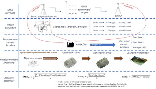
The methodology used in this work is shown in Figure 1.

Figure 1. Flowchart of the methodology used in this work.

2.1. Study site

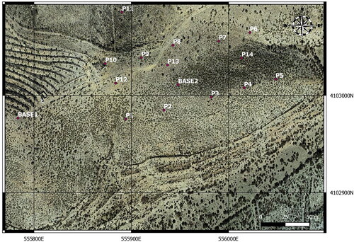
The study site is located in Tabernas, a small town in the province of Almeria (Spain). The south-west and north-east UTM coordinates (ETRS89 Zone 30) of this area are (555.770, 4.102.860) and (556.098, 4.103.095), respectively. So the area of the plot was 328 m by 235 m, covering 7.70 ha. Figure 2 shows the location of the study area.

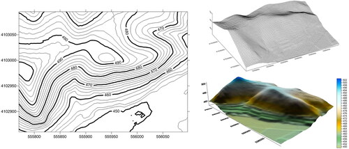
The choice of this area is based on its morphology and the proximity of a vertex of the REGENTE geodetic network (Red Geodésica Nacional por Técnicas Espaciales). The elevation range of the study area is 60 m, varying from 440 to 500 m above mean sea level (MSL). The vegetation in the area is of desert type, with no large trees and only small shrubs. Figure 3 shows the morphology of the study zone.

Figure 2. Location of the study area. Coordinates are referred to UTM Zone 30 N (European Terrestrial Reference System 1989, ETRS89).

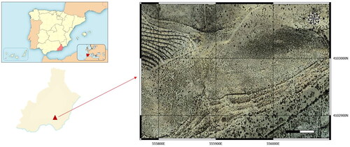
Figure 3. Morphology of the study zone.

2.2. GNSS surveying of ground Control points

Before the photogrammetric flights were performed, a traditional GNSS survey was carried out, materializing a total of 14 points distributed throughout the study site. All these points were materialized by means of targets that allowed their later viewing from the photographs taken by the UAV. The targets consisted of A3 size (420 mm by 297 mm) red paper on which was two black squares. Figure 4(b) shows a detail of one of these targets. The three-dimensional (3D) coordinates of these points were measured with a GNSS receiver working in RTK mode, with the fixed base station situated at the geodetic vertex of the REGENTE network called Bardinales, shown in Figure 4(a). The 3D coordinates of the base are 555783.214, 4102976.657 and 502.927 m, respectively. Horizontal coordinates are referred to UTM Zone 30 N (European Terrestrial Reference System 1989, ETRS89), and the elevation is referred to the MSL using the EGM08 REDNAP geoid model. Both rover and base GNSS receivers were Emlid Reach RS2 systems. For RTK measurements, these multi-band geodetic instruments have a manufacturer’s stated accuracy specification of ±7 mm +1 ppm horizontal RMS and ±14 mm +1 ppm vertical RMS. As the distance between the base station and the study area was approximately 200 m, the horizontal and vertical errors were around 7 and 14 mm. In addition, all targets were measured statically using a bipod by averaging all the observations received in the 60-second interval.

Figure 4. (a) Geodetic vertex of the REGENTE Network, named Bardinales; (b) Example of static target measurement for this work.

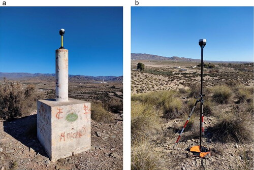
Once the topographic survey of the targets had been completed, the rover was restarted as a second fixed base station. Thus, prior to the start of the flights, two fixed base stations were available, Base 1 (located at the geodetic vertex of Bardinales) and Base 2, located in the central area of the study area. Figure 5 shows the final location status of the two bases and the 14 targets placed on the ground. The satellite constellation was always good, with PDOP (position dilution of precision) values below three in all flights.

Figure 5. Final disposition of the control targets used in this work and of the two fixed base stations.

2.3. Image acquisition

The images used in this work were taken from a rotatory wing DJI Phantom 4 RTK UAV with four rotors. This equipment has a navigation system using GPS and GLONASS. In addition, it is equipped with a front, rear and lower vision system that allows it to detect surfaces with a defined pattern and adequate lighting and avoid obstacles with a range between 0.2 and 7 m. The Phantom 4 RGB camera is equipped with a one-inch, 20-megapixel (5472 by 3648) sensor and has a manually adjustable aperture from F2.8 to F11. The lens has a fixed focal length of 8.8 mm and horizontal FOV of 84°. The technique of acquiring photographs from a UAV comes from airborne photogrammetry on the aircraft, in which a block of photographs is formed from parallel flight lines flown in a snake pattern at a stable altitude with a constant overlap and a vertical camera angle (90°) (Martin et al. 2016). The RTK system allows the storage of satellite observation data for PPK.

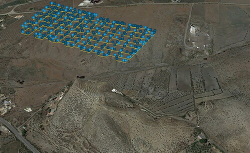
Three flights were performed at different altitudes: 50, 70 and 90 m, all measured from the take-off point located in the upper part of the study area. All flights were planned and executed automatically with DJI GS RTK application for the purpose of obtaining nadiral photographs. Also, all flights were performed with passes in two perpendicular directions in order to produce a full double grid. The 50-m flight consisted of a total of 366 photographs, with an equivalent mean GSD of 2.16 cm, arranged in seven longitudinal and 14 transverse passes. The flight at 70-m altitude consisted of a total of 195 photographs, with an equivalent mean GSD of 2.84 cm, arranged in four longitudinal and 10 transverse passes. The flight at 90-m altitude consisted of a total of 127 photographs, with an equivalent mean GSD of 3.48 cm, arranged in four longitudinal and eight transverse passes. In accordance with the flight altitude, the UAV speed and the light conditions at the time of flight, the shutter speed was adjusted to minimize the effect of blurring on the images taken. The camera was triggered every two seconds, and the flight speed was set to obtain forward and side overlaps of 70%. Figure 6 shows an example of the route followed by the drone for the flight at a 50-m altitude.

Figure 6. Example of the route followed by the drone for the 50-m height flight.

2.4. Post-processed camera locations

Once the three photogrammetric flights were completed, the observation data stored in the two GNSS fixed base stations (Base 1 and Base 2) were downloaded. The first step consisted of converting these observation files to Receiver Independent Exchange Format (RINEX) data using Emlid Studio software. In this way, we obtain from the .ubx file extension the navigation and observations files of the bases in .22 P and .22 O extensions, respectively. The next step consisted of applying the differential corrections of the bases to all the photographs obtained in the photogrammetric flight. This process was carried out using ATygeo version 1.8 software, which allows the correction of the photograph metadata from the drone navigation file (.obs) and the fixed base station observation and navigation files. This process was carried out twice, the first time from Base 1 and the second time from Base 2. Once the corrected metadata file was obtained from both bases, a third correction was made by averaging the corrections obtained at Bases 1 and 2. In this way, for each flight altitude, three sets of photographs with corrected metadata were obtained: Base 1, Base 2 and Average B1 and B2.

2.5. Photogrammetric processing

The photogrammetric process was carried out using the software package Agisoft Metashape Professional^© version 1.6.1.10009. This software is based on the SfM algorithm, and it obtains excellent results compared with other similar software (Sona et al. 2014; Zeybek and Serkan 2021). The photogrammetric processing consists of three main steps. First, the alignment of the images is carried out by feature identification and feature matching. Simultaneously, the software obtains internal and external camera orientation parameters, including non-linear radial distortion parameters. For this, the software only needs to start from an approximate focal length value, which is extracted from the EXIF metadata of the photographs. Different types of precision can be set, though in this work, it was set to medium. At the end of this step, the positions of each of the cameras, their orientation in space, the 3D coordinates of a sparse point cloud of the terrain and an estimation of the camera calibration parameters are obtained. The second step consists of referencing the sparse point cloud to an absolute coordinate system (ETRS89 and frames in the UTM, in the case of this study) and densifying it to obtain a much more defined model. This process was also executed with the quality of medium. Using the height field method, the mesh is obtained from the dense point cloud. The third step applies a texture to the mesh obtained in the previous step. Finally, the orthophoto is exported, and a grid DSM can be generated from the point cloud. As the geolocation data of the photographs has been obtained with high accuracy due to the GNSS RTK on board the drone, the bundle adjustment can be carried out without the use of GCPs, i.e. by direct georeferencing. However, all studies performed with conventional GNSS suggest that increasing the number of GCPs used during the camera calibration process for indirect georeferencing allows optimal accuracies to be obtained (Martínez-Carricondo et al. 2018; Sanz-Ablanedo et al. 2018). Therefore, the 14 field targets could be used interchangeably as GCPs or as CPs to evaluate the accuracy of the photogrammetric project. Under this approach, a total of 54 photogrammetric projects were processed according to the combinations shown in Table 1 and taking into account that for each possible combination, five repetitions were performed (GCPs from one to five). Thus, 234 results were obtained.

Table 1. Summary of photogrammetric projects carried out.

Flying height (m)	Fixed base station	Number of GCPs used	Repetitions
50	Base 1	0	–
70	Base 2	1	5
90	Average B1 and B2	2	5
–	–	3	5
–	–	4	5
–	–	5	5

2.6. Accuracy assessment

The accuracy of all photogrammetric projects was evaluated using the surveyed points that had not been used for georeferencing (CPs), using the typical root mean square error (RMSE) formulation (Martínez-Carricondo et al. 2018). From this formulation, RMSE_X, RMSE_Y and RMSE_Z were obtained, and finally, RMSE_T, which is the total error obtained in the CP.

3. Results

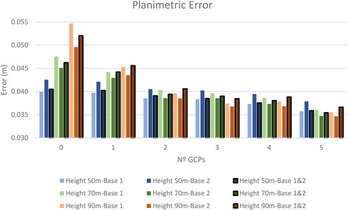
Figure 7 shows the results obtained for the planimetric error of the photogrammetric projects. For each flight height and for each correction base, from one GCP the graph shows the average value of the five repetitions carried out. For the 50-m height and corrections from Base 1, the error varied from 0.040 m without GCPs to 0.036 m with five GCPs. For the 50-m height and corrections from Base 2, the error ranged from 0.043 m without GCPs to 0.038 m with five GCPs. For the 50-m height and using both correction bases, the error ranged from 0.040 m without GCPs to 0.036 m with five GCPs. For the 70-m height and corrections from Base 1, the error ranged from 0.048 m without GCPs to 0.036 m with five GCPs. For the 70-m height and corrections from Base 2, the error ranged from 0.045 m without GCPs to 0.035 m with five GCPs. For the 70-m height and using both correction bases, the error ranged from 0.046 m without GCPs to 0.035 m with five GCPs. For the 90-m height and corrections from Base 1, the error ranged from 0.055 m without GCPs to 0.036 m with five GCPs. For the 90-m height and corrections from Base 2, the error ranged from 0.050 m without GCPs to 0.035 m with five GCPs. For the 90-m height and using both correction bases, the error ranged from 0.052 m without GCPs to 0.037 m with five GCPs.

Figure 7. Planimetric error obtained in photogrammetric projects.

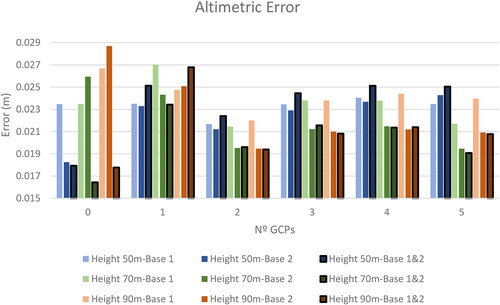
Figure 8 shows the results obtained for the altimetric error of the photogrammetric projects. For each flight height and for each correction base from one GCP onwards, the graph shows the average value of the five repetitions carried out. For the 50-m height and corrections from Base 1, the error had a fairly continuous behaviour, from 0.023 m without GCPs and reaching a maximum of 0.024 m for four GCPs. For the 50-m height and corrections from Base 2, the minimum error was 0.018 m without GCPs, and there was a maximum of 0.024 m for five GCPs. For the 50-m height and making use of the two correction bases, the minimum error was 0.018 m without GCPs, and the maximum was 0.025 m with four GCPs. For the 70-m height and corrections from Base 1, the error was 0.023 m without GCPs and a peak at 0.027 m with one GCP. For the 70-m height and corrections from Base 2, an error of 0.026 m was obtained without GCPs, and it decreased to 0.019 m with five GCPs. For the 70-m height and using both correction bases, the minimum error was 0.016 m without GCPs, and the maximum error was 0.023 m with one GCP. For the 90-m height and corrections from Base 1, the maximum error was 0.027 m without GCPs, and the minimum was 0.022 m for two GCPs. For the 90-m height and corrections from Base 2, the maximum error was 0.029 m without GCPs, and the minimum was 0.019 m for two GCPs. For the 90-m height and making use of the two correction bases, the minimum error was 0.018 m without GCPs, and the maximum was 0.027 m for one GCP.

Figure 8. Altimetric error obtained in photogrammetric projects.

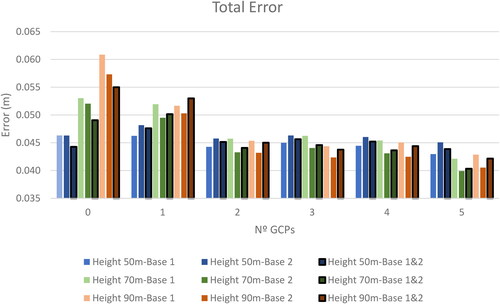
Figure 9 shows the composition of the total error obtained in the photogrammetric projects. For each flight height and for each correction base from one GCP onwards, the graph shows the average value of the five repetitions carried out. For the 50-m height and corrections from Base 1, the error ranges from 0.046 m without GCPs to 0.043 m for five GCPs. For the 50-m height and corrections from Base 2, the error ranges from 0.046 m without GCPs to 0.045 m for five GCPs. For the 50-m height and using the two correction bases, an error of 0.044 m is obtained without GCPs, with a maximum of 0.048 m for one GCP. For the 70-m height and corrections from Base 1, the error ranges from 0.053 m without GCPs to 0.042 m for five GCPs. For the 70-m height and corrections from Base 2, the error ranges from 0.052 m without GCPs to 0.040 m for five GCPs. For the 70-m height and using the two correction bases, an error of 0.049 m is obtained without GCPs, with a maximum of 0.050 m for one GCP and a minimum of 0.040 m for five GCPs. For the 90-m height and corrections from Base 1, the error varies from 0.061 m without GCPs to 0.043 m for five GCPs. For the 90-m height and corrections from Base 2, the error varies from 0.057 m without GCPs to 0.041 m for five GCPs. For the 90-m height and making use of the two correction bases, the error obtains a maximum of 0.055 m without GCPs and a minimum of 0.042 m for five GCPs.

Figure 9. Total error obtained in photogrammetric projects.

4. Discussion

If we focus only on the planimetric error, there is a clear trend that indicates that the error decreases as we increase the number of GCPs used during the bundle adjustment. This behaviour is in line with many studies carried out with UAVs and conventional GNSS (Agüera-Vega et al. 2017; Martínez-Carricondo et al. 2018; Sanz-Ablanedo et al. 2018). It is also evident that increasing the flight height increases the planimetric errors obtained, which is also in line with numerous previous studies (Agüera-Vega et al. 2016; Quoc Long et al. 2020). However, this seems to be limited as the number of GCPs increases, with all projects obtaining very similar values in the 0.035–0.037 m range. All these results have obtained the expected accuracy of one to two GSD. It seems clear, then, that it is possible to reduce the planimetric error either by increasing the number of GCPs or by reducing the flight height without using GCPs. For the planimetric error, the GNSS fixed base station chosen for the photo metadata corrections does not seem to have any influence, nor does the fact of averaging the data from two different bases. The results achieved are better than those obtained by (Eker et al. 2021), who analysed different reference station bases and concluding that the best results were obtained with a short-baseline PPK method obtaining corrections from a GNSS base station.

Regarding the analysis of the altimetric error, the influence of increasing the number of GCPs used in the bundle adjustment is not so evident. For the three flight heights and using only a single correction base, the best results have been obtained with two GCPs, but then there is a slight deterioration as the number of GCPs continues to increase. The influence of flight height on the altimetric error is not so evident either, though as the number of GCPs is varied, the error fluctuates randomly without a clear pattern that would allow conclusions to be drawn. This lack of a clear trend is consistent with the randomness of the results obtained by other authors (Ekaso et al. 2020; Forlani et al. 2018; Štroner et al. 2020; Taddia et al. 2020), even when duplicating flights with the same configuration and the same UAV. However, the best results have been obtained without using GCPs and by using metadata from the photographs averaged with the two correction bases. In fact, for these flights, when using a GCP, the results worsen significantly, though there is some improvement when increasing the GCPs. It is very interesting that for the three flight heights, the altimetric error without GCPs and with the two correction bases is clearly below the corresponding GSD, representing a great advance in terms of accuracy with respect to other previous studies, for example, the study by (Forlani et al. 2018). This is very enlightening, as it offers a different way to improve the accuracy of photogrammetric projects without the need to increase the number of GCPs as in (Canh et al. 2020; Losè et al. 2020; Taddia et al. 2020; Zhang et al. 2019) or to include oblique photographs to enhance camera calibration data as in the studies by (Losè et al. 2020; Štroner et al. 2021; Taddia et al. 2020; Vacca et al. 2017).

Regarding the total error, being the composition of the planimetric and altimetric error, there is still a clear pattern in which the flight height clearly influences the accuracy, especially when no GCPs are used. The classic pattern of improving accuracy as the number of GCPs increases is also maintained, but the influence of using two correction bases and flight height is no longer evident. The results are very similar from the use of two GCPs. However, for a flight height of 50 m and using the two correction bases, the increase in the number of GCPs produces a practically negligible improvement, obtaining an accuracy below two GSD and very similar to that obtained in other combinations with five GCPs.

5. Conclusions

UAVs equipped with GNSS RTK receivers allow direct georeferencing of the photogrammetric project without the need to use GCPs. The aim of this research has been to improve the accuracy of these photogrammetric projects without the need to use oblique photographs or GCPs. This research has demonstrated a complementary way to those explored by previous research, consisting of obtaining geolocation data from flight photographs as accurately as possible. To this end, the use of multiple GNSS fixed base stations has been proposed, correcting the geolocation data of the photographs simultaneously by averaging the differential corrections.

The results have shown how this methodology considerably reduces the altimetric errors, placing them in limits even below the GSD. Therefore, for flight altitudes of 50 m, improvements in altimetric accuracy of 14% were obtained, while for flight altitudes of 70 and 90 m the improvements in altimetric accuracy reached 35%. In relation to planimetric error, no significant improvements have been observed. However, the total errors are similar to those obtained with various combinations of GCPs and closed to the GSD of the photogrammetric project.

This advance represents a new methodology to obtain accurate UAV photogrammetry results in those cases where the use of GCPs is not feasible, gaining in operator safety and reducing operation times.

Author’s responsibilities

The contributions of the authors were: Conceptualization, P.M.-C., F.C.-R. and F.A.-V.; methodology, P.M.-C., F.C.-R. and F.A.-V.; software P.M.-C.; validation, P.M.-C.; formal analysis, P.M.-C., F.C.-R. and F.A.-V.; investigation, P.M.-C., F.C.-R. and F.A.-V.; resources, F.C.-R. and F.A.-V.; writing—original draft preparation, P.M.-C.; writing—review and editing, P.M.-C., F.C.-R. and F.A.-V.; visualization, P.M.-C.; project administration,P.M.-C. All authors have read and agreed to the published version of the manuscript.

Data availability statement

The data that support the findings of this study are openly available in “figshare” at 10.6084/m9.figshare.19509961 reference number.

Disclosure statement

No potential conflict of interest was reported by the authors.

Additional information

Funding

This work was supported by the Grant for Bridge Projects of the Plan for Research and Transfer 2021 of University of Almeria (PPUENTE2021/003).

References

- Aber JS, Marzolff I, Ries JB. 2010. Small-format aerial photography. Amsterdam, Netherlands: Elsevier.
- Agüera-Vega F, Carvajal-Ramírez F, Martínez-Carricondo P. 2016. Accuracy of digital surface models and orthophotos derived from unmanned aerial vehicle photogrammetry. J Surv Eng. 143:04016025.
- Agüera-Vega F, Carvajal-Ramírez F, Martínez-Carricondo P. 2017. Assessment of photogrammetric mapping accuracy based on variation ground control points number using unmanned aerial vehicle. Measurement. 98:221–227.
- Agüera-Vega F, Carvajal-Ramírez F, Martínez-Carricondo P, Sánchez-Hermosilla López J, Mesas-Carrascosa FJ, García-Ferrer A, Pérez-Porras FJ. 2018. Reconstruction of extreme topography from UAV structure from motion photogrammetry. Measurement. 121:127–138.
- Akar Ö. 2018. The rotation forest algorithm and object-based classification method for land use mapping through UAV images. Geocarto Int. 33(5):538–553.
- Blistan P, Jacko S, Kovanič Ľ, Kondela J, Pukanská K, Bartoš K. 2020. Tls and Sfm approach for bulk density determination of excavated heterogeneous raw materials. Minerals. 10(2):174.
- Brunier G, Michaud E, Fleury J, Anthony EJ, Morvan S, Gardel A. 2020. Assessing the relationship between macro-faunal burrowing activity and mudflat geomorphology from UAV-based structure-from-motion photogrammetry. Remote Sens Environ. 241:111717.
- Canh L, VAN C, Xuan Cuong N, Quoc Long L, Thi Thu Ha T, Trung Anh, X, Nam Bui. 2020. Experimental investigation on the performance of DJI phantom 4 RTK in the PPK mode for 3d mapping open-pit mines. Inz Miner. 1(1):65–74.
- Carvajal-Ramírez F, Navarro-Ortega AD, Agüera-Vega F, Martínez-Carricondo P, Mancini F. 2019. Virtual reconstruction of damaged archaeological sites based on unmanned aerial vehicle photogrammetry and 3D modelling. Study case of a Southeastern Iberia production area in the Bronze Age. Measurement. 136:225–236.
- Carvajal-Ramírez F, da Silva JRM, Agüera-Vega F, Martínez-Carricondo P, Serrano J, Jesús Moral F. 2019. Evaluation of fire severity indices based on pre- and post-fire multispectral imagery sensed from UAV. Remote Sens. 11:993.
- Cledat E, Jospin LV, Cucci DA, Skaloud J. 2020. Mapping quality prediction for RTK/PPK-equipped micro-drones operating in complex natural environment. ISPRS J Photogramm Remote Sens. 167:24–38.
- Doumit JA. 2019. Structure from motion technology for historic building information modeling of Toron fortress (Lebanon). In Proc. Int. Conf. InterCarto, InterGIS (vol. 25).
- Ekaso D, Nex F, Kerle N. 2020. Accuracy assessment of real-time kinematics (RTK) measurements on Unmanned Aerial Vehicles (UAV) for direct geo-referencing. Geo-Spatial Inform Sci. 23(2):165–181.
- Eker R, Alkan E, Aydın A. 2021. A comparative analysis of UAV-RTK and UAV-PPK methods in mapping different surface types. Eur J For Eng. 7(1):12–25.
- Elkhrachy I. 2021. Accuracy assessment of low-cost Unmanned Aerial Vehicle (UAV) photogrammetry. Alex Eng J. 60(6):5579–5590.
- Eltner A, Mulsow C, Maas HG. 2013. Quantitative measurement of soil erosion from tls and UAV data. Int Arch Photogramm Remote Sens Spatial Inform Sci. XL-1/W20:119–124.
- Famiglietti NA, Cecere G, Grasso C, Memmolo A, Vicari A. 2021. A test on the potential of a low cost unmanned aerial vehicle Rtk/Ppk solution for precision positioning. Sensors. 21(11):3882.
- Fernando P, Carvajal-Ram F, Mart P, Garc A. 2018. Drift correction of lightweight microbolometer thermal sensors on-board unmanned aerial vehicles. Remote Sens. 10:615.
- Ferrer-González E, Agüera-Vega F, Carvajal-Ramírez F, Martínez-Carricondo P. 2020. UAV photogrammetry accuracy assessment for corridor mapping based on the number and distribution of ground control points. Remote Sens. 12(15):2447.
- Forlani G, Diotri F, Morra Di Cella U, Roncella R. 2020. UAV block georeferencing and control by on-board GNSS data. Int Arch Photogramm Remote Sens Spatial Inform Sci. 43:9–16.
- Forlani G, Asta ED, Diotri F, Morra U, Roncella R, Santise M. 2018. Quality assessment of DSMs produced from UAV flights georeferenced with on-board RTK positioning. Remote Sens. 10:311.
- Gerke M, Nex F, Remondino F, Jacobsen K, Kremer J, Karel W, Huf H, Ostrowski W. 2016. Orientation of oblique airborne image sets - experiences from the ISPRS/Eurosdr benchmark on multi-platform photogrammetry. Int Arch Photogramm Remote Sens Spatial Inform Sci Arch. 2016
- Gerke M, Przybilla HJ. 2016. Accuracy analysis of photogrammetric UAV image blocks: influence of onboard RTK-GNSS and cross flight patterns. Photogrammetr Fernerkund Geoinform. 2016(1):1730.
- Grenzdörffer GJ, Engel A, Teichert B. 2008. The photogrammetric potential of low-cost UAVs in forestry and agriculture. Int Arch Photogramm Remote Sens Spatial Inform Sci. 31(B3):1207–1214.
- Hartling S, Sagan V, Maimaitijiang M. 2021. Urban tree species classification using UAV-based multi-sensor data fusion and machine learning. GIScience Remote Sens. 58(8):1250–1275.
- Huang CY, Wei HL, Rau JY, Jhan JP. 2019. Use of principal components of UAV-acquired narrow-band multispectral imagery to map the diverse low stature cegetation FAPAR. GIScience Remote Sens. 56(4):605–623.
- Hugenholtz C, Brown O, Walker J, Barchyn T, Nesbit P, Kucharczyk M, Myshak S. 2016. Spatial accuracy of UAV-derived orthoimagery and topography: comparing photogrammetric models processed with direct geo-referencing and ground control points. Geomatica. 70:21–30.
- Jaud M, Passot S, Bivic RL, Delacourt C, Grandjean P, Dantec NL. 2016. Assessing the accuracy of high resolution digital surface models computed by PhotoScan® and MicMac® in sub-optimal survey conditions. Remote Sens. 8(6):465.
- Jon J, Koska B, Pospíšil J. 2013. Autonomous airship equipped by multi-sensor mapping platform. Int Arch Photogramm Remote Sens Spatial Inform Sci. 40:119–124.
- Kamal WA, Samar R. 2008. A mission planning approach for UAV applications. Proceedings of the IEEE Conference on Decision and Control. p. 3101–3106.
- Kanistras K, Martins G, Rutherford MJ, Valavanis KP. 2015. Survey of unmanned aerial vehicles (UAVS) for traffic monitoring. Handbook of unmanned aerial vehicles. Dordrecht, Netherlands: Springer Netherlands.
- Koska B, Křemen T. 2013. The combination of laser scanning and structure from motion technology for creation of accurate exterior and interior orthophotos of st. Nicholas Baroque church. Int Arch Photogramm Remote Sens Spatial Inform Sci. XL-5/W1:133–138.
- Křemen T. 2019. Measurement and documentation of St. Spirit church in liběchov. Advances and Trends in Geodesy, Cartography and Geoinformatics II - Proceedings of the 11th International Scientific and Technical Conference on Geodesy, Cartography and Geoinformatics, GCG 2019.
- Kršák B, Blišťan P, Pauliková A, Puškárová P, Kovanič L, Palková J, Zelizňaková V. 2016. Use of low-cost UAV photogrammetry to analyze the accuracy of a digital elevation model in a case study. Measur J Int Measur Confed. 91:276–287.
- Liu PAY, Chen YN, Huang JY, Han JS, Lai SC, Kang TH, Wu MC, Wen Meng-Han Tsai. 2014. A review of rotorcraft Unmanned Aerial Vehicle (UAV) developments and applications in civil engineering. Smart Struct Syst. 13(6):1065–1094.
- Losè L, Teppati F, Chiabrando, F, Giulio Tonolo. 2020. Boosting the timeliness of UAV large scale mapping. Direct georeferencing approaches: operational strategies and best practices. ISPRS Int J Geo-Inform. 9(10):578.
- Martin RA, Rojas I, Franke K, Hedengren JD. 2016. Evolutionary view planning for optimized UAV terrain modeling in a simulated environment. Remote Sens. 8:26.
- Martínez-Carricondo P, Francisco Agüera-Vega Fernando Carvajal-Ramírez FJ, Mesas-Carrascosa A, García-Ferrer, FJ, Pérez-Porras. 2018. Assessment of UAV-photogrammetric mapping accuracy based on variation of ground control points. Int J Appl Earth Observ Geoinform. 72:1–10.
- Martínez-Carricondo P, Carvajal-Ramírez F, Yero-Paneque L, Agüera-Vega F. 2019. Combination of nadiral and oblique UAV photogrammetry and HBIM for the virtual reconstruction of cultural heritage. Case study of Cortijo Del Fraile in Níjar, Almería (Spain). Build Res Inform. 48(2):140–159.
- Meinen BU, Robinson DT. 2020. Mapping erosion and deposition in an agricultural landscape: optimization of UAV image acquisition schemes for SfM-MVS. Remote Sens Environ. 239:111666.
- Mirjam Bilker H, Eija, J, Juha. 1998. GPS supported aerial triangulation using untargeted ground control. Int Arch Photogramm Remote Sens. 32.
- Navarro A, Young M, Allan B, Carnell P, Macreadie P, Ierodiaconou D. 2020. The application of unmanned aerial vehicles (UAVs) to estimate above-ground biomass of mangrove ecosystems. Remote Sens Environ. 242:111747.
- Nesbit PR, Hugenholtz CH. 2019. Enhancing UAV-SfM 3D model accuracy in high-relief landscapes by incorporating oblique images. Remote Sens. 11(3):239.
- Padró JC, Javier Muñoz F, Planas J, Pons X. 2019. Comparison of four UAV georeferencing methods for environmental monitoring purposes focusing on the combined use with airborne and satellite remote sensing platforms. Int J Appl Earth Observ Geoinform. 75:130–140.
- Park S, Choi Y. 2020. Applications of unmanned aerial vehicles in mining from exploration to reclamation: a review. Minerals. 10(8):663.
- Pavlidis G, Koutsoudis A, Arnaoutoglou F, Tsioukas V, Chamzas C. 2007. Methods for 3D digitization of cultural heritage. J Cult Heritage. 8(1):93–98.
- Peppa MV, Hall J, Goodyear J, Mills JP. 2019. Photogrammetric assessment and comparison of Dji phantom 4 pro and phantom 4 Rtk small unmanned aircraft systems. Int Arch Photogramm Remote Sens Spatial Inform Sci. 42:503–509.
- Pérez JA, Gonçalves GR, Charro MC. 2019. On the positional accuracy and maximum allowable scale of UAV-derived photogrammetric products for archaeological site documentation. Geocarto Int. 34(6):575–585.
- Piras M, Taddia G, Forno MG, Gattiglio M, Aicardi I, Dabove P, Russo SL, Lingua A. 2017. Detailed geological mapping in mountain areas using an unmanned aerial vehicle: application to the Rodoretto Valley, NW Italian Alps. Geomatics Nat Hazards Risk. 8:137–149.
- Puliti S, Theodor Ene L, Gobakken T, Næsset E. 2017. Use of partial-coverage UAV data in sampling for large scale forest inventories. Remote Sens Environ. 194:115–126.
- Püschel H, Sauerbier M, Eisenbeiss H. 2008. A 3D model of castle landenberg (CH) from combined photogrametric processing of terrestrial and UAV based images. Int Arch Photogramm Remote Sens. Spat Inf Sci.
- Quoc Long N, Goyal R, Khac Luyen B, VAN Canh L, Xuan Cuong C, VAN Chung P, Ngoc Quy B, Bui XN. 2020. Influence of flight height on the accuracy of UAV derived digital elevation model at complex terrain. Inż Miner. 45:179–187.
- Salvo G, Caruso L, Scordo A. 2014. Urban traffic analysis through an UAV. Proc Soc Behav Sci. 111:1083–1091.
- Sankey JB, Temuulen T, Sankey J, Li S, Ravi G, Wang J, Caster, A, Kasprak. 2021. Quantifying plant-soil-nutrient dynamics in rangelands: fusion of UAV hyperspectral-LiDAR, UAV multispectral-photogrammetry, and ground-based LiDAR-digital photography in a shrub-encroached desert grassland. Remote Sens Environ. 253:112223.
- Santise M, Fornari M, Forlani G, Roncella R. 2014. Evaluation of dem generation accuracy from UAS imagery. Int Arch Photogramm Remote Sens Spatial Inform Sci. 40:333–337.
- Sanz-Ablanedo Enoc Jim Chandler J, Rodríguez-Pérez C, Ordóñez Enoc Sanz-Ablanedo, JH, Chandler, Rodríguez-Pérez JR, Ordóñez C. 2018. Accuracy of Unmanned Aerial Vehicle (UAV) and SfM photogrammetry survey as a function of the number and location of ground control points used. Remote Sens. 10(10):1606.
- Snavely N, Seitz SM, Szeliski R. 2008. Modeling the world from internet photo collections. Int J Comput Vis. 80(2):189–210.
- Sona G, Pinto L, Pagliari D, Passoni D, Gini R. 2014. Experimental analysis of different software packages for orientation and digital surface modelling from UAV images. Earth Sci Inform. 7(2):97–107.
- Stefanik K, Gassaway J, Kochersberger K, Abbott A. 2011. UAV-based stereo vision for rapid aerial terrain mapping. GIScience Remote Sens. 48(1):24–49.
- Štroner M, Urban R, Reindl T, Jan S, Josef B. 2020. Evaluation of the georeferencing accuracy of a photogrammetric model using a quadrocopter with onboard GNSS RTK. Sensors (Switzerland). 20(8):2318.
- Štroner M, Urban R, Seidl J, Reindl T, Brouček J. 2021. Photogrammetry using UAV-mounted GNSS RTK: georeferencing strategies without GCPs. Remote Sensing. 13(7):1336.
- Taddia Y, Stecchi F, Pellegrinelli A. 2020. Coastal mapping using dji phantom 4 RTK in post-processing kinematic mode. Drones. 4(2):9.
- Tahar KN, Kamarudin SS. 2016. UAV onboard GPS in positioning determination. Int Arch Photogramm Remote Sens Spatial Inform Sci. XLI-B1.
- Themistocleous K, Agapiou A, Hadjimitsis D. 2016. 3D documentation and BIM modeling of cultural heritage structures using UAVS: the case of the Foinikaria Church. Int Arch Photogramm Remote Sens Spatial Inform Sci. XLII-2/W:45–49.
- Tian J, Wang L, Li X, Gong H, Shi C, Zhong R, Liu X. 2017. Comparison of UAV and WorldView-2 imagery for mapping leaf area index of mangrove forest. Int J Appl Earth Observ Geoinform. 61:22–31.
- Tomaštík J, Mokroš M, Surový P, Grznárová A, Merganič J. 2019. UAV RTK/PPK method-an optimal solution for mapping inaccessible forested areas? Remote Sens. 11(6):721.
- Türk T, Tunalioglu N, Erdogan B, Ocalan T, Gurturk M. 2022. Accuracy assessment of UAV-post-processing kinematic (PPK) and UAV-traditional (with ground control points) georeferencing methods. Environ Monitor Assess. 194(7):476.
- Urban R, Štroner M, Kuric I. 2020. The use of onboard UAV Gnss navigation data for area and volume calculation. Acta Mont Slovac. 25(3):361–374.
- Vacca G, Dessì A, Sacco A. 2017. The use of nadir and oblique UAV images for building knowledge. ISPRS Int J Geo-Inform. 6(12):393.
- Varbla S, Puust R, Ellmann A. 2020. Accuracy assessment of RTK-GNSS equipped UAV conducted as-built surveys for construction site modelling. Survey Rev. 53:477–492.
- Vasuki Y, Holden EJ, Kovesi P, Micklethwaite S. 2014. Semi-automatic mapping of geological structures using UAV-based photogrammetric data: an image analysis approach. Comput Geosci. 69:22–32.
- Yao H, Qin R, Chen X. 2019. Unmanned aerial vehicle for remote sensing applications - a review. Remote Sens. 11:1443.
- Yuan C, Zhang Y, Liu Z. 2015. A survey on technologies for automatic forest fire monitoring, detection, and fighting using unmanned aerial vehicles and remote sensing techniques. Can J For Res. 45:150312143318009.
- Žabota B, Kobal M. 2021. Accuracy assessment of UAV-photogrammetric-derived products using PPK and GCPS in challenging terrains: in search of optimized rockfall mapping. Remote Sens. 13(19):3812.
- Zeybek M. 2021. Accuracy assessment of direct georeferencing UAV images with onboard global navigation satellite system and comparison of CORS/RTK surveying methods. Meas Sci Technol. 32(6):065402.
- Zeybek M, Serkan B. 2021. 3D dense reconstruction of road surface from UAV images and comparison of SfM based software performance. Turk J Remote Sens GIS.
- Zhang H, Aldana-Jague E, Clapuyt F, Wilken F, Vanacker V, Van Oost K. 2019. Evaluating the potential of post-processing kinematic (PPK) georeferencing for UAV-based structure-from-motion (SfM) photogrammetry and surface change detection. Earth Surf Dyn. 7(3):807–827.