Multidecadal evaluation of changes in coffee-growing areas using Landsat data in Central Highlands, Vietnam

Abstract

Vietnam is the world’s second-largest coffee exporter. Information on coffee-growing areas is thus important for production estimation. This research developed an approach for coffee mapping and change detection using Landsat and DEM data in Central Highlands, Vietnam. The data were processed for 1995, 2005, and 2020 using random forests (RF). The mapping results, verified with reference data, showed overall accuracy and Kappa coefficient higher than 86.9% and 0.74, respectively. These findings were reaffirmed by a close relationship between the satellite-based coffee area and official statistics, with the root mean squared percentage error (RMSPE) and mean absolute percentage error (MAPE) greater than 9.9% and 7.6%, respectively. From 1995 to 2020, the newly planted coffee area increased by 135,520 ha, due to the conversion of forests to coffee plantations. Such distributions of coffee areas and decadal changes in farming activities are critically useful for policymakers to formulate successful crop planning strategies.

Keywords:

• Landsat data
• random forests
• coffee
• change detection
• Vietnam

1. Introduction

Coffee is one of the world’s most traded agricultural commodities and popular beverages, consumed by at least one-third of the world’s population. It is among the most valuable tropical export crops, cultivated on an estimated area of roughly 10.9 million hectares across more than 80 countries (Statista 2019), with approximately 125 million people relying on it for their economic survival (Krishnan 2017). Vietnam is globally the second largest coffee exporter after Brazil (Adriana 2019; ICO 2020; Santos et al. 2021), annually producing roughly 1763,500 tones (GSO 2020). Coffee is the country’s second most valuable agricultural export after rice, playing considerable socioeconomic importance in the country because it provides income sources and rural livelihoods for at least two million people living in the Central Highlands. Dak Lak is the home of robusta coffee, and the largest coffee-producing province in Vietnam, contributing approximately 31.8% and 27.1% of the nation’s total coffee-growing area and production, respectively (DLSO 2020; GSO 2020). Most of the region’s coffee is produced by smallholder farmers using intensive farming methods.

Driven by the rapidly growing population from 1.5 million people in 2000 to 2.1 million people in 2019, coupled with favorable coffee prices on the world market and advantages of land suitability for coffee production in the study region, the area allocated for coffee production had significantly increased from 7,000 ha in 1975 to about 209,955 ha in 2020 (Kim and Hoang 2013; GSO 2020). The expansion of coffee-growing areas has resulted in a steady decline in the forest cover in the province, especially in areas where basaltic soils are suitable for establishing large-scale coffee plantations. During the movement, coffee remained the primary income source in the region, contributing more than 40% of the provincial gross domestic product (Cairns 2017). However, in recent years, coffee growers in the region have faced increasing challenges, including fluctuating coffee prices, extreme weather events, and land degradation due to intensitive cultivation, threatening coffee production and farmers’ livelihoods. For example, the occurrence of severe droughts in 2016 has resulted in a 20−90% reduction in water discharges from major rivers, affecting approximately 170,000 ha of cropping areas across the province (CGIAR 2016).

Because the province has encountered coffee intensification issues and environmental impacts, a decadal understanding of changes in the coffee landscape from temporal and spatial perspectives is important to give valuable insights into crop management and agricultural planning processes. Remote sensing is widely recognized as an important tool for agricultural planning because it can provide spatial and temporal datasets, which are essential for land-use/land-cover (LULC) assessment and modelling. Nevertheless, there have been few remote sensing studies on the classification and monitoring changes in coffee-planted areas in the country’s Central Highlands (Müller 2002; Meyfroidt et al. 2013; Le et al. 2022; Thao et al. 2022). In this work, Landsat data and digital elevation model (DEM) were used for mapping and analysis of multidecadal changes of coffee cultivated areas in the region. The utilization of Landsat images for LULC monitoring studies has gained interest among agronomists and researchers around the world, because of the wide spatial coverage and free historical archives of satellite data. Many scientists successfully used multi-temporal Landsat imageries for coffee mapping and change analysis (Cordero‐Sancho and Sader 2007; Ortega-Huerta et al. 2012; Schmitt-Harsh et al. 2013; Kawakubo and Machado 2016; Chemura et al. 2017a; 2017b; Hunt et al. 2020). Furthermore, several studies have incorporated DEM data into the processes of satellite image classification and demonstrated to improve the overall accuracy of LULC classification (Eiumnoh and Shrestha 2000; Dorren et al. 2003; Qi et al. 2009; Yin et al. 2022).

Among algorithms recently developed for image classification and regression analysis, the random forests (RF) (Breiman et al. 1984; Breiman 2001) has been extensively exploited due to its great performance on many issues, and yield reliable results, particularly when dealing with complex and non-linear datasets (Rodriguez-Galiano et al. 2012; Son et al. 2017; Saini and Ghosh 2018; Peng et al. 2019; Mansaray et al. 2020). Furthermore, this method can also be used to choose and rank independent variables with the greatest ability for regression analysis and classification between targets, which is important to reduce the computational cost and error-prone, when processing high-dimensional satellite datasets (Körting et al. 2013; Belgiu and Dragut 2016; Speiser 2021). The RF likely produces more accurate prediction results than other methods, such as decision trees, support vector machines (SVM), artificial neural networks (ANN), and recurrent neural networks (RNN) due to its less prone to overfitting problems (Caruana and Niculescu-Mizil 2006; Caruana et al. 2008; Miller et al. 2019; Martinez‐Castillo et al. 2020; Ali 2021; Tan et al. 2021). It also produces competitive results with time-consuming deep-learning neural networks in different mapping applications using remotely sensed data (Mboga et al. 2017; Wright and Ziegler 2017; Shiferaw et al. 2019; Ge et al. 2020; Sheykhmousa et al. 2020; Velásquez et al. 2020; Mohajane et al. 2021; Velásquez et al. 2021). Other advantages of RF include easily implementing and computing acceleration in a parallel structure for a large geospatial dataset, handling numerous and complex input variables, being vigorous to noise and outliers, mitigating data variance without increasing prediction bias, and creating more generalized solutions (Belgiu and Dragut 2016; Miller et al. 2019; Jain et al. 2020; Lawson et al. 2021; Lu 2021).

In this work, rather than comparing classification accuracies among methods, our ultimate goal was to map coffee-growing areas and accordingly delineate changes in coffee farming activities in the Central Highlands of Vietnam during periods 1995−2005 and 2005−2020 using the RF algorithm. The findings obtained from this work in the form of quantitative information on spatiotemporal distributions and decadal changes in coffee-growing areas could be beneficial to land-use planners and policymakers to formulate successful crop management and agricultural planning strategies in the province.

2. Study area and data collection

The study region (Dak Lak province), which was dissolved from Dak Lak and Dak Nong provinces in 2004, is situated in the Central Highlands of Vietnam, encompassing roughly 13,030.5 km² and lying between 12°40’N 108°3’E (Figure 1). This province was home to approximately 2.1 million people in 2019 with a density of 160 people/km², in which more than 70% of the population was living in rural areas and relying on agriculture for their livelihoods. The region is blessed with vast natural resources, mainly well-drained basaltic soils that are suitable for the cultivation of industrial trees, especially coffee, cashew, rubber, and pepper. The climate is tropical with two distinct seasons. The wet season lasts from May to November, and the dry season is from December to April. The annual precipitation ranges between 1,500 to 2,400 mm, with more than 80% of the total precipitation occurring during the rainy season. The air temperature is between 20–25 °C, with the highest temperatures of 27–31 °C in April and May. Dak Lak is the largest coffee-producing province in Vietnam, playing a crucial important role in the country’s economy of the Central Highlands. Coffee production in the province is typically practiced from October of the previous year to September, and harvested by the end of October to January (Table 1).

Figure 1. Map of the study region concerning elevation levels, administrative boundaries of districts, and national geography of Vietnam.

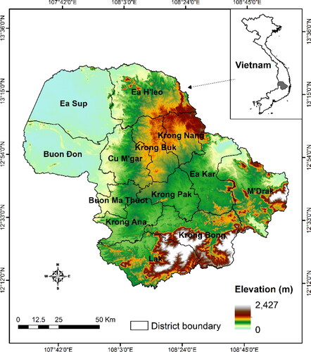
Table 1. Vegetation indices calculated from Landsat data.

No.	Index	Acronym	Expression	Reference
1	Ashburn vegetation index reflectance index	ARI	$2\times {\rho }_{\mathit{nir}}-{\rho }_{\mathit{red}}$	(Ashburn 1978)
2	Atmospherically resistant vegetation index	ARVI	$\frac{{\rho }_{\mathit{nir}}-[{\rho }_{\mathit{red}}-({\rho }_{\mathit{blue}}-{\rho }_{\mathit{red}})]}{{\rho }_{\mathit{nir}}+[{\rho }_{\mathit{red}}-({\rho }_{\mathit{blue}}-{\rho }_{\mathit{red}})]}$	(Kaufman and Tanre 1992)
3	Atmospherically resistant vegetation index 2	ARVI2	$-0.18+1.17\times \frac{{\rho }_{\mathit{nir}}+{\rho }_{\mathit{red}}}{{\rho }_{\mathit{nir}}+{\rho }_{\mathit{red}}}$	(Kaufman and Tanre 1992)
4	Adjusted transformed soil-adjusted vegetation index	ATSAVI	$\frac{a\times ({\rho }_{\mathit{nir}}-a\times {\rho }_{\mathit{red}}-b)}{a\times {\rho }_{\mathit{nir}}+{\rho }_{\mathit{red}}-a\times b+X(1+a^2)}$ a = 1.22, b = 0.03, X = 0.08	(Baret and Guyot 1991)
5	Blue-normalized difference vegetation index	BNDVI	$\frac{{\rho }_{\mathit{nir}}-{\rho }_{\mathit{blue}}}{{\rho }_{\mathit{nir}}+{\rho }_{\mathit{blue}}}$	(Yang et al. 2007)
6	Blue-wide dynamic range vegetation index	BWDRVI	$\frac{0.1\times {\rho }_{\mathit{nir}}-{\rho }_{\mathit{blue}}}{0.1\times {\rho }_{\mathit{nir}}+{\rho }_{\mathit{blue}}}$	(Hancock and Dougherty 2007)
7	Chlorophyll vegetation index	CVI	$\frac{{\rho }_{\mathit{nir}}\times {\rho }_{\mathit{red}}}{{({\rho }_{\mathit{green}})}^2}$	(Hunt et al. 2011)
8	Difference vegetation index	DVI	$2.4\times ({\rho }_{\mathit{nir}}-{\rho }_{\mathit{red}})$	(Richardsons and Wiegand 1977)
9	Enhanced vegetation index	EVI	$\frac{2.5\times ({\rho }_{\mathit{nir}}-{\rho }_{\mathit{red}})}{{\rho }_{\mathit{nir}}+6\times {\rho }_{\mathit{red}}-7.5\times {\rho }_{\mathit{blue}}+1}$	(Huete et al. 2002)
10	Enhanced vegetation index 2	EVI2	$\frac{2.4\times ({\rho }_{\mathit{nir}}-{\rho }_{\mathit{red}})}{{\rho }_{\mathit{nir}}+{\rho }_{\mathit{red}}+1}$	(Jiang et al. 2008)
11	Green atmospherically resistant vegetation index	GARI	$\frac{{\rho }_{\mathit{nir}}-[{\rho }_{\mathit{green}}-({\rho }_{\mathit{blue}}-{\rho }_{\mathit{red}})]}{{\rho }_{\mathit{nir}}-[{\rho }_{\mathit{green}}+({\rho }_{\mathit{blue}}-{\rho }_{\mathit{red}})]}$	(Gitelson et al. 1996)
12	Green-blue normalized difference vegetation index	GBNDVI	$\frac{{\rho }_{\mathit{nir}}-({\rho }_{\mathit{green}}-{\rho }_{\mathit{blue}})}{{\rho }_{\mathit{nir}}+({\rho }_{\mathit{green}}-{\rho }_{\mathit{blue}})}$	(Tucker et al. 1979)
13	Green chlorophyll index	GCI	$\frac{{\rho }_{\mathit{nir}}}{{\rho }_{\mathit{green}}}-1$	(Gitelson et al. 2003)
14	Green difference vegetation index	GDVI	${\rho }_{\mathit{nir}}-{\rho }_{\mathit{green}}$	(Tucker et al. 1979)
15	Global environmental monitoring index	GEMI	$n\times (1-0.25\times n)-\frac{{\rho }_{\mathit{red}}-0.125}{1-{\rho }_{\mathit{red}}}$ $n=\frac{2\times [{({\rho }_{\mathit{nir}})}^2-{({\rho }_{\mathit{red}})}^2+1.5\times {\rho }_{\mathit{nir}}+0.4\times {\rho }_{\mathit{red}}}{{\rho }_{\mathit{nir}}+{\rho }_{\mathit{red}}+0.5}$	(Pinty and Verstraete 1992)
16	Green leaf index	GLI	$\frac{2\times {\rho }_{\mathit{green}}-{\rho }_{\mathit{red}}-{\rho }_{\mathit{blue}}}{2\times {\rho }_{\mathit{green}}+{\rho }_{\mathit{red}}+{\rho }_{\mathit{blue}}}$	(Gobron et al. 2000)
17	Green normalized difference vegetation index	GNDVI	$\frac{{\rho }_{\mathit{nir}}-{\rho }_{\mathit{green}}}{{\rho }_{\mathit{nir}}+{\rho }_{\mathit{green}}}$	(Gitelson et al. 1996)
18	Green optimized soil-adjusted vegetation index	GOSAVI	$\frac{{\rho }_{\mathit{nir}}-{\rho }_{\mathit{green}}}{{\rho }_{\mathit{nir}}+{\rho }_{\mathit{green}}+0.16}$	(Rondeaux et al. 1996)
19	Green-red normalized difference vegetation index	GRNDVI	$\frac{{\rho }_{\mathit{nir}}-({\rho }_{\mathit{green}}+{\rho }_{\mathit{red}})}{{\rho }_{\mathit{nir}}+({\rho }_{\mathit{green}}+{\rho }_{\mathit{red}})}$	(Wang et al. 2007)
20	Global vegetation moisture index	GVMI	$\frac{({\rho }_{\mathit{nir}}+0.1)-({\rho }_{\mathit{swir}2}+0.02)}{({\rho }_{\mathit{nir}}+0.1)+({\rho }_{\mathit{swir}2}+0.02)}$	(Glenn et al. 2010)
21	Normalized difference vegetation index	NDVI	$\frac{{\rho }_{\mathit{nir}}-{\rho }_{\mathit{red}}}{{\rho }_{\mathit{nir}}+{\rho }_{\mathit{red}}}$	(Tucker 1979)
22	Infrared percentage vegetation index	IPVI	$0.5\times \left(\frac{{\rho }_{\mathit{nir}}}{{\rho }_{\mathit{nir}}+{\rho }_{\mathit{red}}}\right)\times (\mathit{NDVI}+1)$	(Crippen 1990)
23	Modified non-linear index	MNLI	$\frac{\left[{({\rho }_{\mathit{nir}})}^2-{\rho }_{\mathit{red}}\right]\times (1+0.5)}{{({\rho }_{\mathit{nir}})}^2-{\rho }_{\mathit{red}}-0.5}$	(Yang et al. 2008)
24	Modified soil-adjusted vegetation index	MSAVI	$\frac{2\times {\rho }_{\mathit{nir}}+1-\sqrt{{(2\times {\rho }_{\mathit{nir}}+1)}^2-8\times ({\rho }_{\mathit{nir}}-{\rho }_{\mathit{red}})}}{2}$	(Qi et al. 1994)
25	Modified triangular vegetation index 2	MTVI2	$1.5\times \frac{1.2\times ({\rho }_{\mathit{nir}}-{\rho }_{\mathit{green}})-2.5\times ({\rho }_{\mathit{red}}-{\rho }_{\mathit{green}})}{\sqrt{{(2\times {\rho }_{\mathit{nir}}+1)}^2-(6\times {\rho }_{\mathit{nir}}-5\times \sqrt{{\rho }_{\mathit{red}}})-0.5}}$	(Haboudane et al. 2004)
26	Normalized difference water index	NDWI	$\frac{{\rho }_{\mathit{green}}-{\rho }_{\mathit{nir}}}{{\rho }_{\mathit{green}}+{\rho }_{\mathit{nir}}}$	(Gao 1996)
27	Modified normalized difference water index 2	MNDWI	$\frac{{\rho }_{\mathit{green}}-{\rho }_{\mathit{swir}1}}{{\rho }_{\mathit{green}}+{\rho }_{\mathit{swir}1}}$	(Gao 1996)
28	Normalized difference built-up index	NDBI	$\mathit{NDBI}=\frac{{\rho }_{\mathit{swir}1}-{\rho }_{\mathit{nir}}}{{\rho }_{\mathit{swir}1}+{\rho }_{\mathit{nir}}}$	(Zha et al. 2003)
29	Built-up index	BUI	$\mathit{NDBI}-\mathit{NDVI}$
30	Normalized difference infrared index	NDII	$\frac{{\rho }_{\mathit{nir}}-{\rho }_{\mathit{swir}2}}{{\rho }_{\mathit{nir}}+{\rho }_{\mathit{swir}2}}$	(Hardisky et al. 1983)
31	Red-blue normalized difference vegetation index	RBNDVI	$\frac{{\rho }_{\mathit{nir}}-({\rho }_{\mathit{red}}+{\rho }_{\mathit{blue}})}{{\rho }_{\mathit{nir}}+({\rho }_{\mathit{red}}+{\rho }_{\mathit{blue}})}$	(Wang et al. 2007)
32	Renormalized difference vegetation index	RDVI	$\frac{{\rho }_{\mathit{nir}}-{\rho }_{\mathit{red}}}{\sqrt{{\rho }_{\mathit{nir}}-{\rho }_{\mathit{red}})}}$	(Broge and Leblanc 2001)
33	Soil-adjusted vegetation index	SAVI	$1.5\times \frac{{\rho }_{\mathit{nir}}-{\rho }_{\mathit{red}}}{{\rho }_{\mathit{nir}}+{\rho }_{\mathit{red}}+0.5}$	(Huete 1988)
34	Specific leaf area vegetation index	SLAVI	$\frac{{\rho }_{\mathit{nir}}}{{\rho }_{\mathit{red}}+{\rho }_{\mathit{swir}2}}$	(Lymburner et al. 2000)
35	Optimized soil-adjusted vegetation index	OSAVI	$\frac{{\rho }_{\mathit{nir}}-{\rho }_{\mathit{red}}}{{\rho }_{\mathit{nir}}+{\rho }_{\mathit{red}}+0.16}$	(Rondeaux et al. 1996)
36	Pan normalized difference vegetation index	PNDVI	$\frac{{\rho }_{\mathit{nir}}-({\rho }_{\mathit{green}}+{\rho }_{\mathit{red}}+{\rho }_{\mathit{blue}})}{{\rho }_{\mathit{nir}}+({\rho }_{\mathit{green}}+{\rho }_{\mathit{red}}+{\rho }_{\mathit{blue}})}$	(Wang et al. 2007)
37	Transformed normalized difference vegetation index	TNDVI	$\sqrt{\mathit{NDVI}+0.5}$	(Uttaruk and Laosuwan 2016)
38	Visible atmospherically resistant index green	VARIG	$\frac{{\rho }_{\mathit{green}}-{\rho }_{\mathit{red}}}{{\rho }_{\mathit{green}}+{\rho }_{\mathit{red}}-{\rho }_{\mathit{blue}}}$	(Gitelson et al. 2001)
39	Wide dynamic range vegetation index	WDRVI	$\frac{0.1\times ({\rho }_{\mathit{nir}}-{\rho }_{\mathit{red}})}{0.1\times ({\rho }_{\mathit{nir}}+{\rho }_{\mathit{red}})}$	(Gitelson 2004)

A suite of Landsat-5 and 8 imageries (collection 2 level-2 science products), whereas a single tile (path 124, and row 051) covers the entire study region, were collected for 1995, 2005, and 2020 and used in this work. The Landsat-5 data include seven spectral bands, with a spatial resolution of 30 m for bands 1−5 and 7, except band 6 (thermal infrared) acquired at 120 m resolution but resampled to 30 m. The Landsat-8 data comprises nine spectral bands 1−7 and 9 (spatial resolution of 30 m), one panchromatic band 8 (15 m resolution), and two thermal infrared bands 10 and 11 (100 m resolution, but resampled to 30 m). In this research, six spectral bands 1–5 and 7 (Landsat 5), and bands 2–7 (Landsat 8) from the surface reflectance climate data record product for each dataset were used to derive vegetation indices, while the thermal band 6 (Landsat 5) and band 10 (Landsat 8) were used for derivation of the land surface temperature (LST). Landsat imageries have been radiometrically and geometrically corrected to account for atmospheric effects and geometric errors (Feng et al. 2013; Roy et al. 2014; Claverie et al. 2015). The 30-m resolution Aster DEM data were also collected for the derivation of slope and aspect in the study region.

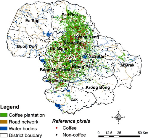
Other datasets include a shapefile map of coffee-growing areas in 2015 (scale: 1/100,00), layers of district boundaries, water bodies, and road networks from the Sub-National Institute of Agricultural Planning and Projection, Vietnam, and annual LULC maps from 1990 to 2020 from the Japan Aerospace Exploration Agency (https://www.eorc.jaxa.jp/ALOS/en/dataset/lulc/lulc_vnm_v2109_e.htm). The coffee map was primarily created from various remotely sensed images, including Landsat and SPOT imageries, and the accuracy of this map has been validated with field survey data. We particularly checked and updated coffee-growing areas that had remained unchanged during the study periods using existing reference sources, including analogous LULC maps, Google Earth high-resolution images across the study region, coffee area statistics, and government reports and publications. A field visit was also carried out in 2020, where locations of coffee patches were collected using a handheld mobile device. This reference map was eventually converted to a raster form and used as the ground reference data for the selection of training samples for image classification and accuracy assessment of the mapping results (Figure 2). The government statistics of coffee growing areas at the district level for 1995, 2005, and 2020 were also collected from Dak Lak’s Department of Agriculture and Rural Development for verification of the association between the satellite-derived coffee area and the official statistics.

Figure 2. Map of coffee-cultivated areas in the study region overlaid with layers of the road network and water bodies. Ground reference pixels (dots) were used for the accuracy assessment of the coffee mapping results.

3. Methods

3.1. Satellite data preprocessing and derivation of predictive variables

The data of Landsat images (surface reflectance level-2 product) stored as digital numbers were firstly multiplied with a scaling factor of 0.0000275 and subtracted by 0.2 to convert it to the surface reflectance (scale from 0 to 1). The geometric corrections were accordingly performed for the 1995 and 2005 Landsat images using the 2020 Landsat image as a reference image using ArcGIS 10.3 package. The correction process was carried out using at least 30 control points uniformly chosen from district features throughout the study region. The results showed that the root mean square error (RMSE) value was smaller than half of the size of a Landsat pixel. The LST data were retrieved from Landsat’s thermal bands 6 (Landsat 5) and 10 (Landsat 8) using the single-channel algorithm (Jiménez‐Muñoz and Sobrino 2003; Sobrino et al. 2004). Because the Landsat data in the region were commonly polluted by clouds, we employed a two-step procedure to create yearly composite images for delineating coffee-cultivated areas in the region. First, the pixels contaminated by dense and cirrus clouds were masked out using the cloud mask product. Second, the temporal pixel-based image composite method using the median value was applied to generate yearly cloud-free composite images to reduce the effects caused by cloud contamination, atmospheric attenuation, and surface directional reflectance (Holben 1986; Huete et al. 2002; Guerschman et al. 2009; Roy et al. 2010; Flood 2013; Mountford et al. 2017).

For each year, a total of 43 variables, including 39 Landsat-based vegetation indices, one Landsat-derived LST, and three topographic indices (i.e. DEM, slope, and aspect), were used in this research for mapping coffee-planted areas (Table 2). The rationale for choosing these parameters was that the DEM, slope, and aspect are topographical parameters that characterize changes in topography and water collection, thus highly related to the land suitability for coffee production. The LST and vegetation indices (e.g. NDVI, EVI, SAVI, and NDWI) have been widely exploited for crop monitoring and yield estimation because they are strongly associated with vegetation health and water stress conditions (Huete 1997; Turner et al. 1999; Gao et al. 2000; Hancock and Dougherty 2007; Kanke et al. 2016; Nolasco et al. 2021). Some of these vegetation and topographic indices have been documented to improve the mapping accuracy in various applications, including crop, forest, and soil classification (Fahsi et al. 2000; Xue and Su 2017; Maleki et al. 2020; Chu et al. 2021; Al-Doski et al. 2022; Kordi and Yousefi 2022; Zeng et al. 2022). All these indices (i.e. 30 m resolution) were stacked into one composite scene (43 bands) and used as independent variables for RF regression analysis to estimate coffee-growing areas.

Table 2. Accuracy assessment results for the coffee classification maps in 2005 and 2017.

Ground reference data (pixels)	Mapping results (pixels)		Total
	Coffee area	Non-coffee area
1995
Coffee	443	57	500
Non-coffee	58	442	500
Total	501	499	1,000
Producer’s accuracy (%)	88.6	88.4
User’s accuracy (%)	88.4	88.6
Overall accuracy (%)	88.5
Kappa coefficient	0.77
2005
Coffee	445	55	500
Non-coffee	54	446	500
Total	499	501	1,000
Producer’s accuracy (%)	89.0	89.2
User’s accuracy (%)	89.2	89.0
Overall accuracy (%)	89.1
Kappa coefficient	0.78
2020
Coffee	435	65	500
Non-coffee	66	434	500
Total	501	499	1,000
Producer’s accuracy (%)	87.0	86.8
User’s accuracy (%)	86.8	87.0
Overall accuracy (%)	86.9
Kappa coefficient	0.74

3.2. Ensemble machine learning algorithm

The RF regression method was selected in this research to investigate coffee-growing areas, based on its primary advantages over other machine-learning algorithms (e.g. linear regression, logistic regression, ANN, SVM, and RNN), including non-parametric nature, high degree of prediction accuracy, capability to determine the variable importance (i.e. the contribution of each feature variable to the model prediction), and ability to handle a large volume of datasets within a relatively short computing time (Ver Hoef et al. 2001; Liaw and Wiener 2002; Prasad et al. 2006; Ishwaran 2007; Roy and Larocque 2012; Belgiu and Dragut 2016; Mi et al. 2017). This algorithm, using the ensemble learning method for regression (Breiman 2001; Tibshirani et al. 2002), combines predictions from multiple machine-learning algorithms to make a more accurate prediction than a single model. It is known as the most commonly used method for solving complex prediction tasks. A set of decision trees is constructed from training samples using the bootstrapping technique to perform the regression, leaving the remaining samples (from the training dataset) for model testing. By intensively learning training samples, the algorithm can discover specific trends and patterns in the dataset. Once the optimal trends and patterns are determined, it is possible to predict accurate future instances (Breiman et al. 1984; Breiman 2001). To reduce the computation time and evaluate a variable’s relevance for prediction, the random-forest predictor importance analysis based on a Gini impurity measure (Loh 2002, Loh and Shih 1999; Louppe et al. 2013) was first applied using the training dataset to extract a minimal set of discriminative predictor variables or determine predictor variables important for the model. The greater importance estimates indicate more important predictors. The relationship between the dependent variable (i.e. coffee-planted areas) and independent variables (i.e. Landsat satellite and DEM-derived indices) can be expressed using the following equation: $$\mathbf{Y}=f(\mathbf{X},\beta )+\epsilon ,$$ where, Y is the dependent variable, determined by independent variables X, β are unknowns, and ε is the error term.

In this research, a total of 20,000 training pixels (i.e. 10,000 samples for each class of coffee-planted areas and non-coffee areas) was randomly chosen from the government’s inventory coffee-growing map, synchronized with those from the composite scene of independent variables. Of these training samples, 70% and 30% of the data were respectively used for model training and testing. Because the accuracy of RF relies on the optimal number of trees, to ensure the number of trees is sufficiently large to stabilize the mean squared error (MSE) rate, 1,000 trees were used in the RF model based on trial and error results. In addition, because the computation time increases linearly with the number of trees and variables, to efficiently reduce the computational cost of data processing, we performed the estimation of predictor importance using the permutation algorithm to determine the influence of each dependent variable in the model for predicting the response (Breiman et al. 1984; Loh 2002b; Ishwaran 2007). Only variables that greatly influence predictions were used for the modeling. The 10-fold cross-validation was also processed to evaluate the model performance by dividing the data into 10 folds of training and testing sets to train and test the model, respectively. The iteration is repeated until each fold of such 10 folds has been used as the testing dataset. The mean squared error (MSE) is used as an indicator for evaluating the model performance.

3.3. Threshold determination and accuracy evaluation

The prediction results of coffee-planted areas (obtained from RF regression) were an image scene, showing the pixel values ranging between 0 and 1, indicating the proportion of coffee-growing area in each pixel. A hardening process was thus applied to convert a mixed pixel to a pure pixel with respect to the desired coffee class or non-coffee class. The threshold was determined based on the intersection between the producer’s and user’s accuracies calculated from the error matrix. To avoid the inclination of selecting the same pixels for model training and mapping accuracy assessment, we excluded training pixels from the selection of pixels used for the accuracy assessment. 1,000 pixels (500 pixels for each class) were randomly extracted from the ground reference map to calculate the producer’s and user’s accuracies with an incremental interval of 0.05 between 0.1 and 0.9. The intersection point between the two curves of the producer’s and user’s accuracies was utilized as a threshold value to classify coffee-planted areas. For assessing the mapping results, we utilized the overall accuracy and Kappa coefficient, which were widely used in the field of remote sensing and map comparison for accuracy assessment (Congalton 1991; Pontius and Millones 2011; Congalton and Green 2019).

4. Results and discussion

4.1. Importance of predictive variables

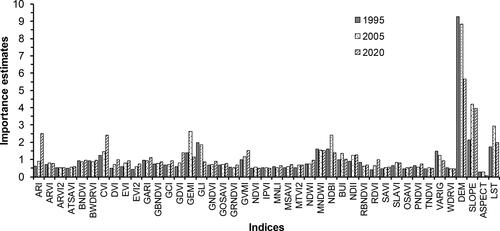
The results of predictor importance analysis for the 1995, 2005, and 2022 datasets showed that 10 out of 43 variables both had variable importance values greater than 0.7 (Figure 3). These variables, including the atmospherically resistant vegetation index (ARVI), green atmospherically resistant vegetation index (GARI), green leaf index (GLI), global vegetation moisture index (GVMI), modified normalized difference water index (MNDWI), normalized difference infrared index (NDII), specific leaf area vegetation index (SLAVI), DEM, SLOPE, and LST, were thus chosen for RF regression analysis. Specifically, the ARVI is developed to correct atmospheric influences in regions with a high content of atmospheric aerosol and air pollution (Tanre et al. 1992). The GARI is more sensitive to the chlorophyll concentration than NDVI and ARVI and is useful to measure the rate of photosynthesis and monitor plant stress (Gitelson et al. 1996). The GLI originally designed to measure wheat cover characterizes soil or non-living features and green leaves or stems (Louhaichi et al. 2001). The GVMI is suggested for the retrieval of vegetation water content (Ceccato et al. 2002). The MNDWI is designed for the detection of water bodies while diminishing built-up areas (Xu 2006). The NDII is sensitive to changes in the water content of plant canopies, which is suitable for crop agricultural management, forest canopy monitoring, and vegetation stress identification (Hardisky et al. 1983). The SLAVI is proposed to estimate specific leaf area (Lymburner et al. 2000) because it is strongly correlated with the volume and height of vegetation, net photosynthesis, net primary production, and leaf area index (Broge and Leblanc 2001; Yu et al. 2010). The DEM characterizes topographic variations, as being the most distinctive factor affecting the land suitability for coffee plantation allocation. Likewise, the slope (derived from DEM) measures the steepness of a feature, and also characterises slope suitability levels for coffee cultivation, which is identified as a yield limiting factor, especially in undrained or eroded elevated areas (FAO 1996). The LST represents the inherent physical processes of energy and water exchange, and has a strong negative association with NDVI as it affects crop phenology and yields (Jackson et al. 1981; Sandholt et al. 2002; Gusso 2018).

Figure 3. Importance estimates of predictive variables.

4.2. Model performance and classification accuracies

The results of 10-fold cross-validation showed that the MSE values achieved for the 1995, 2005, and 2020 datasets were 0.087, 0.093, and 0.0097, respectively. The larger MSE values were observed for 1995, mainly attributed to mixed-pixel problems caused by the expansion of coffee-planted areas and coffee agroforestry systems into forested areas. The spectral confusion between coffee and other industrial crops could consequently increase MSE values between the estimates and the actual observations. The model coefficients for each year were used to estimate the probability of coffee-planted areas for 1995, 2005, and 2020, respectively. The results for each year were an image scene, where the pixel value is a continuous number between 0 to 1, indicating the proportion of coffee area within a pixel. The thresholds of 0.82, 0.78, and 0.81, which were obtained from the intersection of the producer’s and user’s accuracies with a searching range from 0.1 to 0.9, were applied to the 1995, 2005, and 2020 prediction maps to convert mixed pixels to pure pixels concerning two desired classes of coffee or non-coffee.

The accuracies of mapping results were verified in two ways. Firstly, the classification maps were assessed using 1,000 random pixels randomly extracted from the ground reference map to compare with those pixels synchronized from the classification maps. The comparison results showed that the overall accuracy and Kappa coefficient achieved for 1995 were respectively 88.5% and 0.77, while the values for 2005 and 2020 were 89.1% and 0.78, and 86.9% and 0.74, respectively (Table 2). Of 1,000 reference pixels used to check the per-class accuracy of classification maps, the producer’s and user’s accuracies obtained for the 1995 dataset were 88.6% and 88.4%, while the values for the 2005 and 2020 datasets were 89.0% and 89.2%, and 87.0% and 86.8%, respectively. In general, the mapping results were slightly lower for 2020 because this year’s coffee acreage was more spatially dispersed throughout the province due to its expansion into other cropland areas and forests.

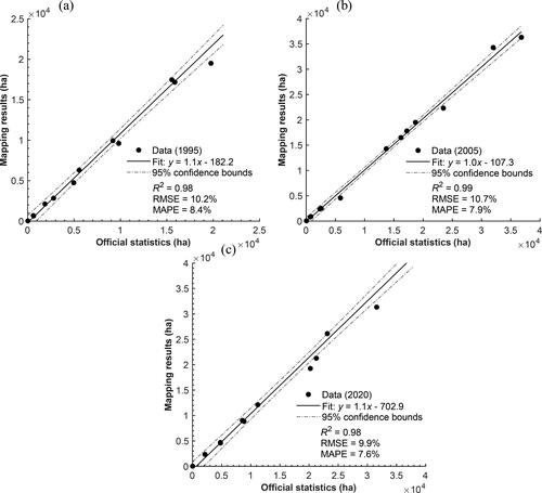
Secondly, to check for consistency, the government’s statistics on coffee-planted areas were compared, district by district, to the satellite-derived coffee areas for 1995, 2005, and 2020. The overall results showed a slight overestimation, in all cases. The relative errors in area, achieved from the area comparisons between these two datasets, were 7.8% for 1995, 1.1% for 2005, and 6.4% for 2020, respectively. Overall, at the district level, the two datasets had a high degree of agreement (Figure 4). The correlation coefficient of determination (R²) values of the fitted models generally explained more than 98% of the variance for 1995, 2005, and 2020 datasets (P-value < 0.001). The RMSPE and MAPE values for 1995 were 10.2% and 8.4%, while values for 2005 and 2020 were respectively 10.7% and 7.9%, and 9.9% and 7.6%, indicating a good consistency between the satellite-derived coffee area and the government’s statistics. The cause of some outliers in scatterplots indicating greater or decreased discrepancies was mainly attributed to mixed-pixel issues, especially in districts, such as M’ Drak, Lak, and Krong Bong, where coffee was less cultivated, and coffee fields were relatively small and highly fragmented.

Figure 4. Relationship between coffee cultivated areas, obtained from the classification of Landsat and DEM-derived indices, and government’s coffee area statistics: (a) 1995, (b) 2005, and (c) 2020.

Overall, this research’s methodology is concentrated on large-scale and crop-specific mapping of coffee plantations as a complicated target using the moderate-resolution Landsat archives to generate multitemporal thematic information on coffee-growing areas over a heterogeneous landscape. In contrast to most earlier satellite-based studies, which focused on typical food crops, such as wheat, corn, and rice, our research burrows into a large-scale classification and decadal change detection of a perennial coffee crop, primarily investigated by a few studies using Landsat and Sentinel images in Central America and Southeast Asian countries (Cordero‐Sancho and Sader 2007; Ortega-Huerta et al. 2012; Kawakubo and Machado 2016; Tridawati et al. 2020; Maskell et al. 2021; Le et al. 2022). With the recent release of higher spatiotemporal resolution Sentinel-1 Synthetic Aperture Radar (SAR) and Sentinel-2 optical data since 2014, we see the integration of these two datasets for more accurate and scalable mapping of coffee-growing areas and monitoring short-term changes in cultivation areas and plant phenology over a large area, especially in cloudy tropical regions, has become feasible (Jia et al. 2014; Escobar-López et al. 2022). However, this is problematic because the unavailability of long-term historical Sentinel-1 and 2 archives places limitations on an analysis of multi-decadal changes in agricultural practices.

To the best of our knowledge, the methods given in this work represent an initial attempt at regional delimitation of coffee-producing areas and decennial changes in agricultural practices through the utilization of a large number of indexes derived from DEM and cloud-free annual Landsat composite datasets with the aid of machine-learning techniques. The merit of image composition is that it chooses the optimal approximation for each pixel in spectral space, thus minimizing the impact of outlier pixels while retaining the spectral relationship between bands. Our research findings also demonstrate the effectiveness of the RF algorithm for classification of coffee plantations from the satellite composite image using only the 10 most important factors (i.e. vegetation, LST, and topographic indices). These results have coincided with previous studies that demonstrate the value of using remotely-sensed vegetation and surface temperature variables in relief-conditioned locations for improved classification of specific crops, including coffee (Langford and Bell 1997; Sesnie et al. 2008; Schmitt-Harsh 2013; Schmitt-Harsh et al. 2013; Chemura et al. 2017a, Cordero‐Sancho and Sader 2007; Hunt et al. 2020; Miranda et al. 2020).

Compared to recent research employing moderate remote sensing data (e.g. Landsat and SPOT) that have mistakenly identified coffee-planted areas as natural forests, orchards, and perennial trees (Cayuela et al. 2006; Stibig et al. 2007; Ortega-Huerta et al. 2012; Kawakubo and Pérez Machado 2016; Kelley et al. 2018; Hunt et al. 2020), our methods yield reasonably good results, but also reveal a challenge for accurately identifying small patches of coffee plantations, mostly due to topographic effects, low spatial resolution of satellite images, and complicated coffee-farming systems in which coffee fields are often intercropped with other perennials (e.g. nut trees, tea, cacao, mulberries, and peppers). This diversification in terms of coffee height strata and crown closure influences the spectral coffee signature in a variety of ways, subsequently misclassifying coffee fields as other woodland trees due to similar crowns. On the other hand, there are coffee parcels that have not been properly updated with ground reference data can also contribute to the increased mapping error as indicated by lower producer’s and user’s accuracies in 2020. Another issue with our approach is that it cannot accurately depict complex coffee-growing landscapes using a composite image since coffee plants’ spectral signatures alter with phenological cycle and age. Although attempts have been made to separate the coffee from other crops and perennials in the study region using the time-series vegetation data (derived from SPOT-VGT), the results reveal consistently unsuccessful isolating of coffee plantations as a result of temporal confusion among cropping patterns (Stibig et al. 2007; Nguyen et al. 2020). Given these difficulties in classification of coffee plantations in the study region, our efforts are still being made to improve the model accuracy by exploiting multiple biophysical variables acquired from multi-date imageries of different sensors.

4.3. Geographic distribution and decadal changes of coffee planted areas

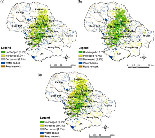
The classification results showed the spatial distributions of areas planted with coffee in 1995, 2005, and 2020 (Figure 5), which are spatially comparable to those on the government’s reference map. In general, coffee has been grown in districts that have an altitude above 300 m with mild weather conditions suitable for growing coffee. Areas cultivated for coffee were relatively dispersed in 1995 (Figure 5a), but much more intensively in 2005 and 2020 (Figures 5b, c). Mapping results for these years were compared to examine decadal changes in areas planted with coffee between these periods (i.e. 1995−2005, 2005−2020, and 1995−2020). The results showed that the coffee area remained broadly unchanged over the period 1995−2020, amounting to approximately 90,749 ha (or 6.9% of the total area of 13,315,199.3 ha), whilst the values for the periods 1995−2005 and 2005−2020 were 6.2% and 10.3%, respectively (Figure 6). Between 1995 and 2020, the total area under coffee grew by approximately 135,520 ha (or 10.3% of the province’s total area). Specifically, newly cultivated coffee areas in the 1995−2005 and 2005−2020 periods were 7% (or 92,508 ha) and 6.7% (or 88,164 ha) respectively, which were mostly observed in districts of the province’s central territories as a result of the conversion of forests to coffee plantations. In contrast, a very small proportion of the coffee acreage (2.1%) declined over these 26 years (1995−2020), and approximately 2.8% and 2.9% for 1995–2005 and 2005–2020, respectively. This decline is primarily attributable to the fact that old coffee trees are grown in steep areas (>15%), where soils are unsuitable and irrigation is inadequate for coffee production, such that the coffee had been cleared for other purposes. These declining areas were dispersed across the study area, particularly in the southern and eastern parts of the study area.

Figure 5. Spatial distributions of coffee cultivated areas in (a) 1995, (b) 2005, and (c) 2020.

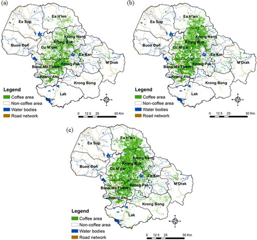
Figure 6. Changed cafe areas between (a) 1995 and 2005, (b) 2005 and 2020, and (c) 1995 and 2020. The percentage refers to the total area of the study region (1,315,199.3 ha).

On the whole, the main driving force of such an expansion of coffee acreage has been attributed to the conversion of forests into coffee plantations due to the suitability of basalt soils for large-scale coffee production and the high profitability of coffee grains for export in the global market (Koninck 1999; D’haeze et al. 2005; Meyfroidt et al. 2013; Dang and Kawasaki 2017; Kissinger 2020). The region’s total coffee production had nearly doubled over the course of 26 years from 107,735 ha in 1995 to 209,955 ha in 2020, in which a higher proportion of the increase in coffee acreage was observed for the period 1995−2005 (1.6%), compared to that of 1.2% for the 2005−2020 period (DLSO 2020). In addition, the expansion of coffee-producing areas may also be caused by the quickening rate of population growth resulting from uncontrolled immigration from other provinces, particularly the central and northern parts of the country, boosted by high coffee prices on the world’s coffee market over the past two decades (DLSO 2020; GSO 2020).

5. Conclusions

The findings of this study confirmed the potential application of our mapping approach to spatially delineate coffee-growing areas, and evaluate decadal changes in coffee-farming practices from 1995 to 2020 using Landsat and DEM-derived indices. The RF-based mapping results, derived from image classification using 10 variables selected based on the analysis of predictor importance, compared with the ground reference data confirmed strong agreement between the two datasets, with the overall accuracy and Kappa coefficient greater than 88.5% and 0.74, respectively. Such findings have also been reaffirmed by the good agreement between the satellite-based coffee area and the government’s coffee area statistics at the district level. From 2000 to 2020, the coffee area increased by approximately 135,520 ha, mostly in the study region’s central districts. This expansion was mainly due to the benefits of the price of coffee on the market and to the demographic growth accelerated by the immigration of persons from other regions. This research eventually led to the recognition of the merit of the use of Landsat-based LST and vegetation indices and topographic variables for coffee mapping using the RF machine-learning algorithm in Vietnam’s Central Highlands. Such a mapping approach could provide quantitative information on spatial distributions of coffee-producing areas and multidecadal changes in farming practices, which was helpful to agronomists and policymakers in addressing crop management and agricultural planning problems in the region.

Disclosure statement

No potential conflict of interest was reported by all authors.

References

- Adriana S. 2019. Top coffee producing countries. Quebec, Canada.
- Al-Doski J, Hassan FM, Mossa HA, Najim AA. 2022. Incorporation of digital elevation model, Normalized Difference Vegetation Index, and Landsat-8 data for land-use/land-cover mapping. Photogramm Eng Remote Sensing. 88(8):507–516.
- Ali A. 2021. Data-driven based machine learning models for predicting the deliverability of underground natural gas storage in salt caverns. Energy. 15229:120648.
- Ashburn P. 1978. The vegetative index number and crop identification. Proceedings of the LACIE Symposium Proceedings of the Technical Session.
- Baret F, Guyot G. 1991. Potentials and limits of vegetation indexes for LAI and APAR assessment. Remote Sens Environ. 35(2-3):161–173.
- Belgiu M, Drăguţ L. 2016. Random forest in remote sensing: a review of applications and future directions. ISPRS J Photogramm Remote Sens. 114:24–31.
- Breiman L. 2001. Random forests. Machine Learning. 45(1):5–32.
- Breiman L, Friedman J, Olshen R, Stone C. 1984. Classification and regression trees. New York: Hall.
- Broge NH, Leblanc E. 2001. Comparing prediction power and stability of broadband and hyperspectral vegetation indices for estimation of green leaf area index and canopy chlorophyll density. Remote Sens Environ. 76(2):156–172.
- Cairns M. 2017. Shifting cultivation policies: balancing environmental and social sustainability.
- Caruana R, Karampatziakis N, Yessenalina A. 2008. An empirical evaluation of supervised learning in high dimensions.
- Caruana R, Niculescu-Mizil A. 2006. An empirical comparison of supervised learning algorithms. Proceedings of the 23rd International Conference on Machine Learning - ICML '06. 06/25; p. 161–168.
- Cayuela L, Benayas JMR, Echeverria C. 2006. Clearance and fragmentation of tropical montane forests in the Highlands of Chiapas, Mexico (1975-2000). For Ecol Manage. 226(1-3):208–218.
- Ceccato P, Flasse S, Gregoire JM. 2002. Designing a spectral index to estimate vegetation water content from remote sensing data - Part 2. Validation and applications. Remote Sens Environ. 82(2-3):198–207.
- CGIAR. 2016. The drought crisis in the Central Highlands of Vietnam. Hanoi, Vietnam.
- Chemura A, Mutanga O, Dube T. 2017a. Integrating age in the detection and mapping of incongruous patches in coffee (Coffea arabica) plantations using multi-temporal Landsat 8 NDVI anomalies. Int J Appl Earth Obs Geoinf. 57:1–13.
- Chemura A, Mutanga O, Dube T. 2017b. Remote sensing leaf water stress in coffee (Coffea arabica) using secondary effects of water absorption and random forests. Phys Chem Earth. 100:317–324.
- Chu L, Jiang CL, Wang TW, Li ZX, Cai CF. 2021. Mapping and forecasting of rice cropping systems in central China using multiple data sources and phenology-based time-series similarity measurement. Adv Space Res. 68(9):3594–3609.
- Claverie M, Vermote EF, Franch B, Masek JG. 2015. Evaluation of the Landsat-5 TM and Landsat-7 ETM + surface reflectance products. Remote Sens Environ. 169:390–403.
- Congalton RG. 1991. A review of assessing the accuracy of classifications of remotely sensed data. Remote Sens Environ. 37(1):35–46.
- Congalton RG, Green K. 2019. Assessing the accuracy of remotely sensed data: Principles and practices, Third Edition (3rd ed.). CRC Press. https://doi.org/10.1201/9780429052729
- Cordero‐Sancho S, Sader SA. 2007. Spectral analysis and classification accuracy of coffee crops using Landsat and a topographic‐environmental model. Int J Remote Sens. 28(7):1577–1593.
- Crippen RE. 1990. Calculating the vegetation index faster. Remote Sens Environ. 34(1):71–73.
- D’haeze D, Deckers J, Raes D, Phong TA, Loi HV. 2005. Environmental and socio-economic impacts of institutional reforms on the agricultural sector of Vietnam. Agricult Ecosyst Environ. 105(1-2):59–76.
- Dang AN, Kawasaki A. 2017. Integrating biophysical and socio-economic factors for land-use and land-cover change projection in agricultural economic regions. Ecol Modell. 344:29–37.
- DLSO 2020. Statistical yearbook of Dak Lak. Dak Lak Department of Statistics, Buon Ma Thuot, Vietnam.
- Dorren LKA, Maier B, Seijmonsbergen AC. 2003. Improved Landsat-based forest mapping in steep mountainous terrain using object-based classification. For Ecol Manage. 183(1-3):31–46.
- Eiumnoh A, Shrestha RP. 2000. Application of DEM data to Landsat image classification: evaluation in a tropical wet-dry landscape of Thailand. Photogramm Eng Remote Sens. 66:297–304.
- Escobar-López A, Castillo-Santiago MÁ, Hernández-Stefanoni JL, Mas JF, López-Martínez JO. 2022. Identifying coffee agroforestry system types using multitemporal Sentinel-2 data and auxiliary information. Remote Sens. 14(16):3847.
- Fahsi A, Tsegaye T, Tadesse W, Coleman T. 2000. Incorporation of digital elevation models with Landsat-TM data to improve land cover classification accuracy. For Ecol Manage. 128(1-2):57–64.
- FAO. 1996. Guidelines for land-use planning. Food and Agriculture Organization of the United Nations, Rome, Italy.
- Feng M, Sexton JO, Huang CQ, Masek JG, Vermote EF, Gao F, Narasimhan R, Channan S, Wolfe RE, Townshend JR. 2013. Global surface reflectance products from Landsat: assessment using coincident MODIS observations. Remote Sens Environ. 134:276–293.
- Flood N. 2013. Seasonal composite Landsat TM/ETM plus images using the medoid (a multi-dimensional median). Remote Sens. 5(12):6481–6500.
- Gao BC. 1996. NDWI - A normalized difference water index for remote sensing of vegetation liquid water from space. Remote Sens Environ. 58(3):257–266.
- Gao X, Huete AR, Ni WG, Miura T. 2000. Optical-biophysical relationships of vegetation spectra without background contamination. Remote Sens Environ. 74(3):609–620.
- Ge GBT, Shi ZJ, Zhu YJ, Yang XH, Hao YG. 2020. Land use/cover classification in an arid desert-oasis mosaic landscape of China using remote sensed imagery: performance assessment of four machine learning algorithms. Global Ecol Conserv. 22:e00971.
- Gitelson AA. 2004. Wide Dynamic Range Vegetation Index for remote quantification of biophysical characteristics of vegetation. J Plant Physiol. 161(2):165–173. Epub 2004/03/17.
- Gitelson AA, Gritz Y, Merzlyak MN. 2003. Relationships between leaf chlorophyll content and spectral reflectance and algorithms for non-destructive chlorophyll assessment in higher plant leaves. J Plant Physiol. 160(3):271–282. Epub 2003/05/17.
- Gitelson AA, Kaufman YJ, Merzlyak MN. 1996. Use of a green channel in remote sensing of global vegetation from EOS-MODIS. Remote Sens Environ. 58(3):289–298. Epub 1996/12/01.
- Gitelson A, Merzlyak M, Zur Y, Stark R, Gritz U. 2001. Non-destructive and remote sensing techniques for estimation of vegetation status. Third European Conference on Precision Agriculture, Montpelier, France.
- Glenn EP, Nagler PL, Huete AR. 2010. Vegetation index methods for estimating evapotranspiration by remote sensing. Surv Geophys. 31(6):531–555.
- Gobron N, Pinty B, Verstraete MM, Widlowski JL. 2000. Advanced vegetation indices optimized for up-coming sensors: design, performance, and applications. IEEE Trans Geosci Remote Sensing. 38(6):2489–2505.
- GSO. 2020. Statistical yearbook of Vietnam.
- Guerschman JP, Hill MJ, Renzullo LJ, Barrett DJ, Marks AS, Botha EJ. 2009. Estimating fractional cover of photosynthetic vegetation, non-photosynthetic vegetation and bare soil in the Australian tropical savanna region upscaling the EO-1 Hyperion and MODIS sensors. Remote Sens Environ. 113(5):928–945.
- Gusso A. 2018. Canopy temperatures distribution over soybean crop fields using satellite data in the Amazon biome frontier. Eur J Remote Sens. 51(1):901–910. Epub 2018/01/01.
- Haboudane D, Miller JR, Pattey E, Zarco-Tejada PJ, Strachan IB. 2004. Hyperspectral vegetation indices and novel algorithms for predicting green LAI of crop canopies: modeling and validation in the context of precision agriculture. Remote Sens Environ. 90(3):337–352.
- Hancock DW, Dougherty CT. 2007. Relationships between blue- and red-based vegetation indices and leaf area and yield of alfalfa. Crop Sci. 47(6):2547–2556.
- Hardisky M, Klemas V, Smart a 1983. The influence of soil salinity, growth form, and leaf moisture on the spectral radiance of Spartina alterniflora canopies. Photogramm Eng Remote Sens. 48:77–84.
- Holben BN. 1986. Characteristics of maximum-value composite images from temporal AVHRR data. Int J Remote Sens. 7(11):1417–1434. Epub 1986/11/01.
- Huete A. 1997. A comparison of vegetation indices over a global set of TM images for EOS-MODIS. Remote Sens Environ. 59(3):440–451.
- Huete AR. 1988. A soil-adjusted vegetation index (SAVI). Remote Sens Environ. 25(3):295–309. Epub 1988/08/01.
- Huete A, Didan K, Miura T, Rodriguez EP, Gao X, Ferreira LG. 2002. Overview of the radiometric and biophysical performance of the MODIS vegetation indices. Remote Sens Environ. 83(1-2):195–213.
- Hunt ER, Daughtry CST, Eitel JUH, Long DS. 2011. Remote sensing leaf chlorophyll content using a visible band index. Agron J. 103(4):1090–1099.
- Hunt DA, Tabor K, Hewson JH, Wood MA, Reymondin L, Koenig K, Schmitt-Harsh M, Follett F. 2020. Review of remote sensing methods to map coffee production systems. Remote Sens. 12(12):2041.
- ICO. 2020. World coffee production. International Coffee Organization, London, UK.
- Ishwaran H. 2007. Variable importance in binary regression trees and forests. Electron J Statist. 1:519–537.
- Jackson RD, Idso SB, Reginato RJ, Pinter PJ. 1981. Canopy temperature as a crop water stress indicator. Water Resour Res. 17(4):1133–1138.
- Jain P, Coogan S, Subramanian S, Crowley M, Taylor SW, Flannigan M. 2020. A review of machine learning applications in wildfire science and management. Environ. Rev. 28(4): 478–505
- Jia K, Liang SL, Zhang N, Wei XQ, Gu XF, Zhao X, Yao YJ, Xie XH. 2014. Land cover classification of finer resolution remote sensing data integrating temporal features from time series coarser resolution data. ISPRS J Photogramm Remote Sens. 93:49–55.
- Jiang ZY, Huete AR, Didan K, Miura T. 2008. Development of a two-band enhanced vegetation index without a blue band. Remote Sens Environ. 112(10):3833–3845.
- Jiménez‐Muñoz JC, Sobrino JA. 2003. A generalized single‐channel method for retrieving land surface temperature from remote sensing data. J Geophys Res. 108(D22): 4688–4694.
- Kanke Y, Tubana B, Dalen M, Harrell D. 2016. Evaluation of red and red-edge reflectance-based vegetation indices for rice biomass and grain yield prediction models in paddy fields. Precision Agric. 17(5):507–530.
- Kaufman YJ, Tanre D. 1992. Atmospherically resistant vegetation index (Arvi) for EOS-MODIS. IEEE Trans Geosci Remote Sensing. 30(2):261–270.
- Kawakubo FS, Machado RPP. 2016. Mapping coffee crops in southeastern Brazil using spectral mixture analysis and data mining classification. Int J Remote Sens. 37(14):3414–3436.
- Kelley LC, Pitcher L, Bacon C. 2018. Using google earth engine to map complex shade-grown coffee landscapes in northern Nicaragua. Remote Sens. 10(6):952.
- Kim D-C, Hoang TQ. 2013. Development of coffee production and land mobility in Dak Lak, Vietnam. J Econ Geograph Soc Korea. 16:359–371.
- Kissinger G. 2020. Policy responses to direct and underlying drivers of deforestation: examining rubber and coffee in the Central Highlands of Vietnam. Forests. 11(7):733.
- Koninck R. 1999. Deforestation in Viet Nam/Rodolphe de Koninck. International Development Research Centre. Ottawa, Ontario, Canada.
- Kordi F, Yousefi H. 2022. Crop classification based on phenology information by using time series of optical and synthetic-aperture radar images. Remote Sens Appl: soc Environ. 27:100812. Epub 2022/08/01.
- Körting TS, Garcia Fonseca LM, Câmara G. 2013. GeoDMA-geographic data mining analyst. Comput Geosci. 57:133–145.
- Krishnan S. 2017. Sustainable coffee production. Oxford Res. Ency. of Environ.l Sci., Oxford University Press. https://doi.org/10.1093/acrefore/9780199389414.013.224
- Langford M, Bell W. 1997. Land cover mapping in a tropical hillsides environment: a case study in the Cauca region of Colombia. Int J Remote Sens. 18(6):1289–1306.
- Lawson CE, Martí JM, Radivojevic T, Jonnalagadda SVR, Gentz R, Hillson NJ, Peisert S, Kim J, Simmons BA, Petzold CJ, et al. 2021. Machine learning for metabolic engineering: a review. Metab Eng. 63:34–60.
- Le QT, Dang KB, Giang TL, Tong THA, Nguyen VG, Nguyen TDL, Yasir M. 2022. Deep learning model development for detecting coffee tree changes based on sentinel-2 imagery in Vietnam. IEEE Access. 10:109097–109107.
- Liaw A, Wiener M. 2002. Classification and regression by random forest. Rnews.2,18-22. http://CRAN.R-project.org/doc/Rnews.
- Loh W-Y. 2002. Regression trees with unbiased variable selection and interaction detection. Statistica Sin. 12:361–386.
- Loh W-Y, Shih Y-s 1997. Split selection methods for classification trees. Statistica Sin 7:815-840.
- Louhaichi M, Borman MM, Johnson DE. 2001. Spatially located platform and aerial photography for documentation of grazing impacts on wheat. Geocarto Int. 16(1):65–70. Epub 2001/03/01.
- Louppe G, Wehenkel L, Sutera A, Geurts P. 2013. Understanding variable importances in Forests of randomized trees. NIPS'13: Proceedings of the 26th International Conference on Neural Information Processing Systems. 1:431–439.
- Lu Z. 2021. Computational discovery of energy materials in the era of big data and machine learning: a critical review. Materials Reports: energy. 1(3):100047. Epub 2021/06/28.
- Lymburner L, Beggs PJ, Jacobson CR. 2000. Estimation of canopy-average surface-specific leaf area using Landsat TM data. Photogramm Eng Remote Sens. 66:183–191.
- Maleki S, Khormali F, Mohammadi J, Bogaert P, Bodaghabadi MB. 2020. Effect of the accuracy of topographic data on improving digital soil mapping predictions with limited soil data: an application to the Iranian loess plateau. Catena. 195:104810.
- Mansaray LR, Wang F, Huang J, Yang L, Kanu AS. 2020. Accuracies of support vector machine and random forest in rice mapping with Sentinel-1A, Landsat-8 and Sentinel-2A datasets. Geocarto Int. 35(10):1088–1108.
- Martinez‐Castillo C, Astray G, Mejuto JC, Simal‐Gandara J. 2020. Random forest, artificial neural network, and support vector machine models for honey classification. eFood. 1(1):69–76.
- Maskell G, Chemura A, Nguyen H, Gornott C, Mondal P. 2021. Integration of Sentinel optical and radar data for mapping smallholder coffee production systems in Vietnam. Remote Sens. Environ. 266:112709.
- Mboga N, Persello C, Bergado JR, Stein A. 2017. Detection of informal settlements from VHR satellite images using convolutional neural networks. Proceedings of the 2017 IEEE International Geoscience and Remote Sensing Symposium (IGARSS); 23–28 July 2017.
- Meyfroidt P, Phuong VT, Anh HV. 2013. Trajectories of deforestation, coffee expansion and displacement of shifting cultivation in the Central Highlands of Vietnam. Global Environ Change-Human Policy Dimensions. 23(5):1187–1198.
- Meyfroidt P, Vu TP, Hoang VA. 2013. Trajectories of deforestation, coffee expansion and displacement of shifting cultivation in the Central Highlands of Vietnam. Global Environ Change. 23(5):1187–1198.
- Mi C, Huettmann F, Guo Y, Han X, Wen L. 2017. Why choose Random Forest to predict rare species distribution with few samples in large undersampled areas? Three Asian crane species models provide supporting evidence. PeerJ. 5:e2849. Epub 2017/01/18.
- Miller ED, Jones ML, Henry MM, Stanfill B, Jankowski E. 2019. Machine learning predictions of electronic couplings for charge transport calculations of P3HT. AIChE J. 65(12):e16760.
- Miranda JR, Alves MD, Pozza EA, Neto HS. 2020. Detection of coffee berry necrosis by digital image processing of landsat 8 oli satellite imagery. Int J Appl Earth Obs Geoinf. 85:101983.
- Mohajane M, Costache R, Karimi F, Pham QB, Essahlaoui A, Nguyen H, Laneve G, Oudija F. 2021. Application of remote sensing and machine learning algorithms for forest fire mapping in a Mediterranean area. Ecol Indic. 129:107869.
- Mountford GL, Atkinson PM, Dash J, Lankester T, Hubbard S. 2017. Chapter 4 - Sensitivity of vegetation phenological parameters. From Satellite Sensors to Spatial Resolution and Temporal Compositing Period. In: Sensitivity analysis in earth observation modelling, edited by George P. P. and Prashant K. S., Elsevier, Amsterdam, Netherlands; p. 75–90.
- Müller D. 2002. Land use dynamics in the central highlands of Vietnam: a spatial model combining village survey data with satellite imagery interpretation. Agricult Econ. 27(3):333–354.
- Nguyen HT, Nguyen LV, de Bie CAJM, Ciampitti IA, Nguyen DA, Nguyen MV, Nieto L, Schwalbert R, Nguyen LV. 2020. Mapping maize cropping patterns in Dak Lak, Vietnam through MODIS EVI time series. Agronomy. 10:478. https://doi.org/10.3390/agronomy10040478
- Nolasco M, Ovando G, Sayago S, Magario I, Bocco M. 2021. Estimating soybean yield using time series of anomalies in vegetation indices from MODIS. Int J Remote Sens. 42(2):405–421.
- Ortega-Huerta MA, Komar O, Price KP, Ventura HJ. 2012. Mapping coffee plantations with Landsat imagery: an example from El Salvador. Int J Remote Sens. 33(1):220–242. Epub 2012/01/10.
- Peng W, Li S, He Z, Ning S, Liu Y, Su Z. 2019. Random forest classification of rice planting area using multi-temporal polarimetric Radarsat-2 data. Proceedings of the. IGARSS 2019 - 2019 IEEE International Geoscience and Remote Sensing Symposium; 28 July-2 Aug. 2019.
- Pinty B, Verstraete MM. 1992. GEMI: a non-linear index to monitor global vegetation from satellites. Vegetatio. 101(1):15–20.
- Pontius RG, Millones M. 2011. Death to Kappa: birth of quantity disagreement and allocation disagreement for accuracy assessment. Int J Remote Sens. 32(15):4407–4429.
- Prasad AM, Iverson LR, Liaw A. 2006. Newer classification and regression tree techniques: bagging and random forests for ecological prediction. Ecosystems. 9(2):181–199.
- Qi SH, Brown DG, Tian Q, Jiang LG, Zhao TT, Bergen KA. 2009. Inundation extent and flood frequency mapping using LANDSAT imagery and digital elevation models. Gisci Remote Sens. 46(1):101–127.
- Qi J, Chehbouni A, Huete AR, Kerr YH, Sorooshian S. 1994. A modified soil adjusted vegetation index. Remote Sens Environ. 48(2):119–126.
- Richardsons AJ, Wiegand A. 1977. Distinguishing vegetation from soil background information. Photogramm Eng Remote Sens. 43:1541–1552.
- Rodriguez-Galiano VF, Chica-Olmo M, Abarca-Hernandez F, Atkinson PM, Jeganathan C. 2012. Random Forest classification of Mediterranean land cover using multi-seasonal imagery and multi-seasonal texture. Remote Sens Environ. 121:93–107.
- Rondeaux G, Steven M, Baret F. 1996. Optimization of soil-adjusted vegetation indices. Remote Sens Environ. 55(2):95–107.
- Roy DP, Ju JC, Kline K, Scaramuzza PL, Kovalskyy V, Hansen M, Loveland TR, Vermote E, Zhang CS. 2010. Web-enabled Landsat Data (WELD): Landsat ETM plus composited mosaics of the conterminous United States. Remote Sens Environ. 114(1):35–49.
- Roy MH, Larocque D. 2012. Robustness of random forests for regression. J Nonparametric Stat. 24(4):993–1006.
- Roy DP, Wulder MA, Loveland TR, Woodcock CE, Allen RG, Anderson MC, Helder D, Irons JR, Johnson DM, Kennedy R, et al. 2014. Landsat-8: science and product vision for terrestrial global change research. Remote Sens Environ. 145:154–172.
- Saini RK, Ghosh S. 2018. Crop classification on single date Sentinel-2 imagery using random forest and suppor vector machine. Int. Arch. Photogramm. Remote Sens. Spatial Inf. Sci., XLII-5:683–688. https://doi.org/10.5194/isprs-archives-XLII-5-683-2018
- Sandholt I, Rasmussen K, Andersen J. 2002. A simple interpretation of the surface temperature/vegetation index space for assessment of surface moisture status. Remote Sens Environ. 79(2-3):213–224.
- Santos É, Macedo L, Tundisi LL, Ataide JA, Camargo GA, Alves RC, Oliveira MBPP, Mazzola PG. 2021. Coffee by-products in topical formulations: a review. Trends Food Sci Technol. 111:280–291.
- Schmitt-Harsh M. 2013. Landscape change in Guatemala: driving forces of forest and coffee agroforest expansion and contraction from 1990 to 2010. Appl Geogr. 40:40–50.
- Schmitt-Harsh M, Sweeney SP, Evans TP. 2013. Classification of coffee-forest landscapes using landsat TM imagery and spectral mixture analysis. Photogramm Eng Remote Sens. 79(5):457–468.
- Sesnie SE, Gessler PE, Finegan B, Thessler S. 2008. Integrating Landsat TM and SRTM-DEM derived variables with decision trees for habitat classification and change detection in complex neotropical environments. Remote Sens Environ. 112(5):2145–2159.
- Sheykhmousa M, Mahdianpari M, Ghanbari H, Mohammadimanesh F, Ghamisi P, Homayouni S. 2020. Support vector machine versus random forest for remote sensing image classification: a meta-analysis and systematic review. IEEE J Sel Top Appl Earth Observ Remote Sens. 13:6308–6325.
- Shiferaw H, Bewket W, Eckert S. 2019. Performances of machine learning algorithms for mapping fractional cover of an invasive plant species in a dryland ecosystem. Ecol Evol. 9(5):2562–2574. Epub 2019/03/21.
- Sobrino JA, Jimenez-Munoz JC, Paolini L. 2004. Land surface temperature retrieval from LANDSAT TM 5. Remote Sens Environ. 90(4):434–440. 30
- Son N-T, Chen C-F, Chen C-R, Minh V-Q. 2017. Assessment of Sentinel-1A data for rice crop classification using random forests and support vector machines. Geocarto Int. 33(6):587–601 https://doi.org/10.1080/10106049.2017.1289555.
- Speiser JL. 2021. A random forest method with feature selection for developing medical prediction models with clustered and longitudinal data. J Biomed Inform. 117:103763. Epub 2021/03/31.
- Statista. 2019. Global leading countries based on coffee area. Food and Agriculture Organization of the United Nations, New York, United States.
- Stibig H-J, Belward AS, Roy PS, Rosalina-Wasrin U, Agrawal S, Joshi PK, Beuchle R, Fritz S, Mubareka S, Giri C, et al. 2007. A land-cover map for South and Southeast Asia derived from SPOT-VEGETATION data. J Biogeography. 34(4):625–637.
- Tan JB, Zuo JQ, Xie XY, Ding MQ, Xu ZK, Zhou FB. 2021. MLAs land cover mapping performance across varying geomorphology with Landsat OLI-8 and minimum human intervention. Ecol Inf. 61:101227.
- Tanre D, Holben BN, Kaufman YJ. 1992. Atmospheric correction algorithm for Noaa-Avhrr products – Theory and application. IEEE Trans Geosci Remote Sensing. 30(2):231–248.
- Thao NT, Khoi DN, Denis A, Viet LV, Wellens J, Tychon B. 2022. Early prediction of coffee yield in the central highlands of Vietnam using a statistical approach and satellite remote sensing vegetation biophysical variables. Remote Sens. 14(13):2975.
- Tibshirani R, Hastie T, Narasimhan B, Chu G. 2002. Diagnosis of multiple cancer types by shrunken centroids of gene expression. Proc Natl Acad Sci U S A. 99(10):6567–6572. Epub 2002/05/16.
- Tridawati A, Wikantika K, Susantoro TM, Harto AB, Darmawan S, Yayusman LF, Ghazali MF. 2020. Mapping the distribution of coffee plantations from multi-resolution, multi-temporal, and multi-sensor data using a random forest algorithm. Remote Sens. 12(33):3933. https://doi.org/10.3390/rs12233933
- Tucker CJ. 1979. Red and photographic infrared linear combinations for monitoring vegetation. Remote Sens Environ. 8(2):127–150.
- Tucker CJ, Elgin JH, McMurtrey JE, Fan CJ. 1979. Monitoring corn and soybean crop development with hand-held radiometer spectral data. Remote Sens Environ. 8(3):237–248. Epub 1979/08/01.
- Turner DP, Cohen WB, Kennedy RE, Fassnacht KS, Briggs JM. 1999. Relationships between leaf area index and Landsat TM spectral vegetation indices across three temperate zone sites. Remote Sens Environ. 70(1):52–68.
- Uttaruk Y, Laosuwan T. 2016. Remote sensing based vegetation indices for estimating above ground carbon sequestration in orchards. AgricultForest. 62(4):93–201.
- Velásquez D, Sánchez A, Sarmiento S, Toro M, Maiza M, Sierra B. 2020. A method for detecting coffee leaf rust through wireless sensor networks, remote sensing, and deep learning: case study of the Caturra Variety in Colombia. Appl Sci. 10(2):697.
- Velásquez D, Sánchez A, Sarmiento S, Velásquez C, Toro M, Montoya E, Trefftz H, Maiza M, Sierra B. 2021. A cyber-physical data collection system integrating remote sensing and wireless sensor networks for coffee leaf rust diagnosis. Sensors. 21(16):5474. https://doi.org/10.3390/s21165474
- Ver Hoef JM, Cressie N, Fisher RN, Case TJ. 2001. Uncertainty and spatial linear models for ecological data. In C. T. Hunsaker, M. F. Goodchild, M. A. Friedl & T. J. Case (Eds.), Spatial uncertainty in ecology: implications for remote sensing and GIS applications. New York, NY: Springer New York; p. 214–237.
- Wang F-m, Huang J-f, Tang Y-l, Wang X-z 2007. New vegetation index and its application in estimating leaf area index of rice. Rice Sci. 14(3):195–203. Epub 2007/09/01.
- Wright MN, Ziegler A. 2017. ranger: a fast implementation of random forests for high dimensional data in C++ and R. J Stat Soft. 77(1):1–17. https://doi.org/10.18637/jss.v077.i01
- Xu HQ. 2006. Modification of normalised difference water index (NDWI) to enhance open water features in remotely sensed imagery. Int J Remote Sens. 27(14):3025–3033.
- Xue JR, Su BF. 2017. Significant remote sensing vegetation indices: a review of developments and applications. J Sens. 2017:1–17. Epub 2017/05/23.
- Yang CG, Everitt JH, Bradford JM. 2007. Airborne hyperspectral imagery and linear spectral unmixing for mapping variation in crop yield. Precision Agric. 8(6):279–296.
- Yang Z, Willis P, Mueller R. 2008. Impact of band-ratio enhanced AWIFS image on crop classification accuracy.
- Yin H, Tan B, Frantz D, Radeloff VCC. 2022. Integrated topographic corrections improve forest mapping using Landsat imagery. Int J Appl Earth Obs Geoinf. 108:102716.
- Yu YF, Saatchi S, Heath LS, LaPoint E, Myneni R, Knyazikhin Y. 2010. Regional distribution of forest height and biomass from multisensor data fusion. J Geophys Res Biogeosci. 115:0–12.
- Zeng YL, Hao DL, Huete A, Dechant B, Berry J, Chen JM, Joiner J, Frankenberg C, Bond-Lamberty B, Ryu Y, et al. 2022. Optical vegetation indices for monitoring terrestrial ecosystems globally. Nat Rev Earth Environ. 3(7):477–493.
- Zha Y, Gao J, Ni S. 2003. Use of normalized difference built-up index in automatically mapping urban areas from TM imagery. Int J Remote Sens. 24(3):583–594.