Observation of the vertical structure of atmospheric boundary layer in subtropical UHI by radiosonde

Abstract

Existing studies on the urban heat island (UHI) effect tend to focus on the planar scale. However, the UHI effect has obvious three-dimensional properties. This research focuses on the vertical structure of UHI. The study combined big data from sounding balloon and surface measurements in the Database for Atmospheric and Hydrologic Research, Taiwan. Data organization and classification were conducted using the Python programming language, the NumPy mathematical function library, and the Pandas data manipulation library. Results confirmed the existence of the atmospheric boundary layer and the canopy. Furthermore, the temperature inversion of the atmospheric boundary layer fell between heights of 130 m and 667 m. The height of the inversion is affected by the wind speed and cloudiness. Thereby demonstrating that the inversion fluctuates with weather scenario changes. The research results can be applied as the direction of urban planning thinking for urban heat island countermeasures.

Keywords:

• urban heat island
• height of the inversion
• vertical structure of UHI
• big data
• urban climate factors
• atmospheric boundary layer
• urban canopy

1. Introduction

The urban heat island (UHI) effect is a unique phenomenon in temperature distribution in which the temperatures in urban areas are higher than those in the surrounding suburbs (Landsberg 1982; T. R. Oke 1982). Anthropogenic heat, reduction in vegetation cover, high building density, evaporation reduction, the widespread use of asphalt pavement, and the high heat capacity and endothermic properties of building materials all exacerbate the UHI effect (Battista and Mauri 2016; Guan et al. 2011; Qin 2015; Santamouris 2014; Stewart 2011). Buildings and road paving are the primary driving forces of the high temperatures (Zhao et al. 2017) as well as the annual increases in maximum temperatures (Hulley 2012). Relevant studies have pointed out that changes in surface pavement features are a primary cause of the UHI effect and that surface temperatures could be lowered by using pavement materials that absorb less heat (Benrazavi et al. 2016).

In previous studies, the influencing factors of urban heat island temperature are wind field, humidity, and radiation temperature etc. In this study, since the research site is located in the subtropical zone, humidity is an important factor affecting urban thermal comfort (Armson et al. 2012; de Abreu-Harbich et al. 2015; Niu et al. 2015; Z. Tan et al. 2016). Changes in urban ground surface features influence the local climate by altering the surface energy balance and boundary layers. Urban structure, development intensity, and building material types also impact the intensity of the UHI effect (Stone and Rodgers 2001). Different types of land use, such as urban centers, parks, and various suburban areas, result in significant changes in net radiation, thermal storage, and sensible and latent heat, which lead to local climate changes (Fehrenbach et al. 2001). Although planting vegetation can reduce UHI effects and convert the heat in the surrounding environment into latent heat, thereby lowering nearby temperatures, the increased enthalpy reduces human comfort. A number of studies have examined the positive and negative influences of vegetation and green spaces on urban thermal environments.

From the perspective of urban meteorology, the UHI effect has obvious three-dimensional properties, so research into the dissipation of heat islands should not focus exclusively on planar scales. The influence of environmental geomorphological features on urban boundary layers is still unknown. Hsin-Hua Hsin-Hua Tsai (2018) employed an unmanned aerial vehicle to collect the climate factors of vertical structures with different surface features in urban areas and observed the results of local-scale UHI vertical structures, which reflected that the heat flows of two representative environmental features differed and a close relationship exists between the parameter distributions and surface features of urban vertical structure sections. Many research has also shown that urban environment features affect not only temperatures near the ground surface but also the boundary layers (Zhu et al. 2016). Relevant studies also discuss the influence of aerosol transport by seasons or daytime through the structure of the atmospheric boundary layer (Miao et al. 2018; Miao et al. 2015) . Some have explored the urban-rural differences in boundary layer and ozone concentration (Zong et al. 2022).

T. R. Oke (1976) proposed two scales for the measurement of UHIs: the boundary layer and the canopy. The urban boundary layer is influenced by land use or urban surfaces. It is above the canopy and referred to the local or meso-scale. The altitude of the urban boundary layer is generally defined based on the thermal inversion (Bianco and Wilczak 2002).

Inversions can be roughly divided into advection, subsidence, or radiation inversions. When warm air flows horizontally above colder air, it creates an advection inversion. In cold cloudless conditions, the rapid cooling of the ground and the resulting dropping surface temperatures hinder vertical movement in the atmosphere, which leads to radiation inversions (Schnelle et al. 2015).

The atmospheric boundary layer is influenced by the micro-scale below it and the meso-scale above it. The urban canopy is located roughly between the ground and the tops of the buildings, which is referred to as the micro-scale and is strongly influenced by urban geometric shapes and micro-scale airflows and energy exchanges (Arnfield 2003; T. R. Oke 1976), as well as the ground surface and morphological and human parameters (Arnfield 2003; Renard et al. 2019). Heat island temperatures are generally measured in the canopy and boundary-layer (Yin et al. 2018).

The urban heat island is defined as a city center that is warmer than surrounding suburbs (Landsberg 1982; T. R. Oke 1982). Studying the spatiotemporal variation of UHI and its causes is of great significance for comprehension of urban climate, planning and green development, and disaster reduction (Yang et al. 2022). However, the temperature change in the vertical sky is unknown, this study aimed to investigate the correlation between vertical structures of UHI and weather patterns. This study would explore the correlation between temperature inversion and weather factors, to interpret the issues affecting the UHI and canopy height. This study aimed to investigate the correlation between the height of the inversion vertical thermal structures and weather patterns. We obtained large quantities of data from an atmospheric and hydrologic research database and used statistical methods to investigate the changes in UHI boundary layer and canopy fluctuations and characteristics under various conditions. This study would explore the correlation between temperature inversion and weather factors, to interpret the issues affecting the UHI and canopy height.

An effective approach is required to utilize urban big data to solve urban problems (Liu et al. 2020), such as urban planning, traffic, environmental protection, energy consumption, social applications, and urban public safety and protection (Zheng et al. 2014). Seidel et al. (2010) advocated that the current climatology of atmospheric boundary layer height could be based on automated algorithms applying big data. This study discusses the variation of the boundary layer and the canopy UHI under different meteorological variables through radiosonde big data. Differences of UHI in urban canopy and boundary layers under different seasons and weather scenarios are studied.

2. Methods

This research employed radiosonding data from the Database for Atmospheric and Hydrologic Research, Taiwan and big data from a radiosonde carried by a sounding balloon to analyze the atmospheric boundary layer and canopy of UHIs. We applied this data to investigate the correlation between UHI vertical structure and weather factors. The main concept and methodology of this paper is to process the big data of urban climate factors with statistical methods.

2.1. Research area

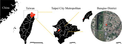
The Taipei Metropolitan is located in northern Taiwan. (25°1′48″N, 121°37′48″E) is the metropolis of the capital, Taipei City. It includes Taipei City, New Taipei City, and Keelung City and has a total area of 2,457.11 km². According to the civil affairs departments of the three cities, a total of 6,803,949 people resided in the Taipei Metropolitan Area in June, 2022, which represents roughly 30% of the country’s population. The Taipei Metropolitan Area has a subtropical climate, which is hot and humid. Southwest monsoon prevails in summer. Average temperatures in the summer reach 29-30 °C with 70-80% humidity (Central Weather Bureau, Ministry of Transportation and Communications, 2021). The Taipei Metropolitan locates in the basin. It is not easy to dissipate the heat, so its heat and humidity will easily keep in the city. Hot summers, multiple typhoons, and torrential rain characterize this local climate.

The weather station where we released a sounding balloon carrying a radiosonde is located in Banqiao District of New Taipei City (25°00′40″N, 121°26′45″E) (Figure 1), near the Dahan River and the Fuzhou artificial wetlands. Taipei Metropolis is highly urbanized, and the buildings near the weather station are all old apartment buildings that are four to seven stories high, which makes this station the perfect location to explore fluctuations in the atmospheric boundary layer and canopy.

Figure 1. Location of Banqiao weather station.

2.2. Construction of digital database for urban vertical structures

2.2.1. Sounding and surface data

The Database for Atmospheric and Hydrologic Research, Taiwan, is compiled by the Central Weather Bureau, which has an automatic upper-air sounding system at the Banqiao weather station that performs upper-aid observation operations every day at 8:00 and 20:00(UTC + 8 in Taipei), thereby collecting two items of data per day. Banqiao Observatory is located at longitude 121°26’1.57”E, latitude 24°59’57.5”N, and its observation items are temperature, dew point, humidity, air pressure, air pressure trends and characteristics, air pressure variables, extreme temperatures, rainfall, wind direction and speed, cloud shape, cloud cover, cloud base height, visibility, ground conditions, special phenomena. Hourly weather data obtained at 8:00 and 20:00 served as the data for the surface data. We compiled sounding and surface data obtained during 2009 to 2019. The sounding data parameters included air pressure, temperature, humidity, wind speed, wind direction, and height of parameter measurements. The surface data also included rainfall and cloud cover. The height of the sounding data in this study is below 1000 m. Compared with the 70 km diameter range of Taipei Metropolis, the air exploration balloons are obviously collecting data still above the metropolitan area, that should show the phenomenon of urban heat island.

2.2.2. Climate scenario categorization

Weather patterns have a profound impact on site airflow movement. To regulate microclimates, the characteristics of different types of weather must be understood, and they must be categorized into different control scenarios. Clear days and cloudy days imply differences in radiation balance, which cause varying day and night temperature differences and wind speed differences. These two scenarios reflect how the areas process the heat load of the urban environment during the day, the cooling of structures, and nighttime comfort.

According to the Central Weather Bureau’s categorization of cloud cover (10 deciles), cloud cover amounts of 8, 9, and 10 are seen as high cloud cover, and cloud cover amounts of 0, 1, and 2 are seen as low cloud cover. Based on the overall data distributions, this studies defined humidity above 85% as high and humidity below 65% as low, while wind speed above 4 m/s was considered high and wind speed below 1.5 m/s was considered low.

2.2.3. Data manipulation and graphing

Data organization and classification was conducted using the Python programming language, the NumPy mathematical function library, and the Pandas data manipulation library. We filtered out data with missing fields and abnormal values. Based on the total cloud cover in the surface data, we eliminated data missing the cloud cover parameter and overlaid 11 years of sounding data and surface data.

Graphs and tables of substantial amounts of data were made and output using Matplotlib, which is a visualization operation interface of Python and its numerical mathematics expansion pack NumPy. Through mathematical calculations, big data processing, and graphing capabilities, we output relevant graphs and tables based on our study objective.

2.3. Acquisition of inversion data

The atmospheric boundary layer (ABL) is traditionally defined as the ‘part of the troposphere that is directly influenced by the presence of the Earth’s surface, and responds to surface forcing with a time scale of about an hour or less’ (Stull 1988). It is closely related to atmospheric fields such as pollutant diffusion and weather forecasting (Moreira et al. 2020).

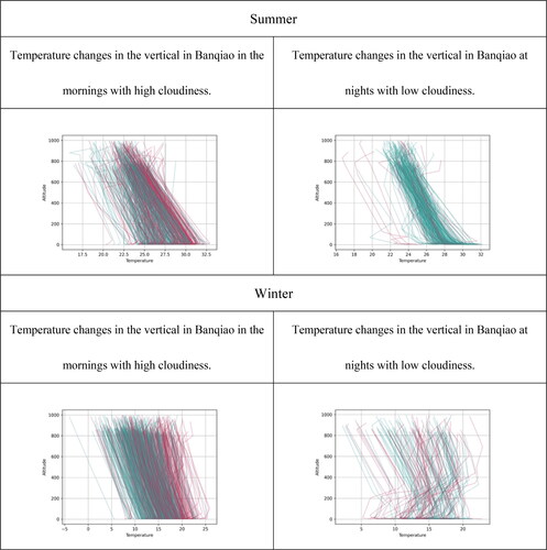
For atmospheric boundary layer analysis, there are many traditional and non-traditional ways to obtain the PBL height. Such as ‘parcel method’, the level of the maximum vertical gradient of potential temperature, the base of an elevated temperature (T) inversion. Different methods often produce different climate ABL height estimates (Seidel et al. 2010). According to literature, the altitude of the boundary layer is defined based on the thermal inversion (Bianco and Wilczak 2002). An inversion is a region where the temperature increases with altitude (Kassomenos et al. 2014). In the troposphere, the temperature generally declines with the altitude, whereas in a thermal inversion, the temperature of the atmosphere increases with the altitude. The inversions mentioned in this study refer to atmospheric temperatures increasing with the altitude, meaning an inversion in temperature. Not all probes have elevated reversals, but if present, the bottom will act as an upper bound for the mix below, so it can be considered the ABL height (Seidel et al. 2010). The inversion point was obtained using the Python math module. The slopes of all points and adjacent points on the line segment were calculated, and the inversion point occurred where the slope turned from negative to positive. The first inversion point indicated the height of the canopy, whereas the second inversion point indicated the height of the boundary layer. This studies organized and graphed the data by Python. Using red curves to represent inversions, we observed the changes in the vertical temperature data. Figures 2 show the temperature distributions in Banqiao on summer and winter mornings with high cloud cover and on summer and winter nights with low cloud cover. These served as preparatory work for the subsequent discussion on the arithmetic means and standard deviations of boundary layer thickness.

Figure 2. The Temperature Inversion with high or low Cloudiness in Summer/Winter.

2.4. Means and standard deviations of the height of the inversion

To explore the fluctuations in the height of the inversion presented by big data and the mean the height of the inversion or the thickness of UHI under different weather factors, we employed statistical methods to calculate the means and standard deviations of the height of the inversion resulting from different weather factors. The arithmetic mean is the quotient obtained from dividing the sum of a set of data by the number of data items, as shown in Equation (1)(1) $$\mathrm{\mu }=\frac{x_1+x_2+\dots +x_N\mathrm{ }}{N}=\frac{{\sum }_{i=1}^N{x}_i}{N}$$(1) : (1) $$\mathrm{\mu }=\frac{x_1+x_2+\dots +x_N\mathrm{ }}{N}=\frac{{\sum }_{i=1}^N{x}_i}{N}$$(1)

The arithmetic mean is a measure of central tendency that represents all observed data using a single value. It is easily affected by extreme values, so we used the standard deviation to examine the degree of dispersion in the boundary layer height data. The formula for the standard deviation is as shown in Equation (2)(2) $${\sigma }_x=\mathrm{ }\sqrt{\frac{1}{n}\mathrm{ }\sum _{i=1}^n{(x_i-{\mu }_x)}^2}$$(2) : (2) $${\sigma }_x=\mathrm{ }\sqrt{\frac{1}{n}\mathrm{ }\sum _{i=1}^n{(x_i-{\mu }_x)}^2}$$(2)

σ_x= standard deviation

μ_x= arithmetic mean

3. Results and analysis

3.1. Investigation of heat island boundary layer and the temperature inversion in Taipei Metropolitan area

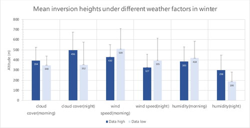
In order to effectively explore the inversion height of the atmospheric boundary layer and canopy under different meteorological variables in the city, we employed Python to perform inversion calculations, the results of which were output to Excel for boundary layer inversion height visualization and analysis. These facilitated observation of UHI boundary layer fluctuations and the influence of different weather factors. Figures 3 and 4 show the bar charts and standard deviations of the mean boundary layer inversion heights resulting from different weather factors in summer and winter. Weather changes will affect the height of the inversion, because the radiosonde data is limited, only two, and the data at 8:00 am represents the end of the entire night-time effect, and the data at 8:00 pm is the end of the entire daytime effect. Therefore, the statistical method could only discuss the influence of the meteorological factors of cloudiness, wind speed and humidity on the atmospheric boundary layer condition.

Figure 3. Mean inversion heights under different weather factors in summer.

Figure 4. Mean inversion heights under different weather factors in winter.

3.1.1. Cloudiness and humidity

The mean inversion heights at night were higher than those in the morning. This was because in the morning, the heat in the city from the day before had dissipated and the surface had yet to receive much radiation. The heights presented at night indicated the total amount of heat accumulated during the day, and the warm air had slowly risen due to convection. Thus, the mean inversion heights at night were higher than those in the morning. On the ground surface it accumulated a particularly high amount of heat, which raised the UHI dome height. Thus, the mean inversion height in the morning was approximately 300 m.

High cloudiness affects radiative heat dissipation, so higher inversion were observed whenever the cloud cover was high, regardless of season. The inversion at night were higher than those in the morning due to slow radiative cooling on nights with high cloud cover; the heat then built up in the urban greenhouse under the clouds, causing heat accumulation and hence higher inversion. We observed significant differences between the inversion heights in the morning and those at night in the winter; this is likely because it was difficult for the long-wave radiation from the surface to penetrate the clouds and dissipate into space. Much of the energy was absorbed and radiated back to earth, which increased surface temperature. Thus, nights with high cloud cover had a ‘warming effect’ that increased the inversion height to 496 m. However, the atmospheric boundary layer seems to be more irregular in terms of the influence of humidity of the inversion height. The humidity is not closely related to the thickness of the entire atmospheric boundary layer.

3.1.2. Wind speed

Wind speed exerted a significant impact on mean inversion height. The mean inversion heights in conditions with high wind speeds were lower than those in conditions with low wind speeds. This was because high wind speeds at the surface blew the heat away. With low wind speeds, the surface temperatures rose, thereby increasing inversion height. Even on winter mornings with low wind speeds, the mean inversion height was 509 m. On summer nights, high wind speeds could effectively reduce inversion height to a mean value of 234 m. In the mornings, the surface had just begun to heat up from solar radiation; the rising temperatures caused the air to increase in volume and decrease in density. The density difference generated buoyancy, which caused the unstable heat source to transfer heat upwards.

Thus, the inversion heights in the morning were higher than those at night regardless of season. The mean inversion heights on winter mornings and nights showed that the extent to which high wind speeds reduced inversion height was not as great as that in summer. As the temperatures in the winter were far lower than those in the summer, the impact of wind speed was not as significant. Nevertheless, low wind speeds could still effectively reduce inversion height.

On the whole, wind speed can effectively reduce inversion height; high wind speeds disperse surface heat directly and quickly restore the temperatures to a declining gradient form, thereby creating a lower inversion. At night, in particular, wind speeds are high and the sun is no longer sending heat into the city. The heat accumulated during the day is dissipated by high wind speeds, so the minimum canopy thickness at high wind speeds was 130 m. In the summer with low wind speeds, the mean inversion height was approximately 382 m, whereas with high wind speeds, the mean inversion height was roughly 201 m. In winter with low wind speeds, the mean inversion height was about 452 m, whereas with high wind speeds, the mean inversion height was approximately 379 m. The difference between the inversion heights at high and low wind speeds was about 251 m.

3.1.3. Mean height and temperature of the inversion phenomenon

From the data above, it is shown that the wind speed has the most significant influence on the height of inversion. Then the temperature value of the inversion will be discussed separately, under high wind speed and low wind speed conditions. Figures 5 and 6 present the mean temperatures in the inversion on summer and winter mornings and nights with high and low wind speeds.

Figure 5. Mean temperature at height of temperature inversion in summer.

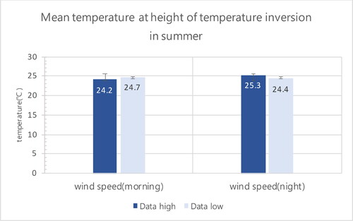
Figure 6. Mean temperature at height of temperature inversion in winter.

The mean temperatures at height of temperature inversion on summer mornings and nights fell between 24 °C and 26 °C. A comparison of the data from mornings with high and low wind speeds with the data in Figure 2 showed that during these times, the mean inversion height and temperature resulting from high wind speeds were 272 m and 24.2 °C, respectively, whereas the mean inversion height and temperature resulting from low wind speeds were 400 m and 24.7 °C. The temperature resulting from low wind speeds was higher by 0.5 °C, and the inversion height was thicker. This is because the low wind speeds did not disperse the heat, causing the structure of the UHI boundary layer to be more solid and contain more heat. In contrast, the structures of the UHI boundary layer at high wind speeds were less solid, but the difference was not significant. At low wind speeds, the difference between morning and night temperatures was only 0.3 °C. The differences in both temperature and inversion height were not significant, showing that significant differences only appeared in summer when the wind speed was high.

Regarding the boundary layer thickness and temperature on mornings and nights in summer with high wind speeds, the mean temperature on nights with high wind speeds was 25.3 °C. The mean boundary layer height dropped from 272 m to 130 m, but the temperature increased by 1.1 °C. This shows that the structures of UHI boundary layers were more solid at night, thereby demonstrating a characteristic phenomenon of UHIs in the summer.

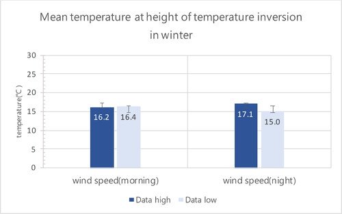
The mean inversion temperatures on winter mornings and nights with high and low wind speeds fell between 15 °C and 17 °C. The mean temperatures on mornings with high and low wind speeds were 16.2 °C and 16.4 °C, respectively, whereas the mean temperatures on nights with high and low wind speeds were 17.1 °C and 15 °C. With high wind speeds, the boundary layer inversion dropped from 430 m in the morning to 327 m at night, whereas with low wind speeds, it dropped from 509 m in the morning to 395 m at night. The temperature only declined slightly. Compared to that in the summer, the thickness of UHI boundary layers resulting from inversions in the winter was significantly greater.

UHI boundary layers resulting from inversions in the winter were thicker. With endless heat generated in urban areas, the temperatures higher up were indeed lower in the winter, that leads to higher temperature and more thickness of the inversion. Thus, both the solidity and height of the inversion were influenced by the season and wind speed. With high wind speeds, the heat was easily blown away, so the vertical inversion structure was less solid and the inversion was thinner.

3.2. Investigation of UHI canopy

3.2.1. Canopy fluctuations

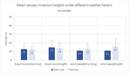
We output the UHI canopy values to Excel for inversion height visualization and analysis. Figures 7 and 8 show bar charts and standard deviations of the mean canopy inversion heights resulting from different weather factors in summer and winter. As can be seen, the influence of different weather factors on canopy fluctuations was not significant; they only caused fluctuations ranging from 10 m to 20 m. Furthermore, the impact of the wind speed variable was similar to that on the UHI—higher wind speeds resulted in lower canopies.

Figure 7. Mean canopy inversion heights under different weather factors in summer.

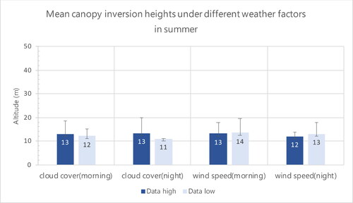
Figure 8. Mean canopy inversion heights under different weather factors in winter.

3.2.2. Mean wind speeds at different heights

We further discuss the mean wind speeds at different heights in the canopy. Figures 9 and 10 show the mean wind speeds and data regarding mean wind speeds at different heights in the summer and winter. We divided the height intervals into 1.5 m (human height), 11-50 m (within the UHI canopy), 50-250 m (between the UHI canopy and boundary layer), 250-450 m (in the UHI boundary layer), and 450-1000 m (above the UHI boundary layer).

Figure 9. Mean wind speeds at different heights in the summer.

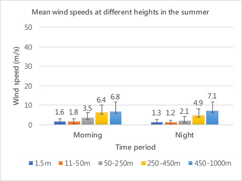
Figure 10. Mean wind speeds at different heights in the winter.

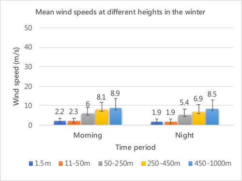
On summer mornings and nights, the mean wind speeds were 1.5 m/s and 1.5 m/s at 1.5 m and 11-50 m, 2.8 m/s at 50-250 m (between the UHI canopy and UHI boundary layer), 5.7 m/s at 250-450 m (in the UHI boundary layer), and 7 m/s at 450-1000 m. On winter mornings and nights, the mean wind speeds were 2 m/s at 1.5 m, 2.1 m/s at 11-50 m, 5.7 m/s at 50-250 m, 7.5 m/s at 250-450 m (in the UHI boundary layer), and 8.7 m/s at 450-1000 m. The mean wind speeds were higher than those in the summer. We found that the wind speed values between the surface and 50 m in the canopy were all relatively low. Based on the data from the radiosonde, we determined that canopy inversion height was influenced by building height, wind speeds at low heights, and human activity.

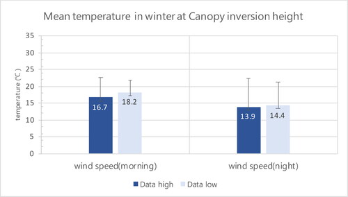
Figures 11 and 12 present the mean temperature in summer and winter at Canopy inversion height. Regardless of wind speed, the mean temperatures on summer mornings and nights were approximately 27 °C, which is about the same as that at 12-14 m in the canopy inversion. Thus, the urban canopy in the summer is subject to UHIs near the surface with more solid structures. The differences between the temperatures on winter mornings and nights were somewhat greater: the temperatures were 16.7-18.2 °C in the morning and dropped to 13.9-14.4 °C at night. The canopy height was 11-15 m, fluctuating somewhat more in the winter, and the temperature was lower. Thus, the urban canopy in the winter is subject to UHIs near the surface with looser structures.

Figure 11. Mean temperature in summer at Canopy inversion height.

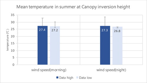
Figure 12. Mean temperature in winter at Canopy inversion height.

3.3. The fluctuation of temperature inversion heights urban in boundary layer and urban canopy

In the sounding balloon data, the heights of the urban boundary layer and urban canopy clearly fluctuate. Using statistical methods, we can identify the factors that influence the boundary layer.

3.3.1. Atmospheric boundary layer

Statistical induction and visualized graphs indicated that cloud cover does not seem to have a significant impact on vertical structures. However, for the most part, the inversion in atmospheric boundary layers are higher in the winter because temperatures higher up are lower, making it easier for urban heat to form clear inversions. Oke (1987) mentioned that the factors influencing UHI boundary layers included increases in short-wave radiation, changes in potential energy, and urbanization characteristics; furthermore, human heat sources and increases in roof heat flux in the urban canopy also indirectly influence boundary layer height.

The inversion heights in atmospheric boundary layer showed that with low wind speeds, the mean inversion height could reach 400 m in the summer, whereas with high wind speeds, the mean boundary layer height could drop to 130 m at the lowest. In summer, the mean inversion height could reach 509 m with low wind speeds, whereas with high wind speeds, the mean inversion height could decline to 327 m. Higher mean wind speeds reduced inversion height regardless of season. High wind speeds could effectively lower the inversion height by about 234 m in the summer night and by 79 m in the winter morning. This indicates that wind speed is a weather factor that can effectively reduce the height of UHI.

Different inversion heights and UHI thicknesses have different meanings. The structural properties of UHI boundary layers are vary depending on the season. UHI boundary layers are thicker in the winter than in the summer, and in day and night comparisons, inversion heights are thinner when the wind speeds are high, and the vertical structures of UHIs are more solid and apparent at night. Urban areas have absorbed a large amount of heat before nighttime, so they continue to release heat at night. When the wind speeds are low, the heat cannot disperse beyond the inversion, so the structure of the UHI boundary layer is more solid. Air movements caused by topographic features are determined by form, such as height, length, width, and the intervals between continuous ridges (Flores Rojas et al. 2018). Thus, urban inversion temperatures will vary depending on the surface features. Observing the inversion heights in atmospheric boundary layer resulting from different weather factors and understanding vertical thermal structures in the atmosphere are therefore crucial for urban planning to disperse heat and humidity.

3.3.2. Canopy

In contrast, the fluctuations in canopy height were not significant, ranging from 10 m to 20 m. The fluctuations in the winter were relatively smaller. If each story is 3 m high, then the buildings surrounding the weather station (which are 4- to 7-story-tall apartment buildings) are about 12-21 m tall, which fits the fluctuating canopy inversion height. Thus, the mean urban canopy inversion height is associated with mean building height. In terms of the mean wind speeds at different heights (Figures 9 and 10), wind speeds at 1.5-50 m near the surface were lower. For buildings emerge some barrier for the wind, thereby disturbing the canopy wind field and resulting in lower wind speeds. Wind speeds declined swiftly, particularly in the winter.

After we divided the data by wind speed, lower canopy inversion heights were found when wind speeds were higher and higher canopy inversion heights were found when wind speeds were lower. Oke (1987) mentioned that canopy inversion heights are lower with higher wind speeds and that as the canopy is influenced by buildings, wind speed is one of the primary factors influencing canopy height. This fits the statistical results of this study. Interpretation of sounding data and their statistics indicate that canopy inversion height is influenced by building height and low wind speeds. The urban canopy includes interactions between buildings; aside from the radiative, thermal, and humidity properties of building materials and the differences caused by urban street canyons, there are likely other differences as well.

3.4. Discussion

Urban-rural temperature differences are influenced by two types of factors: weather factors (such as cloud thickness, humidity, and wind speed) and urban structure factors (such as urban scale, building density, building height, and intervals between buildings). All of these factors have major impacts on the UHI effect (Givoni 1998). Relevant research indicates that changes in urban structure exert a significant influence on urban surface temperature (Kuang et al. 2015). The relatively dense building clusters in commercial districts also absorb the solar radiative heat reflected off one another to a greater extent than that in other areas, causing heat buildup. Thus, urban areas have greater heat absorption areas and more opportunities to absorb and store heat. The thermal properties of urbanization are associated with spatial heterogeneity, and significant differences exist between thermal surface and air temperatures (Shiflett et al. 2017). Increased wind speeds can reduce the UHI effect, improving outdoor comfort and dispersing the pollutants in the air (Emmanuel 2005). Clearly, wind can greatly mitigate the UHI effect (Hsieh et al. 2010; Krüger et al. 2011; Morakinyo et al. 2013). Only adequate winds can effectively blow heat away from its source and prevent local heat accumulation (Hsieh and Huang 2016). The findings of related studies are consistent with that in this study in that high wind speeds can effectively disperse heat accumulated in urban areas, thereby lowering height of the boundary layer.

Essentially, urban climate and road axes are directly associated with building height and their attributes (Krüger et al. 2011), and building height affects urban density, which in turn influences the urban thermal climate (Kakon et al. 2010). In building-dense areas in the subtropics in the summer, in particular, the UHI effect increases discomfort (Zheng Tan et al. 2017). The local wind fields produced by heat are determined by terrain and urban form, and the temperature differences within metropolitan areas are strongly influenced by various microclimates and terrains (Ketterer and Matzarakis 2014). However, it is difficult to discern whether it is the influence of terrain or land use (Landsberg 1982). Thus, changes in altitude and land use all present different microclimate changes. They have also pointed out that terrain exerts a profound impact on the UHI phenomenon (Ketterer and Matzarakis 2014). The significance of urban form is that it expresses the spatial dimensions of urban elements and helps with understanding the influence of urban geometric shapes on radiative heat exchange, air flow, and temperature (T. R. Oke et al. 2017). Furthermore, research on urban thermal environments indicates that the thermal conditions of metropolitan areas are influenced by urban development factors, building density area, land use area, and geographic factors (Chen et al. 2019). The vertical exchanges of heat and humidity in urban and rural areas occur not only on a single plane but also within the thickness of the urban canopy (T. Oke and Canada 2006).

Boundary layer height is an important measure quantifying boundary layer parameters and is crucial in turbulence energy parameterization and weather model forecasting (T. R. Oke 1987). Relevant research has shown that atmospheric structures change with urban form and land use/land cover (LULC) (Liang and Keener 2015). Research has shown that boundary layer inversion height varies with urban land use, urban activity, season, and time of day. That is, the boundary layer fluctuates. However, the canopy remains relatively stable. The boundary layer inversion readings collected by the radiosonde varied significantly; they were sometime very thick or could drop extremely low. In the summer, in particular, humans generate a substantial amount of waste heat in metropolitan areas, so important factors include human influence and the pattern of the metropolitan areas themselves, in addition to weather factors such as season and sunlight. Statistics show that UHI boundary layer heights can range from 130 m to 667 m due to different weather factors, thereby demonstrating that the inversion in atmospheric boundary layer fluctuates. The UHI value in Taipei can be as high as 8 degree C (Chang et al. 2021). Banqiao has a dense population, high anthropogenic waste heat, and high building density. Its urban pattern is common in Taipei, and its conditions are similar to those in other areas within a 25-km radius of Taipei. Based on the boundary layer thickness and vertical structures at single points in Banqiao, we boldly infer that the UHI boundary layer in the Taipei Metropolitan Area is a blanket of uneven thickness rather than the semicircular dome shown in most UHI diagrams.

Using statistical and inductive methods, we derived the mean inversion heights in atmospheric boundary layer and mean temperatures to interpret problems that influence inversion in atmospheric boundary layer and canopy height. Using big data, we categorized inversion phenomena, thereby indicating the existence of the boundary layer and the canopy. Inversion height in atmospheric boundary layer is influenced by cloud cover, and the impact of wind speed is the most regular; High wind speed leads to height reduction of inversions, and the structural solidity of inversion height and UHI thickness vary depending on the season and wind speed. The inversion phenomenon is clear within the boundary layer and the canopy.

Relevant research indicates that the planning and design of urban forms are more important than land cover. Urban planning should therefore focus on mitigating the UHI effect (Yin et al. 2018). The temperature changes in urban areas are influenced by conditions such as the density and height of surrounding buildings, surface material, sunlight conditions, and regional wind (Givoni 1998). Indeed, even small-scale urban areas may form local heat islands, which are closely associated with vertical structures.

4. Conclusions

We interpreted inversion data extracted using Python from big data collected by a radiosonde. The results indicated that building materials, building height, urban activities and climatic scenario influence the fluctuations and properties of the inversion of UHI and canopy. Canopy inversion height is influenced by building height and low wind speeds. The canopy is located around the mean building height and is associated with human activities and low wind speeds.

The solidity of UHI structures varies depending on the season. Specifically, they are thicker in the winter. The thickness of the inversion fluctuates with weather scenario changes. When wind speeds are high, the inversion is thinner, and the vertical structure is more solid and apparent at night. When wind speeds are low, the heat cannot escape from the atmospheric boundary layer, so the structure of the UHI is more solid. High wind speeds can effectively reduce height of inversions. When the wind speed is high, the urban rising thermal energy (UHI) can be quickly taken away, thus weakening the temperature inversion phenomenon and reducing the inversion height. On the contrary, when the wind speed is low, the urban heat cannot be evacuated, resulting in the accumulation of heat energy and increasing the inversion height. High cloud cover affects the dispersion of radiative heat, causing surface heat to accumulate and resulting in a higher inversion. The roof heat flux of the urban canopy increases, which also indirectly influences inversion height. The changes in high altitude temperatures are deeply influenced by surface land use and weather factors. Using big data from a radiosonde carried by a sounding balloon, we analyzed the inversion in the atmospheric boundary layer and canopy heights resulting from different variables to under-stand the vertical heat flow system and propose effective methods for UHI reduction and urban planning. This study is limited to the analysis of the vertical structure of the urban heat island based on the data from a single station. In the future, it is hoped to expand to multi-point data adoption analysis, to expand the completeness and persuasiveness of the 3D description of the heat island. In addition, it is also to further explore the difference in the impact of urban land use on thermal characteristics at the vertical structural scale of the heat island.

Acknowledgements

The authors would like to thank for the support of the Ministry of Science and Technology of Taiwan [MOST—110-2221-E-027-018-MY2] and ‘Research Center of Energy Conservation for New Generation of Residential, Commercial, and Industrial Sectors’ of the Higher Education Sprout Project by the Ministry of Education (MOE) in Taiwan.

Disclosure statement

No potential conflict of interest was reported by the authors.

Additional information

Funding

The authors would like to thank for the support of the Ministry of Science and Technology of Taiwan [MOST—110-2221-E-027-018-MY2] and ‘Research Center of Energy Conservation for New Generation of Residential, Commercial, and Industrial Sectors’ of the Higher Education Sprout Project by the Ministry of Education (MOE) in Taiwan.

References

- Armson D, Stringer P, Ennos AR. 2012. The effect of tree shade and grass on surface and globe temperatures in an urban area. Urban For Urban Green. 11(3):245–255.
- Arnfield AJ. 2003. Two decades of urban climate research: a review of turbulence, exchanges of energy and water, and the urban heat island. Int J Climatol. 23(1):1–26.
- Battista G, Mauri L. 2016. Numerical study of buoyant flows in street canyon caused by ground and building heating. Energy Procedia. 101(Supplement C):1018–1025.
- Benrazavi RS, Binti Dola K, Ujang N, Sadat Benrazavi N. 2016. Effect of pavement materials on surface temperatures in tropical environment. Sustain Cities Soc. 22(Supplement C):94–103.
- Bianco L, Wilczak JM. 2002. Convective boundary layer depth: improved measurement by Doppler radar wind profiler using fuzzy logic methods. J Atmos Oceanic Technol. 19(11):1745–1758. https://doi.org/10.1175/1520-0426(2002)019<1745:CBLDIM>2.0.CO;2.
- Central Weather Bureau, Ministry of Transportation and Communications. 2021. https://www.cwb.gov.tw/V8/C/.
- Chang ME, Zhao ZQ, Chang HT. 2021. Relationship among fractional vegetation cover, land use and urban heat island using Landsat 8 in Taipei, Taiwan. GeoJournal Library. 129:81–95.
- Chen Y-C, Liao Y-J, Yao C-K, Honjo T, Wang C-K, Lin T-P. 2019. The application of a high-density street-level air temperature observation network (HiSAN): the relationship between air temperature, urban development, and geographic features. Sci Total Environ. 685:710–722.
- de Abreu-Harbich LV, Labaki LC, Matzarakis A. 2015. Effect of tree planting design and tree species on human thermal comfort in the tropics. Landscape Urban Plann. 138:99–109.
- Emmanuel R. 2005. An urban approach to climate sensitive design: strategies for the Tropics
- Fehrenbach U, Scherer D, Parlow E. 2001. Automated classification of planning objectives for the consideration of climate and air quality in urban and regional planning for the example of the region of Basel/Switzerland. Atmos Environ. 35(32):5605–5615.
- Flores Rojas JL, Pereira Filho AJ, Karam HA, Vemado F, Masson V. 2018. Effects of explicit urban-canopy representation on local circulations above a tropical mega-city. Boundary-Layer Meteorol. 166(1):83–111.
- Givoni B. 1998. Climate considerations in building and urban design. Van Nostrand Reinhold: John Wiley.
- Guan B, Ma B, Qin F. 2011. Application of asphalt pavement with phase change materials to mitigate urban heat island effect. Paper presented at the ISWREP 2011 Proceedings of 2011 International Symposium on Water Resource and Environmental Protection.
- Hsieh C-M, Chen H, Ooka R, Yoon J, Kato S, Miisho K. 2010. Simulation analysis of site design and layout planning to mitigate thermal environment of riverside residential development. Build Simul. 3(1):51–61.
- Hsieh C-M, Huang H-C. 2016. Mitigating urban heat islands: a method to identify potential wind corridor for cooling and ventilation. Comput Environ Urban Syst. 57:130–143.
- Hsin-Hua Tsai C-HH. 2018. Surveying the Thermal Properties of an Urban Heat Island Vertical Structure Influenced by Subtropical Solar Radiation. Paper presented at the International Conference on Environment and Natural Science (ICENS), Taipei, Taiwan.
- Hulley ME. 2012. 5 - The urban heat island effect: causes and potential solutions. In: Zeman F, editor. Metropolitan sustainability. Woodhead Publishing; p. 79–98. Sawston(Cambridge) : Woodhead Publishing.
- Kakon AN, Nobuo M, Kojima S, Yoko T. 2010. Assessment of thermal comfort in respect to building height in a high-density city in the tropics. Am J Eng Appl Sci. 3(3):545–551.
- Kassomenos PA, Paschalidou AK, Lykoudis S, Koletsis I. 2014. Temperature inversion characteristics in relation to synoptic circulation above Athens, Greece. Environ Monit Assess. 186(6):3495–3502.
- Ketterer C, Matzarakis A. 2014. Human-biometeorological assessment of the urban heat island in a city with complex topography – the case of Stuttgart, Germany. Urban Clim. 10:573–584.
- Krüger EL, Minella FO, Rasia F. 2011. Impact of urban geometry on outdoor thermal comfort and air quality from field measurements in Curitiba, Brazil. Build Environ. 46(3):621–634.
- Kuang W, Liu Y, Dou Y, Chi W, Chen G, Gao C, Yang T, Liu J, Zhang R. 2015. What are hot and what are not in an urban landscape: quantifying and explaining the land surface temperature pattern in Beijing, China. Landscape Ecol. 30(2):357–373.
- Landsberg HE. 1982. The urban climate. Available from: https://www.scopus.com/inward/record.uri?eid=2-s2.0-0020404164&partnerID=40&md5=f5587bb4f7010435271e156ee1262691.
- Liang MS, Keener TC. 2015. Atmospheric feedback of urban boundary layer with implications for climate adaptation. Environ Sci Technol. 49(17):10598–10606.
- Liu J, Li T, Xie P, Du S, Teng F, Yang X. 2020. Urban big data fusion based on deep learning: an overview. Inf Fusion. 53:123–133.
- Miao Y, Guo J, Liu S, Zhao C, Li X, Zhang G, Wei W, Ma Y. 2018. Impacts of synoptic condition and planetary boundary layer structure on the trans-boundary aerosol transport from Beijing-Tianjin-Hebei region to northeast China. Atmos Environ. 181:1–11.
- Miao Y, Hu X-M, Liu S, Qian T, Xue M, Zheng Y, Wang S. 2015. Seasonal variation of local atmospheric circulations and boundary layer structure in the Beijing-Tianjin-Hebei region and implications for air quality. J Adv Model Earth Syst. 7(4):1602–1626.
- Morakinyo TE, Balogun AA, Adegun OB. 2013. Comparing the effect of trees on thermal conditions of two typical urban buildings. Urban Clim. 3:76–93.
- Moreira GdA, Guerrero-Rascado JL, Bravo-Aranda JA, Foyo-Moreno I, Cazorla A, Alados I, Lyamani H, Landulfo E, Alados-Arboledas L. 2020. Study of the planetary boundary layer height in an urban environment using a combination of microwave radiometer and ceilometer. Atmos Res. 240:104932.
- Niu J, Liu J, Lee T-c, Lin Z (, Mak C, Tse K-T, Tang B-s, Kwok KC. 2015. A new method to assess spatial variations of outdoor thermal comfort: onsite monitoring results and implications for precinct planning. Build Environ. 91:263–270.
- Oke TCanada. 2006. Initial guidance to obtain representative meteorological observations at urban sites.
- Oke TR. 1976. The distinction between canopy and boundary‐layer urban heat islands. Atmosphere. 14(4):268–277.
- Oke TR. 1982. The energetic basis of the urban heat island (Symons Memorial Lecture, 20 May 1980). Q J R Meteorol Soc. 108(455):1–24. https://www.scopus.com/inward/record.uri?eid=2-s2.0-0020371056&partnerID=40&md5=693696300a399c5179461d96ba5026d7.
- Oke TR. 1987. Boundary layer climates. London(UK): Routledge.
- Oke TR, Mills G, Christen A, Voogt JA. 2017. Urban climates. Cambridge: Cambridge University Press.
- Qin Y. 2015. A review on the development of cool pavements to mitigate urban heat island effect. Renewable Sustainable Energy Rev. 52(Supplement C):445–459.
- Renard F, Alonso L, Fitts Y, Hadjiosif A, Comby J. 2019. Evaluation of the effect of urban redevelopment on surface urban heat islands. Remote Sen. 11(3):299.
- Santamouris M. 2014. Cooling the cities – a review of reflective and green roof mitigation technologies to fight heat island and improve comfort in urban environments. Sol Energy. 103(Supplement C):682–703.
- Schnelle KB, Dunn RF, Ternes ME. 2015. Air pollution control technology handbook. CRC Press.
- Seidel DJ, Ao CO, Li K. 2010. Estimating climatological planetary boundary layer heights from radiosonde observations: Comparison of methods and uncertainty analysis. J Geophys Res. 115:D16.
- Shiflett SA, Liang LL, Crum SM, Feyisa GL, Wang J, Jenerette GD. 2017. Variation in the urban vegetation, surface temperature, air temperature nexus. Sci Total Environ. 579:495–505.
- Stewart ID. 2011. Redefining the urban heat island. Available from https://open.library.ubc.ca/collections/24/items/1.0072360.
- Stone B, Rodgers MO. 2001. Urban form and thermal efficiency: how the design of cities influences the urban heat island effect. J Am Plann Assoc. 67(2):186–198.
- Stull RB. 1988. An introduction to boundary layer meteorology. Available from https://www.scopus.com/inward/record.uri?eid=2-s2.0-85040878654&partnerID=40&md5=b5974e07faffdf42edd29b364244db18.
- Tan Z, Lau KK-L, Ng E. 2017. Planning strategies for roadside tree planting and outdoor comfort enhancement in subtropical high-density urban areas. Build Environ. 120(Supplement C):93–109.
- Tan Z, Lau KKL, Ng E. 2016. Urban tree design approaches for mitigating daytime urban heat island effects in a high-density urban environment. Energy Build. 114:265–274.
- Yang Y, Guo M, Ren G, Liu S, Zong L, Zhang Y, Zheng Z, Miao Y, Zhang Y. 2022. Modulation of wintertime canopy urban heat island (CUHI) intensity in Beijing by synoptic weather pattern in planetary boundary layer. JGR Atmos. 127(8):e2021JD035988.
- Yin C, Yuan M, Lu Y, Huang Y, Liu Y. 2018. Effects of urban form on the urban heat island effect based on spatial regression model. Sci Total Environ. 634:696–704.
- Zhao Z-Q, He B-J, Li L-G, Wang H-B, Darko A. 2017. Profile and concentric zonal analysis of relationships between land use/land cover and land surface temperature: case study of Shenyang, China. Energy Build. 155(Supplement C):282–295.
- Zheng Y, Capra L, Wolfson O, Yang H. 2014. Urban computing: concepts, methodologies, and applications. ACM Trans Intell Syst Technol. 5(3):1–55.
- Zhu X, Ni G, Cong Z, Sun T, Li D. 2016. Impacts of surface heterogeneity on dry planetary boundary layers in an urban-rural setting. J Geophys Res Atmos. 121(20):12,164–12,179.
- Zong L, Yang Y, Xia H, Gao M, Sun Z, Zheng Z, Li X, Ning G, Li Y, Lolli S. 2022. Joint occurrence of heatwaves and ozone pollution and increased health risks in Beijing, China: role of synoptic weather pattern and urbanization. Atmos Chem Phys. 22(10):6523–6538.