Impacts of climatic variability on surface water area observed by remotely sensed imageries in the Red River Basin

Abstract

Recent wetting in the Northern Great Plain (NGP) exerted strong influences on lakes and wetlands. However, the influence of recent increase in precipitation on spatiotemporal variation of surface water area is poorly understood in the Red River Basin (RRB, northern United States and southern Canada). Here, we used a high-resolution global surface water dataset to understand spatiotemporal dynamics of the annual, total, permanent, and seasonal water extent in RRB. Monthly surface water area is investigated to detect the change in seasonal surface water extent. We found four distinct phases of variation in surface water: Phase 1 (1990–2001, wetting); Phase 2 (2002- 2005, dry); Phase 3 (2006–2013, recent wetting); and Phase 4 (2014–2019, recent drying). A bare land to a permanent and seasonal water area switch is observed during Phase 1, while the other phases have experienced relatively little fluctuation. Findings have implications for nutrient concentration assessment in lakes and wetlands.

Keywords:

• Permanent water area
• seasonal water area

1. Introduction

Northern Great Plain (NGP) is located in the northern central part of North America, including portions of the United States and Canada. A suit of distinct hydrological ecosystems in the NGP with topographic depressions as their main characteristics produces dynamic aquatic water features such as lakes, marshes, washouts, and wetlands (Shook et al. 2013). These depressions act as sponges, soaking up excess water in deluge years and releasing it during drought years (Bullock and Acreman 2003; Shaw et al. 2012). Due to the relatively flat topography of NGP, it is home to millions of prairie pothole depressions of glacial and post-glacial origin (Sethre et al. 2005). Recent studies show that global climate change has caused a substantial increase in precipitation regime (Negm et al. 2021), which exerts a cascading effect on surface water area in cold region plains (e.g. NGP, plains of Russia, Mitsch, and Hernandez, 2013; Robarts et al. 2013). NGP is expected to experience increased precipitation in the future. The impacts of a recent climatic shift toward increased precipitation on the surface water area were not sufficiently understood, particularly, in the Red River Basin (RRB) located at the eastern edge of NGP.

The hydroclimatic conditions have changed over the last three decades in NGP because of a highly fluctuating precipitation regime, and NGP has become wetter in general. This increased wetting has resulted in the expansion of existing wetlands and lakes and a generation of new wetlands by the fill-spill process in many watersheds (Dumanski et al. 2015). Climate change has already affected the area as precipitation has increased in this area (Kolmakova 2012; Bonsal et al. 2013) and caused NGP to shift from dry to extremely wet periods in the last four decades (Harden et al. 2015). Since 1991, NGP experienced two wet periods of elevated precipitation resulting in devastating flooding across NGP: 1994–1999 (Todhunter 2016) and 2004–2011 (Rodell et al. 2018). There was only one drought period (1999–2003) between the two wet periods (Dumanski et al. 2015). Several NGP basins have experienced significant floods induced by snowmelt, spring/summer rain, and rain-on-snow (ROS) events during the wet periods. The most recent floods occurred in 2009, 2011, and 2013 (Blais et al. 2016; Kharel et al. 2016; Stadnyk et al. 2016; Mahmood et al. 2017). On the other hand, dry periods result in no change or decrement in the surface water area (Bonsal et al. 2011, 2013; Todhunter 2016; Todhunter and Fietzek-DeVries 2016; Mahmood et al. 2017).

The RRB is selected in this study as an important part of NGP because it is home to a variety of wetlands and prairies. It is a part of vital for migrating species and severe flooding has posed a continuing threat to this landscape over the last 30 years, limiting habitat and negatively impacting water quality (Atashi et al. 2022). The total water storage of RRB varies significantly over different months of the year, with the highest levels occurring before snowmelt in the spring and the lowest levels occurring at the end of the summer. Over the last decade, the average range of the seasonal fluctuations was 124 mm based on Gravity Recovery and Climate Experiment (GRACE) satellite observations (Wang and Russell 2016). Variation in water levels of wetlands in the RRB has been previously studied, which consists of water level measurements at the local scale (Liu et al. 2015; Kelly et al. 2017). However, a comprehensive study about the inter-annual and intra-annual RRB surface water area is needed to detect the areas vulnerable to flooding and water bodies expanding or contracting with climatic variability.

Previous studies have demonstrated the suitability of remote sensing technology and image classification techniques in reliably assessing the changes in the areal extent of surface waters (e.g. Vanderhoof et al. 2018; Pekel et al. 2016). Sethre et al. (2005) used a traditional density slicing technique of the short-wave infrared (SWIR) band (Band 5) from Landsat Thematic Mapper (TM) images to delineate water bodies i.e. wetlands in Devils Lake in North Dakota. It is the largest natural water body and the only terminal lake in the RRB. Devils Lake has experienced a dramatic change in regional climate since 1990 which resulted in a 10-meter rise in water level (Gulbin 2017). Todhunter and Fietzek-DeVries (2016) observed that the climate variability in Devils Lake at the interannual and interdecadal scales is overlaid on two longer-term climate variation modes; the primary drivers of long-term lake volume changes are a more prolonged and drier mode and a shorter and wetter mode. During the drier mode, the water budget of Devils Lake is dominated by precipitation. Following a time lag due to basin memory effects, the lake adopts a runoff-dominated water budget as the long-term climate shifts to a wetter deluge phase. Another research on a headwater basin draining to Devils Lake revealed two distinct cold region hydrologic responses, before 2011 governed by more fall antecedent soil moisture and rain on snow events, and after 2011 governed by streamflow and evapotranspiration (Van Hoy et al. 2020).

This study explores the spatiotemporal variability of surface water area in the RRB during the 1990–2019 period. Most studies (e.g. Vanderhoof et al. 2018) report that surface water area increases over the entire drought-to-deluge transition (1990-present) period. However, we believe there are two wet periods (Archambault et al. 2023) and one drought period between them (Van Hoy et al. 2020) during the 1990-present period. We used the Global Surface Water Dataset (GSWD) with 30 m resolution for 30 years (1990–2019) (Pekel et al. 2016). This dataset was used to estimate the time series of annual and monthly surface water extent. The Google Earth Engine (GEE) was used to retrieve the GSWD. The annual GSWD provides data on permanent and seasonal water occurrence over Earth’s continental land area. The study used singular spectrum analyses (SSA) to decompose major hydroclimatic phases by extracting accurate information by reducing noisy information from time series for 30 years in the RRB (Rasouli et al. 2020). The Mann-Kendall trend test also was used to detect trends in time-series data in the RRB over the study period (Kendall 1948). The objectives of this study are to provide a more critical assessment of the surface water area variation in RRB and to identify surface water area response to drought periods. We explore permanent (all-year occurrence), seasonal (part-year occurrence), and total (summation of permanent and seasonal water area) in this study. Our goal is to detect the spatiotemporal variability of the surface water area using a dataset published by Pekel et al. (2016).

2. Study area

The Red River basin is an international, transboundary, and multi-jurisdictional watershed of 116,550 km² (45,000 mi²), with 80% of the basin in the United States and 20% in Manitoba, Canada (Figure 1a). It is approximately 97 km at its widest point and 507 km in length. It extends from the southern part of Traverse Lake in South Dakota to its northern extent in Lake Winnipeg, Manitoba (de Loë 2009). The RRB drainage region covers areas of eastern North Dakota, northwestern Minnesota, and northeastern South Dakota in the United States and southern Manitoba in Canada (Rogers et al. 2013).

Figure 1. Location of the study site and hydrometeorological observatories and land surface properties: (a) The frame shows the location of the Red River in the USA, (b) Locations of the subbasins selected to study the spatiotemporal variation of the surface water area in the Red River. The six headwater basins are: Devils Lake Basin (DLB), Sheyenne River Basin (SYB), LaSalle Watershed (LSLW), Tobacco Watershed (TBCW), Red Lake River Basin (RLB), and Buffalo Basin (BFB).

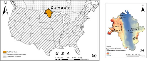
The climate of RRB is classified as humid continental, with warm to hot summers and freezing winters (Peel et al. 2007; Belda et al. 2014). Air temperature ranges between 48 °C in August and −48 °C in January and February (Krenz and Leitch 1993). The average annual precipitation in the basin ranges from approximately 430 mm in the west to more than 673 mm in the east (Group 2015). Usually, 22% of the annual precipitation falls as snow in winter, and the rest falls as rain typically as severe thunderstorms in summer, which may bring up to 7.5 cm per day of rainfall (de Loë 2009). Due to snowmelt and rain on snow, most streamflow occurs in the spring, while heavy rainfall on consecutive days on saturated soil produces runoff in the summer (Mahmood et al. 2017). Nevertheless, the basin relatively flat topography and humid climatic conditions frequently result in substantial floods in the Red River and its tributaries. Flooding mainly occurs in spring and early summer and is more severe during wet periods (Board 2000). Spring floods account for most of the significant historical floods.

In addition to the critical snowmelt streamflow and subsequent flooding, the RRB has other unique watershed characteristics. The basin has numerous regulated reservoirs and dams (Bengtson and Padmanabhan 1999), a flat channel gradient and lack of topographic relief, and the presence of frozen ditches and culverts that temporarily store water during spring runoff (Hu et al. 2006). Furthermore, wetlands remove pollutants and nutrients from water systems allowing lakes, streams, and aquifers to remain clean. Besides, they decrease erosion, lessen flooding, and refill groundwater (Bengtson and Padmanabhan 1999; Juliano and Simonovic, 1999; Simonovic and Juliano, 2001). Many wetlands in the RRB have been lost because of excessive drainage and urbanization (Hearne 2007). The basin is a nearly featureless plain with poorly drained silty and clayey soils. The entire basin is covered with a layer of glacial drift (sand, gravel, and rocks deposited by glaciers). Although groundwater is a vital water source in the RRB, snowmelt runoff provides the majority of the streamflow in the Red River and its tributaries (de Loë 2009).

Three major ecoregions in the RRB are upland, lowland, and escarpment. We define them below (Figure 1b):

1. Upland: Northern Glaciated Plains (Aspen Parkland) make up one-third of the RRB in the west, known as upland, and most of the basin lies in North Dakota (Figure 1b). Flat to gently sloping plains formed of glacial moraine occur throughout the region. There are areas of lacustrine and hummocky to ridged fluvioglacial deposits, with Tertiary and Cretaceous sandstones and shales as the characteristic bedrock. The site has a low density of streams and rivers. Devils Lake basin is a closed basin in the drainage of the Red River in the north, which covers a 9,868 km² area, a large portion of the upland ecoregion. The topographic formation of the Devils Lake Basin is unique due to the great number of shallow depressions of small lakes, ponds, wetlands, moraines, outwash plains, and drumlins (Sethre et al. 2005; Zhang et al. 2009; Shook et al. 2013).

2. Lowland: In the center of the RRB, the lowland region makes up nearly half of the RRB (Figure 1b). It extends down from the basin’s center, enclosing the Red River Valley and orienting north/south along the river. The terrain is extremely flat and has higher elevations only in the south and lower elevations in the north. The river slopes become flat when the tributaries enter the lowlands of the lakebed, with weakly defined watershed boundaries. The area is crisscrossed by the low-density, low-gradient stream, and river networks with typical flooding in late winter and early spring (Galloway 2011).

3. Escarpment: An escarpment between upland and lowland in the western part of the RRB is known as the Manitoba Escarpment (also known as the Pembina Escarpment in North Dakota). The relief is 200 meters with very steep topography in the escarpment (Mahmood et al. 2017). The eastern margin is much less distinct and marked by a gentle topographic rise to late Quaternary glacial deposits.

3. Material and methods

3.1. Data

The could -free water images for spring to summer from GSWD were used to estimate the time series of annual and monthly surface water extent (Pekel et al. 2016). This dataset is free and contains 30 m resolution images for 30 years (1990–2019). The entire archive of the Landsat 5 Thematic Mapper (TM), the Landsat 7 Enhanced Thematic Mapper-plus (ETM+), and the Landsat 8 Operational Land Imager (OLI) orthorectified, top-of-atmosphere reflectance and brightness temperature images (L1T) were used (USGS LANDSAT MISSIONS 2016). Landsats 5, 7, and 8 are in a near-polar orbit with 16-day repeat coverage; two satellites operate at the same time on an 8-day cycle. In our analysis of this data, we quantify the local and regional changes in permanent, seasonal, and total surface water area climatic 30‐year period. The pixels are classified into two categories: permanent water area (PWA) and seasonal water area (SWA). Total water area (TWA) for a year is the addition between PWA and TWA. A pixel is considered a PWA when it is underwater throughout the year while an SWA pixel is inconsistently underwater during a year. Note that the water bodies in NGP are frozen during the winter season (4–5 months depending on the duration of the winter). Surfaces covered with water all year long or for all months with reliable observations are considered to have permanent water. Surfaces that are covered in water seasonally are those that have water for fewer than 12 months of the year or fewer months than the total number of months having valid observations. Total surface water referred to streams, rivers, lakes, reservoirs, and wetlands which can persist all year long or for only part of the year.

The Google Earth Engine (GEE), a computing platform introduced by Google, Inc., has enabled the creation of global-scale data products based on satellite image time series such as the Landsat archive (Gorelick et al. 2017). GGE provides annual (https://developers.google.com/earth-engine/datasets/catalog/JRC_GSW1_3_YearlyHistory) and monthly (https://developers.google.com/earth-engine/datasets/catalog/JRC_GSW1_3_MonthlyHistory) GSWD water history. Water is a highly variable land surface feature and due to the sensitivity of its spectral qualities, a challenging spectral target (at the wavelengths measured by the TM, ETM+, and OLI sensors) to the chlorophyll concentration, total suspended solids, and colored dissolved organic matter load, depths, and bedload material for shallow waters, as well as variations in observation conditions (sun-target sensor geometry, and optical thickness). Pekel et al. (2016) used big data technology systems including expert systems (Kartikeyan et al. 1995; Lu and Weng 2007; Shoshany 2008), visual analytics (Keim et al. 2008), and evidential reasoning to address these issues (Yang and Xu 2002).

The annual GSWD provides data on permanent and seasonal water occurrence over Earth’s continental land area (Pekel et al. 2016). In contrast, the monthly data from Spring to Summer report the occurrence based on the water month of interest. This dataset was funded and published by the European Commission Joint Research Centre (JRC), which also maintains a current archive. Using GEE, we developed algorithms to download annual and monthly water data (from Spring to Summer with limited cloud cover) for the RRB from 1990 to 2019. While annual water data is available for all years with no restrictions due to major cloud cover and Landsat 7 SLC off, the monthly dataset did experience significant cloud cover and Landsat 7 SLC off difficulties. It was often difficult to obtain imagery due to intense and persistent cloud cover during the winter period (Oct-Mar). Therefore, we visually checked all monthly water maps from 1990 to 2019 and created a database of maps with no cloud cover. In this research, we interpret the water maps during April–May period as the spring season water area while the water maps of the July- September period is considered to represent the summer season.

To expand our analysis, precipitation and temperature data and their temporal evolution across the study area are considered to better support our findings and the relation with climate variability. Accessing comprehensive annual precipitation and temperature data can be a challenging task, particularly in the absence of a comprehensive source. In this case, the National Weather Service (NWS) was used to obtain precipitation and temperature data for the study period. To ensure that the data is representative of the region of interest, it is common practice to select specific stations as proxies for the area. To address this issue, the Grand Forks and Fargo stations were chosen as a proxy for the lowland region, while Edmore was selected to represent the upland region. Monthly data was then downloaded for the study period, which was subsequently used to create annual datasets. Considering the lack of data availability during the study period, the data from these three stations are deemed to be representative of the region of interest and is suitable for further analysis and interpretation. To further investigate these trends, we performed an additional Mann-Kendall test to determine the correlation between water surface area, temperature, and precipitation over the four recognized phases.

3.2. Data analyses

We used Singular Spectrum Analyses (SSA) on water areas to decompose major hydroclimatic phases for 30 years in the RRB. SSA is a nonparametric time series analysis method. It can extract as much accurate info as possible by reducing noisy information from time series (Shen et al. 2018; Guo et al. 2019). SSA has evolved into a standard tool for analyzing climate, meteorology, and geophysics time series (Vautard and Ghil 1989; Yiou et al. 1996; Golyandina et al. 2001). The trend, periodic components, and noise components were obtained from SSA. To enhance the application and accuracy of altimeter data, the SSA-denoised waveforms are then reprocessed. Monthly surface water data were used for SSA and to identify the hydroclimatic phases because it dominates the variability in the water budget of a basin. SSA can decompose the monthly surface water data since it has serial dependencies and can be categorized as seasons, years, or decades.

In addition, we utilized the Mann-Kendall trend test on the annual total, permanent, and seasonal water areas as well as precipitation and air temperature in the RRB for the 1990–2019 period. The Mann-Kendall test (Mann 1945) s widely known as a non-parametric test to analyze long-term data sets and detect statistically significant trends. Due to its rank-based procedure with resistance to the influence of extreme values, the method facilitates the trend analysis for variables having skewness (Önöz and Bayazit 2003; Partal and Küçük 2006; Adamowski et al. 2009). The Mann-Kendall test can be utilized to determine whether an increasing or decreasing trend exists (Kendall 1948). In this test, the p-value represents the probability of the error when expecting that the trend differs from zero. The value of Z (absolute) is compared to the standard normal cumulative distribution to determine if there is a trend or not at the selected significance level. A positive or negative value of Z indicates an upward or downward trend.

4. Results

4.1. Annual spatiotemporal variability of surface water area

TWA, which includes both permanent and seasonal water areas (PWA and SWA), increased from 3247 km² in 1990 to 6031 km² in 2019 (Figure 2c). The PWA increased from 2590 to 3635 km², accounting for between 79% to 60% of TWA (Figure 2a). PWA represent large lakes such as Lake Alice, Red Lake, and Devils Lake (Figure 3) while SWAs are considered wetlands in the RRB, and they also show an increase from 656 to 2395 km² over the study period, ranging from 20% to 40% of TWA (Figure 2b). The most noticeable seasonal water area is at the center of the basin near Grand Forks, ND, and Emerson, ND (Figure 3), which is frequently flooded during the springs in wet years. Table 2 shows an upward trend for TWA and PWA for 1990–2019 based upon the Mann-Kendall trend test that is significant at p < 0.05, which is consistent with other studies in the western RRB (e.g. Sethre et al. 2005; Todhunter 2021) and North Great Plain (Vanderhoof et al. 2018). The temporal dynamics of the total water area agree with both permanent and seasonal areas during the 1990–1997 period. However, SWA exhibits noticeable fluctuation in the post-1997 period while the PWA variation is small.

Figure 2. Temporal variation of permanent (lake) water area (a), seasonal (wetland) water area (b), and total (lake + wetland) water area (c) during 1990–2019.

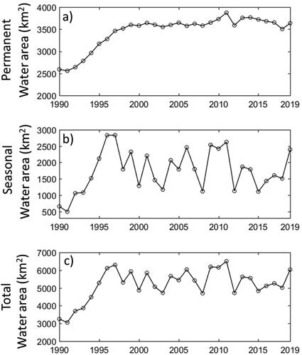
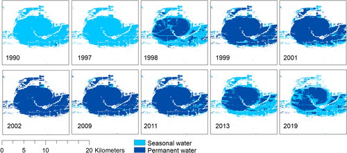
Figure 3. Spatiotemporal variation of seasonal water area in the Red River during 1990–2019. The dark color shows the permanent area with no change. Note that most extreme years in terms of wetness and dryness are shown.

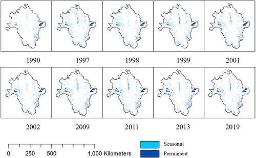
Table 2. Mann-Kendall trend tests with p-value for the annual total, permanent, and seasonal water areas, and monthly (from Spring to Summer) total water areas in the Red River Basin for the 1990–2019, 1990–1999, 2000–2003, 2004–2013 and 2014–2019 periods.

Period		Annual			Monthly
		Permanent	Seasonal	Total	Total
1990–2001	Z	4.18	2.4	2.67	11.14
	p	0.000014	0.008	0.0037	0.00
	Trend	Upward	Upward	Upward	Upward
2002–2005	Z	0.34	0.34	0.34	−0.34
	p	> 0.05	> 0.05	> 0.05	> 0.05
	Trend	No Trend	No Trend	No Trend	No Trend
2006–2013	Z	2.35	0	0.124	2.61
	P	0.009	> 0.05	> 0.05	0.004
	Trend	Upward	No Trend	No Trend	Upward
2014–2019	Z	0.375	0.75	0.376	−3.84
	p	0.012	> 0.05	> 0.05	0.00
	Trend	No Trend	No Trend	No Trend	Downward
1990–2019	Z	1.78	0.75	0.376	12.4
	p	0.032	> 0.05	> 0.05	0.00
	Trend	Upward	No Trend	No Trend	Upward

Figure 3 shows the two most noticeable permanent water bodies; one is the chain of lakes in the Devils Lake area (upland area), and another is large lakes in the Red Lake area (eastern edge of the basin). While all TWA, PWA, and SWA of the Devils Lake Basin have increased substantially, they remain invariable in the Red Lake area. PWA and SWA gained area during the wet years (e.g. 1997, 1998, 2011, and 2013) in the western (around Devils Lake) and southeastern parts of the RRB, which are also situated at higher elevations (>370 m). We also investigated the spatiotemporal variation of PWA and SWA in two test sites. These sites include Devils Lake with about 10,000 km² drainage area in the west (Figure 4) and a large wetland Roseau River with a 30 km² drainage area in the east of the basin (Figure 5). At the beginning of the study period (1990), the Devils Lake Basin had high PWA and SWA, and the PWA is only restricted to Devils Lake (Figure 4). However, the wetting filled up the large depressions north of Devils Lake and converted them into a seasonal water body in 1997 and 1998. The continued wetting in these further added moisture to the system and transformed these seasonal water bodies into permanent water bodies during the 2001–2011 period. These water bodies are known as lake Alice and Irvine. Thus, the Devils Lake Basin experienced two phases of wetting which drastically changed the PWAs; one is the conversion of the empty depression into a seasonal water area during 1990–1999 and another is the transformation of the seasonal water area into a permanent area (2001–2011). The PWA and SWA have declined slightly since 2011.

Figure 4. Spatiotemporal variation of permanent and seasonal water area in Devils Lake during 1990–2019. Most extreme years in terms of wetness and dryness are shown.

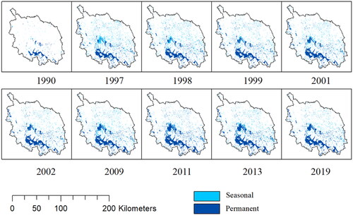
Figure 5. Spatiotemporal variation of permanent and seasonal water area in a small depression in the northeastern Red River during 1990–2019. Most extreme years in terms of wetness and dryness are shown.

In the eastern RRB, the changes in the large water bodies like the Devils Lake Basin of the western RRB were rarely observed. The most noticeable site at which the seasonal-to-permanent water area transformation was observed was in the Roseau River (Figure 5). The area had SWA during the 1990–1997 period. However, the transformation from seasonal to permanent started in 1998 and ended in 1999. Since 1999, the PWA presence was there till 2012. Since 2013, the area started to lose PWA permanent water and gain SWA but did not completely turn into an SWA system.

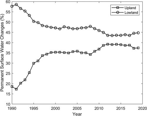
Figure 6 shows the temporal changes of the percent contribution by PWA to RRB in the upland and lowland areas (Figure 1b). In 1990, the PWA contribution in the upland is 18% while it is 58% in the lowland. Over the last three decades, the permanent area contributed from the upland to the entire RRB has increased substantially from 18% to 40%. In upland, two major phases of rapid areal increase are detected, including one in 1990–1998 from 18% to 34% and one in 2007–2013 from 34% to 39%. After 2017, it slightly recessed back to 37% in 2017–2019. In contrast, the PWA contribution has decreased from 58% to 44% in the lowland area. Like the upland area, the recession of the percent contribution by PWA to RRB has two major phases in the lowland area: one in 1990–1998 from 58% to 47% and one in 2007–2013 from 47% to 43%. During 2000–2006 and 2013–2016, the percent contribution of PWA is temporally stable in both upland and lowland areas.

Figure 6. Temporal changes of the percent contribution by permanent water area to Red River Basin PWA in upland (Figure 1b) and lowland areas (Figure 1b). Upland is located on the west of the basin and the elevation varies from 427 to 723 m while the lowland is located in the center and east and the elevation varies from 218 to 370 m.

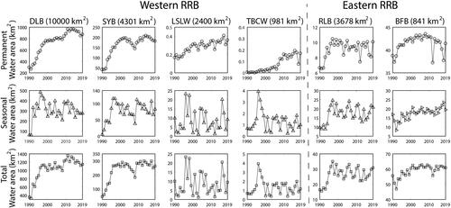
To understand the spatiotemporal variability of TWA, SWA, and PWA, we investigate them in the six headwater basins situated at the different geomorphic units of the RRB (Figure 1b). The six headwater basins are: Devils Lake Basin (DLB), Sheyenne River Basin (SYB), LaSalle Watershed (LSLW), Tobacco Watershed (TBCW), Red Lake River Basin (RLB), and Buffalo Basin (BFB). DLB and SYB are in the upland area, TBCW is in the escarpment area and LSLW and RLB are hosted by the lowland area. BFB is in the highland area of the eastern RRB. The results show in upland, the temporal dynamics of the TWA, PWA, and SWA are consistent with that of the RRB, while the smaller basins such as LSLW and TBCW show different TWA, SWA, and PWA compared to the RRB. In the east of the basin, the temporal changes of TWA, SWA, and PWA of two headwater basins (RL and BFB) are consistent with the RRB.

4.2. Monthly surface water area

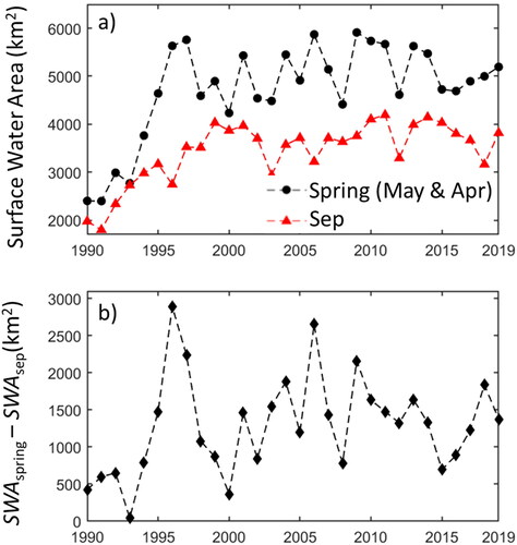
The long-term spring and summer TWA temporal patterns are consistent with that of annual PWA (Figure 8a), showing a steady, progressive increase from 1990 to 1997, and a consistent fluctuation after that year. A consistent seasonal pattern is observed in Figure 8 in which the spring TWA is substantially higher than that in summer. In Figure 8b, the difference between spring and summer TWAs are observed. The difference is substantial in deluge years like 1996 and 1997 and the least difference is observed during the drought year such as 1993 and 2002.

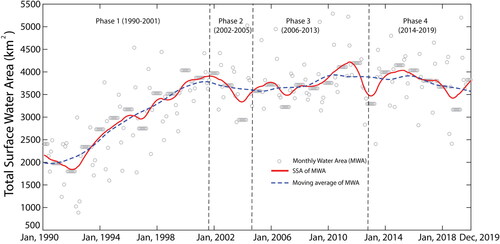
We further analyzed the dynamics of monthly TWA and detected four phases using the single spectrum analysis (Figure 9). The moving average is also used to better identify the phases (Figure 9). The visual inspection of the dynamics of monthly TWA using SSA indicates four phases: phase 1 (1990–2001), phase 2 (2002–2005), phase 3 (2006–2013), and phase 2014–2019). These four phases show an alternation of wetting (TWA increment) and drying (invariant TWA or slight decline in TWA) in the RRB. Phase 1 explicitly shows wetting and a substantial increase of TWA while the acceleration of TWA increment is stalled during phase 2. Phase 3 exhibits a continued increase of TWA after a brief cessation of TWA increment. Finally, phase 4 represents another dry phase during which the TWA has decreased by a moderate amount before a slight rebound in 2019.

5. Discussions

5.1. Annual surface water area

Overall, our results suggest that the TWA has increased in the RRB from 1990 to 2019, which is consistent with the findings of Vanderhoof et al. (2018) and Archambault et al. (2023). While both studies cover only part of the western RRB, our study covers the entire basin. We further analyzed permanent and seasonal water areas from Pekel et al. (2016) and reported the difference in temporal evolution between permanent and seasonal water areas. The direction of changes in permanent water area between 1990 to 2019 in our study agrees well with that of Borja et al. (2020), in which they show that except for some dramatic human‐driven regional drying cases, the world’s surface water systems have expanded, primarily by increased seasonal water from 1985 to 2015. The total, permanent, and seasonal surface water in the RRB have increased in general by ^{2890, 1151, and 1739 km2}, respectively in 30 years (see Table 1). Based on the map net change in Borja et al. (2020) for surface water area over regional hydrological catchments between 1985–2000 and 2001–2015, permanent water in the RRB gains less than 2000 km² area, and surface and total water gain 2000 to 5000 km² area (Borja et al. 2020). The total surface water includes a major impact on the pattern of seasonal water changing and a relatively small increase in permanent water changing. A comparison of estimated changes in long-term permanent water cover by Borja et al. (2020), between 1985 and 2015, shows disagreement in the direction of change that is like that between part 1 and Donchyts et al. (2016). Especially, Borja et al. (2020) study part 2 period, between 1985–2005, and 2013–2015, and Donchyts et al. (2016) are consistent in estimating an average net land area gain (permanent water loss) from the long 15-year period 1985–2005 to the short 3-year period 2013–2015, even though change magnitudes differ between these two studies (Donchyts et al. 2016). PWA is primarily determined by the amount of precipitation the wetland receives and the amount of water that flows into and out of the wetland. This means that areas that receive more precipitation or have greater streamflow will have a larger permanent water area. In contrast, SWA is affected by how water interacts with the wetland and groundwater, as well as the rate of open water evaporation. The interaction between these factors determines whether the wetland will have seasonal water, and how long it will stay submerged during the year. Our findings add new knowledge by showing the more gradual and consistent increment of PWA and highly variable temporal response by SWAs.

Table 1. Seasonal, permanent, and total wetlands’ surface water area assessed on annual surveys in the Red River Basin, 1990–2019.

Year	Surface water Area (km^2)
	Seasonal	Permanent	Total
1990	656.9	2590.8	3247.7
1991	494.9	2557.5	3052.4
1992	1061.2	2640.7	3701.9
1993	1080.9	2782.7	3863.5
1994	1520.4	2962.2	4482.6
1995	2116.8	3169.4	5286.2
1996	2833.1	3277.7	6110.8
1997	2835.2	3462.8	6298.1
1998	1791.8	3517.3	5309.1
1999	2327.0	3599.5	5926.5
2000	1287.4	3581.8	4869.2
2001	2207.1	3642.6	5849.6
2002	1458.8	3601.2	5060.0
2003	1171.9	3550.1	4722.0
2004	2068.1	3597.9	5666.0
2005	1791.8	3647.9	5439.8
2006	2460.7	3575.7	6036.4
2007	1795.6	3623.8	5419.4
2008	1117.8	3580.7	4698.5
2009	2538.8	3650.5	6189.3
2010	2422.5	3729.7	6152.2
2011	2626.9	3874.6	6501.6
2012	1126.9	3588.6	4715.5
2013	1869.6	3759.0	5628.6
2014	1788.1	3766.0	5554.1
2015	1109.4	3721.8	4831.2
2016	1433.6	3681.1	5114.8
2017	1606.2	3651.5	5257.8
2018	1509.6	3503.9	5013.5
2019	2395.8	3635.4	6031.2

The spatial analyses of the PWA and SWA revealed additional new knowledge in the context of the RRB. Our analyses deciphered a noticeable seasonal water area which is located at the central part (Grand Forks, ND to Emerson, ND) of the RRB (Figure 3). During the wet years (e.g. 2009, 2011, and 2013), this area is flooded during the spring season due to flat topography and downstream ice-jam in Red River and Lake Winnipeg (Figure 3). In addition to detecting a sensitive area to seasonal water inundation, we further detected two most noticeable permanent water bodies with the diminishing influence of SWA during the study period; one is the chain of lakes in the Devils Lake Basin area (west of RRB in upland, Figure 4) and a large wetland Roseau River, 30 km² in the eastern RRB (Figure 5). Annual precipitation onto the lake surface (P_L) is 421.6 mm from 1907 to 1980, while P_L is 506.0 mm from 1981 to 2011 which shows the Devils Lake Basin experienced high precipitation regime since 1980 (Todhunter 2016) resulting in filling up potholes and depression and basin storage. However, the surface water area has started to respond since mid-1990, as Figure 4 shows the emergence of SWA in 1997. The continued wetting converted the SWA to PWA during the study period. The diminishing influence of SWAs indicates that the Devils Lake Basin system transitioned from low streamflow and high evaporation system to high streamflow and low evaporation system while annual precipitation remains high and invariable during the study period (Archambault et al. 2023). While another wetland is small in area (30 km²) relative to chains of lakes the Devils Lake Basin area shows remarkable transition between SWA and PWA during the study period (Figure 5). This wetland also has demonstrated that the smaller water body is more susceptible and highly to any local or regional climatic fluctuations.

Our study also indicates that the western upland geomorphic unit of the RRB has higher PWA than the lowland geomorphic unit located at the central part and partly in the eastern RRB. This comparison between upland and lowland is also consistent with the hydro lake database by Messager et al. (2016). According to the upland area PWA contribution to the RRB, PWA increased substantially, while the lowland PWA contribution to the RRB decreased. The percent of PWA contribution in 1990, 1999, 2009, and 2019 are 18, 35, 36, and 37% for the upland, while it is 58, 47, 47, and 45% for the lowland. Note that the PWA of upland RRB has increased at a much faster rate than the lowland. The upland’s PWA has increased at a rate of 40 km²/year while the rate is only 4 km²/year in the lowland area. Rapid filling of potholes and depressions in the upland area during the 1990–1998 period has generated many permanent water bodies, improved wetland connectivity, and increased contributing areas resulting in substantial streamflow in the major tributaries (e.g. Sheyenne River, Mauvais Coulee) of Red River draining from the upland area. Similar phenomena are also observed during the 2009–2013 period resulting in massive streamflow and regional flooding in 2009, 2011, and 2013. We think the lowland permanent area is already filled at its maximum capacity at the onset of the study period. Moreover, compared to uplands, lowlands have a shallower water table due to lower elevation, flatter topography, and groundwater convergence from uplands, allowing for higher evapotranspiration and leaf area index in many places (Subin et al. 2014). It can be concluded that the lowland is already filled up, for any flood in the future, the upland would be responsible and will lead the water to the lowland part which is in a flatter area.

The western RRB has a low density of streams and rivers but high densities of temporary and seasonal wetlands. The topographic formation of the RRB is of glacial origin and is unique due to the great number of shallow depressions of small lakes, ponds, wetlands, moraines, outwash plains, and drumlins (Sethre et al. 2005; Zhang et al. 2009; Shook et al. 2013). As can be seen in Figure 7, the permanent surface water has a big portion of the total water in both Devils Lake Basin and SYB which are from the upland area. In contrast, escarpment watersheds (TBCW and LSLW) have a low amount of PWA as the steeper slope of the channel causes rapid draining of wetlands and water bodies. The RLB has a low PWA due to the extensive development of drainage ditches at both headwater and downstream RLB (Stoner et al. 1993).

Figure 7. Temporal variation of permanent (lake) water area, seasonal (wetland) water area, and total water area during 1990–2019 in the six headwater basins. Note that the first four columns from the left represent the subbasins located in the western Red River while the rest of the two columns from the right represent the subbasins in the eastern Red River Basin. The first two columns from the left are Devils Lake Basin and SYB which are in the upland area.

5.2. Monthly water area

The spring TWA strongly responded during the 1990–1997 wetting period, showing a significant increase across the RRB, but then subdued and fluctuated little for the rest of the study period (1998–2019) (Figure 8a). The summer TWA also responded to initial wetting and the TWA increment was observed till 2000. Since 2000, summer season TWA remained slightly variable (between 3000 and 4000 km²) partly due to the consumption of summer rainfall by evapotranspiration (Figure 8a). The difference between the spring and summer TWAs (diff_TWA) shows an interesting pattern of temporal changes (Figure 8b). The spring TWA is dominated by snowmelt runoff, frozen soil infiltration, rain on snow, fill-spill hydrology, and variable contributing areas while the summer TWA depends on summer rainfall, the timing of the rainfall, evapotranspiration, open water evaporation, cloud-cover and images for spring to summer from GSWD days. Hence, the diff_TWA is the result of the competition between winter snow accumulations, spring, and summer processes. The high diff_TWA is observed during 1996, 1997, and 2006 as both years have contrasting spring (wet) and summer (dry) seasons. However, other years having wet springs like 2009, 2011, and 2013 have moderate diff_TWA as the late summer rainfall is responsible for the rebound of the TWA.

Figure 8. (a) Temporal dynamics of spring (Apr, May) and summer (Sep) monthly total water area (cloud-free and available data). (b) Temporal dynamics of the difference of total water area between spring and summer.

The visual inspection of the temporal dynamics monthly TWA using SSA indicates four phases: phase 1 (1990–2001), phase 2 (2002–2005), phase 3 (2006–2013), and phase (2014–2019). The Mann-Kendall tests are conducted on the SSA of monthly TWAs (Table 2) and the test results show an upward trend for phase 1 and phase 3, no trend for phase 2, and a downward trend for phase 4. These phases are consistent with regional hydroclimatology of the RRB that phase 1 and phase 3 are wetting periods, phase 2 is part of prairie drought and phase 4 is part of the recent dry condition. Phase 1 (1990–2001) exhibits wetting in which the RRB consistently received noticeable snowfall (with subsequent snow accumulation and melt) and rainfall resulting in the expansion of existing lakes and the creation of new lakes and smaller water bodies (Figures 3–5). The monthly TWA shows a steady, large increase with time. The phase 2 (2002–2005) period experienced sustained high TWA and PWA due to memory effects inherited from phase 1 (1990–2001). The short dry period from 2002 to 2005 was not long enough to have a significant influence on lakes so monthly TWA remained stable (Figure 9). Due to the drought condition during phase 2, the monthly TWA experienced minor fluctuations with no significant trend in the Mann-Kendall test statistic (Table 2). SWA started to decline in the summer of 1997 and depletion continued through 2003 due to persistent dry summer conditions. After this short prairie drought (phase 2), the RRB experienced remarkable wetting during the 2006–2013 period (phase 3 in Figure 9). The wet condition did not fully kick in until 2010, although precipitation started to increase in the fall of 2006. Table 2 shows an upward trend with 95% confidence. The phase 4 (2014–2019) period shows a decrease in monthly TWA, indicating a drying period in the RRB (Figure 9). Table 2 shows downward trends for TWA, PWA, and SWA at the 95% confidence level.

Figure 9. Monthly TWA, singular spectrum analyses (SSA), and moving average of monthly TWA during the study period.

Precipitation and temperature data and their temporal evolution across the study area are considered to further investigate how water area relates to climate variability. We performed an additional Mann-Kendall test to determine the correlation between water surface area, temperature, and precipitation over the four recognized phases. Tables 3 and 4 show the Mann-Kendall test results for temperature and precipitation respectively, for the study period. Overall, there is no trend for temperature and precipitation during the study period except an upward trend in precipitation at the Upland station. In the first phase, the excessively wet period from 1990 to 2001, there is an upward trend in precipitation in both upland and lowland stations (Table 4). However, there is no trend in temperature during phase 1 in all stations. We further investigate temperature fluctuations during phase 1 and detect a period (1990–1996, Z = −3.0, p = 0.001) of cooling and wetting at Edmore (Upland) and Fargo (headwater lowland) station. Annual Average temperature has dropped by 7 F during this period. While the wetting continues during the latter part of phase 1, no trend is observed for temperature in Edmore and Fargo stations and an upward trend in Grand Forks station. We believe the combination of cooling and wetting during the 1990–1996 period trigger a substantial increase in PWA, SWA and monthly water area. We believe that, during 1990–1996 period, wetting has added moisture to RRB system and cooling has triggered lack of evaporation and sublimation loss, extended winter and snow cover, and subsequent melt runoff to the RRB system.

Table 3. Mann-Kendall trend tests with a p-value for temperature in the Red River Basin for the 1990–2019, 1990–1999, 2000–2003, 2004–2013, and 2014–2019 periods.

Period		Lowland Upland
		Grand Forks	Fargo	Edmore
1990–2001	Z	−1.029	−0.206	0.069
	p	> 0.05	> 0.05	> 0.05
	Trend	No Trend	No Trend	No Trend
2002–2005	Z	0	−0.245	1.02
	p	> 0.05	> 0.05	> 0.05
	Trend	No Trend	No Trend	No Trend
2006–2013	Z	−0.124	0	−0.253
	P	>0.05	>0.05	–
	Trend	No Trend	No Trend	No Trend
2014–2019	Z	−0.75	−0.75	0.75
	p	>0.05	>0.05	>0.05
	Trend	No Trend	No Trend	No Trend
1990–2019	Z	−0.214	0.304	−0.174
	p	>0.05	>0.05	>0.05
	Trend	No Trend	No Trend	No Trend

Table 4. Mann-Kendall trend tests with a p-value for precipitation in the Red River Basin for the 1990–2019, 1990–1999, 2000–2003, 20,04–2013, and 2014–2019 periods.

Period		Lowland Upland
		Grand Forks	Fargo	Edmore & Others
1990–2001	Z	2.5	1.787	2.336
	p	0.006	0.037	0.0098
	Trend	Upward	Upward	Upward
2002–2005	Z	0	1.225	1.019
	p	>0.05	>0.05	>0.05
	Trend	No Trend	No Trend	No Trend
2006–2013	Z	−0.124	0.124	1.361
	P	>0.05	>0.05	>0.05
	Trend	No Trend	No Trend	No Trend
2014–2019	Z	0.75	1.127	−0.34
	p	>0.05	>0.05	>0.05
	Trend	No Trend	No Trend	No Trend
1990–2019	Z	1.265	0.624	2.271
	p	>0.05	>0.05	0.0034
	Trend	No Trend	No Trend	Upward

Over the study period, an analysis of surface water area during a long-term drought-to-deluge cycle showed a net spike in temporal, permanent, and seasonal water areas in RRB. Figure 10 summarizes the details of such changes and shows the spatial distribution of the transitions between permanent water, seasonal water, and bare land and the net land cover changes over the last three decades. The RRB-wide transition from bare land to permanent (170 km²) and seasonal (1851 km²) water area is observed during the 1990–2001 period. In contrast, changes are minimal during the following stable period (2002–2005). In the recent wetting period of 2006–2013, a net gain of 354 km² in permanent water from seasonal and bare land is observed while 434 km² changes from bare land to the seasonal water area. These changes are heavily concentrated around the west of the basin. Finally, during the recent drying period (2014–2018), a significant loss (462.3 km²) of seasonal water area to bare land occurred. Table 5 summarized the changes in permanent and seasonal water area and bare land (non-water area) during the period of each phase.

Figure 10. Change between permanent and seasonal water area and bare land (non-water area) during each phase and study period.

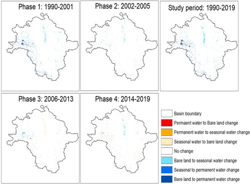
Table 5. Change in permanent and seasonal water area (km²) and bare land (non-water area, km²) during each phase.

Change	1990–01	2002–05	2006–13	2014–19	1990–2019
Permanent water to bare land	1	8	9	63	5
Permanent water to seasonal water	17	87	52	164	31
Seasonal water to bare land	141	355	812	462	143
No change	113467	115236	114889	114911	113309
Bare land to seasonal water	1851	722	435	857	1876
Seasonal to permanent water	170	124	219	91	169
Bare land to permanent water	903	18	135	2	1018

6. Summary and conclusion

This study explores the spatiotemporal variability of surface water area in the RRB during the 1990–2019 period. We provided a more critical assessment of the surface water area variation in RRB and identified surface water area response to drought periods. In this study, we explored permanent, seasonal water areas using the Global Surface Water Dataset (GSWD) with a 30 m resolution. We found that the overall trends for all total, permanent, and seasonal water areas show an increasing trend over the study period. TWA, PWA, and SWA have an increasing trend during the 1990–1997 period. Such increasing trends of TWA, PWA, and SWA are partly due to cooling and wetting during the 1990–1996 period. After 1997, the seasonal water area exhibits noticeable fluctuations while the permanent water variation is slight.

From 1990 to 1998, large depressions in Devils Lake, which is the largest watershed in upland, were filled up and converted into seasonal water bodies. Then, these seasonal water bodies were converted to permanent water bodies from 2001 to 2011. We conclude that since these transitions happened, the upland became representative of the permanent water area in the Red River. In contrast, the transformation from seasonal to permanent water happened in 1998 and 1999 for the lowland. However, PWA decreased after 2013 and partially converted to SWA again.

We detected four phases of variation in the surface water area, including phase 1, a wet period with a substantial increase in TWA from 1990 to 2001; phase 2 from 2002 to 2005; phase 3 from 2006 to 2013 with the acceleration of TWA increment stalled SWA; and phase 4, a dry period with a decrease in TWA from 2014 to 2019. The RRB-wide transition from bare land to permanent (170 km²) and seasonal (1851 km²) water area is observed during the 1990–2001 period. In contrast, during the following stable period (2002–2005), changes are minimal. In the recent wetting period of 2006–2013, a net gain of 354 km² in permanent water from seasonal and bare land is observed while 434 km² changes from bare land to the seasonal water area. These changes are heavily concentrated around the west of the basin. Finally, during the recent drying period (2014–2018), a significant loss (462.3 km²) of seasonal water area to bare land occurred.

The PWA of upland RRB has been increased at a much faster rate than the lowland. As a result, massive and more frequent flooding has been observed in the basins of the upland areas such as Devils Lake Basin. The frequent and massive flooding in the upland areas has raised concerns for the lowland flooding as the water drains from upland to lowland via escarpment. The surface water area variations and identified phases have significant implications for anticipating future lake and wetland area response in the RRB. Bonsal et al. (2013) predicted frequent occurrence of drought with high severity and persistent multi-year drought in the southern prairies. The surface water area response to expected dry conditions in the future or wet-to-dry transition can be linked with phase 2 and phase 4 monthly TWA response. Further, the multi-year dry period (2002–2004) can be comparable to phase 2. This study can be used for preparedness for the dramatic and inevitable extreme surface water area response (flooding) and eutrophication in the Red River.

Our findings also have implications on the level of nutrient concentration in lakes and wetlands of the RRB, as these water bodies are vulnerable to eutrophication (Jeannotte et al. 2020). The increase in surface water area can dilute the nutrient concentration assuming a limited supply from the catchment. In addition, the geochemical environment of some water bodies triggers denitrification. However, during hydrologically extreme events, large nutrient loads can enter the lakes and wetlands of the RRB. The use of water body determination indices such as NDWI, MNDWI, and AWEI in the Red River Basin will be investigated in our future studies. These indices will be employed to comprehensively map and monitor the spatiotemporal dynamics of water bodies in the region, as well as to estimate various water quality parameters. Our goal is to provide valuable insights into the use of remote sensing data for effective water resource management and hydrological studies in the Red River Basin.

Data availability statement

Raw data were generated at the University of North Dakota. Derived data supporting the findings of this study are available from the corresponding author on request.

Disclosure statement

No potential conflict of interest was reported by the authors.

References

- Adamowski K, Prokoph A, Adamowski J. 2009. Development of a new method of wavelet aided trend detection and estimation. Hydrol Process. 23(18):2686–2696.
- Archambault AL, Mahmood TH, Todhunter PE, Korom SF. 2023. Remotely sensed surface water variations during drought and deluge conditions in a Northern Great Plains terminal lake basin. J Hydrol Reg Stud. 47:101392.
- Atashi V, Gorji HT, Shahabi SM, Kardan R, Lim YH. 2022. Water level forecasting using deep learning time-series analysis: a case study of Red River of the North. Water. 14(12):1971.
- Belda M, Holtanová E, Halenka T, Kalvová J. 2014. Climate classification revisited: from Köppen to Trewartha. Clim Res. 59(1):1–13.
- Bengtson ML, Padmanabhan G. 1999. A hydrologic model for assessing the influence of wetlands on flood hydrographs in the Red River Basin: development and application. Fargo (ND): North Dakota Water Resources Research Institute, North Dakota State University.
- Blais E-L, Greshuk J, Stadnyk T. 2016. The 2011 flood event in the Assiniboine River Basin: causes, assessment and damages. Can Water Resour J/Revue Canadienne Des Ressources Hydriques. 41(1–2):74–84.
- Board RRB. 2000. Inventory team report: hydrology. Moorhead (MN): Red River Basin Board .
- Bonsal BR, Aider R, Gachon P, Lapp S. 2013. An assessment of Canadian prairie drought: past, present, and future. Clim Dyn. 41(2):501–516.
- Bonsal BR, Wheaton EE, Chipanshi AC, Lin C, Sauchyn DJ, Wen L. 2011. Drought research in Canada: a review. Atmos Ocean. 49(4):303–319.
- Borja S, Kalantari Z, Destouni G. 2020. Global wetting by seasonal surface water over the last decades. Earth’s Future. 8(3):e2019EF001449.
- Bullock A, Acreman M. 2003. The role of wetlands in the hydrological cycle. Hydrol Earth Syst Sci. 7(3):358–389.
- de Loë R. 2009. Sharing the waters of the Red River basin: a review of options for transboundary water governance. Guelph, Canada: Prepared for International Red River Board, International Joint Commission. Rob de loë Consulting Services. http://www.ijc.org/files/publications/Sharing%20the%20Waters%20of%20the%20Red%20River%20Basin.pdf.
- Donchyts G, Baart F, Winsemius H, Gorelick N, Kwadijk J, Van De Giesen N. 2016. Earth’s surface water change over the past 30 years. Nat Clim Change. 6(9):810–813.
- Dumanski S, Pomeroy JW, Westbrook CJ. 2015. Hydrological regime changes in a Canadian Prairie basin. Hydrol Process. 29(18):3893–3904.
- Galloway JM. 2011. Simulation of the effects of the Devils Lake State Outlet on hydrodynamics and water quality in Lake Ashtabula, North Dakota, 2006–10. U. S. Geological Survey, Bismarck, ND.
- Golyandina N, Nekrutkin V, Zhigljavsky AA. 2001. Analysis of time series structure: SSA and related techniques. New York (USA): CRC press.
- Gorelick N, Hancher M, Dixon M, Ilyushchenko S, Thau D, Moore R. 2017. Google Earth Engine: planetary-scale geospatial analysis for everyone. Remote Sens Environ. 202:18–27.
- Group PC. 2015. 30-year normals. Corvallis (OR): Oregon State University.
- Gulbin S. 2017. Impact of wetlands loss on the long-term flood risks of Devils Lake in a changing climate. Grand Forks (ND): The University of North Dakota.
- Guo J, Shi K, Liu X, Sun Y, Li W, Kong Q. 2019. Singular spectrum analysis of ionospheric anomalies preceding great earthquakes: case studies of Kaikoura and Fukushima earthquakes. J Geodyn. 124:1–13.
- Harden TM, O'Connor JE, Driscoll DG. 2015. Late holocene flood probabilities in the black hills, South Dakota with emphasis on the medieval climate anomaly. Catena. 130:62–68.
- Hearne RR. 2007. Evolving water management institutions in the Red River Basin. Environ Manage. 40(6):842–852.
- Hu HH, Kreymborg LR, Doeing BJ, Baron KS, Jutila SA. 2006. Gridded snowmelt and rainfall-runoff CWMS hydrologic modeling of the Red River of the North Basin. J Hydrol Eng. 11(2):91–100.
- Jeannotte TL, Mahmood TH, Vandeberg GS, Matheney RK, Hou X, Van Hoy DF. 2020. Impacts of cold region hydroclimatic variability on phosphorus exports: insights from concentration-discharge relationship. J Hydrol. 591:125312.
- Juliano K, Simonovic SP. 1999. The impact of wetlands on flood control in the Red River Valley of Manitoba. Final Report to International Joint Commission. International Joint Commission. Washington, DC.
- Kartikeyan B, Majumder KL, Dasgupta A. 1995. An expert system for land cover classification. IEEE Trans Geosci Remote Sensing. 33(1):58–66.
- Keim DA, Mansmann F, Schneidewind J, Thomas J, Ziegler H. 2008. Visual analytics: Scope and challenges. Springer Berlin Heidelberg; p. 76–90.
- Kelly SA, Takbiri Z, Belmont P, Foufoula-Georgiou E. 2017. Human amplified changes in precipitation–runoff patterns in large river basins of the Midwestern United States. Hydrol Earth Syst Sci. 21(10):5065–5088.
- Kendall MG. 1948. Rank correlation methods.
- Kharel G, Zheng H, Kirilenko A. 2016. Can land-use change mitigate long-term flood risks in the Prairie Pothole Region? The case of Devils Lake, North Dakota, USA. Reg Environ Change. 16(8):2443–2456.
- Kolmakova M. 2012. Hydrological and climatic variability in the river basins of the West Siberian Plain (from meteorological stations, model reanalysis and satellite altimetry data). Toulouse: Université Paul Sabatier-Toulouse III].
- Krenz G, Leitch J. 1993. A river runs north: managing an international river. Bismarck (ND): Red River Water Resources Council.
- Liu G, Schwartz FW, Tseng KH, Shum C. 2015. Discharge and water‐depth estimates for ungauged rivers: combining hydrologic, hydraulic, and inverse modeling with stage and water‐area measurements from satellites. Water Resour Res. 51(8):6017–6035.
- Lu D, Weng Q. 2007. A survey of image classification methods and techniques for improving classification performance. Int J Remote Sens. 28(5):823–870.
- Mahmood TH, Pomeroy JW, Wheater HS, Baulch HM. 2017. Hydrological responses to climatic variability in a cold agricultural region. Hydrol Process. 31(4):854–870.
- Mann HB. 1945. Nonparametric tests against trend. Econometrica: J Econ Soc. 13(3):245–259.
- Messager ML, Lehner B, Grill G, Nedeva I, Schmitt O. 2016. Estimating the volume and age of water stored in global lakes using a geo-statistical approach. Nat Commun. 7(1):13603.
- Negm A, Abdrakhimova P, Hayashi M, Rasouli K. 2021. Effects of climate change on depression‐focused groundwater recharge in the Canadian Prairies. Vadose Zone J. 20(5):e20153.
- Önöz B, Bayazit M. 2003. The power of statistical tests for trend detection. Turk J Eng Environ Sci. 27(4):247–251.
- Partal T, Küçük M. 2006. Long-term trend analysis using discrete wavelet components of annual precipitations measurements in Marmara region (Turkey). Phys Chem Earth Parts A/B/C. 31(18):1189–1200.
- Peel MC, Finlayson BL, McMahon TA. 2007. Updated world map of the Köppen-Geiger climate classification. Hydrol Earth Syst Sci. 11(5):1633–1644.
- Pekel J-F, Cottam A, Gorelick N, Belward AS. 2016. High-resolution mapping of global surface water and its long-term changes. Nature. 540(7633):418–422.
- Rasouli K, Scharold K, Mahmood TH, Glenn NF, Marks D. 2020. Linking hydrological variations at local scales to regional climate teleconnection patterns. Hydrol Processes. 34(26):5624–5641.
- Robarts RD, Zhulidov AV, Pavlov DF. 2013. The state of knowledge about wetlands and their future under aspects of global climate change: the situation in Russia. Aquat Sci. 75(1):27–38.
- Rodell M, Famiglietti JS, Wiese DN, Reager J, Beaudoing HK, Landerer FW, Lo M-H. 2018. Emerging trends in global freshwater availability. Nature. 557(7707):651–659.
- Rogers P, Kaiser J, Kellenbenz D, Ewens M. 2013. A comparative hydrometeorological analysis of the 2009, 2010, and 2011 Red River of the North Basin Spring floods. Grand Forks (ND): National Weather Service, Central Region Technical Attachment(13-03).
- Sethre PR, Rundquist BC, Todhunter PE. 2005. Remote detection of prairie pothole ponds in the Devils Lake Basin, North Dakota. GISci Remote Sens. 42(4):277–296.
- Shaw DA, Vanderkamp G, Conly FM, Pietroniro A, Martz L. 2012. The fill–spill hydrology of prairie wetland complexes during drought and deluge. Hydrol Process. 26(20):3147–3156.
- Shen Y, Guo J, Liu X, Kong Q, Guo L, Li W. 2018. Long-term prediction of polar motion using a combined SSA and ARMA model. J Geod. 92(3):333–343.
- Shook K, Pomeroy JW, Spence C, Boychuk L. 2013. Storage dynamics simulations in prairie wetland hydrology models: evaluation and parameterization. Hydrol Process. 27(13):1875–1889.
- Shoshany M. 2008. Knowledge based expert systems in remote sensing tasks: quantifying gain from intelligent inference. Int Soc Photogramm Remote Sens Arch. 37:1085–1088.
- Simonovic S, Juliano K. 2001. The role of wetlands during low frequency flooding events in the Red River basin. Can Water Resour J. 26(3):377–397.
- Stadnyk T, Dow K, Wazney L, Blais E-L. 2016. The 2011 flood event in the Red River Basin: causes, assessment and damages. Can Water Resour J/Revue Canadienne Des Ressources Hydriques. 41(1–2):65–73.
- Subin Z, Milly PC, Sulman B, Malyshev S, Shevliakova E. 2014. Resolving terrestrial ecosystem processes along a subgrid topographic gradient for an earth-system model. Hydrol Earth Syst Sci Discuss. 11(7):8443–8492.
- Todhunter PE. 2016. Mean hydroclimatic and hydrological conditions during two climatic modes in the Devils Lake Basin, North Dakota (USA). Lakes Reservoirs. 21(4):338–350.
- Todhunter P. 2021. Hydrological basis of the Devils Lake, North Dakota USA, terminal lake flood disaster. Nat Hazards. 106(3):2797–2824.
- Todhunter PE, Fietzek-DeVries R. 2016. Natural hydroclimatic forcing of historical lake volume fluctuations at Devils Lake, North Dakota (USA). Nat Hazards. 81(3):1515–1532.
- Stoner JD, Lorenz DL, Wiche GJ, Goldstein RM. 1993. Red River of the North Basin, Minnesota, North Dakota, And South Dakota 1. J Am Water Resources Assoc. 29(4):575–615.
- USGS LANDSAT MISSIONS. 2016. Landsat 8 data users handbook. Reston (VA): United States Geological Survey.
- Van Hoy DF, Mahmood TH, Todhunter PE, Jeannotte TL. 2020. Mechanisms of cold region hydrologic change to recent wetting in a northern glaciated landscape. Water Resour Res. 567:e2019WR026932.
- Vanderhoof MK, Distler HE, Lang MW, Alexander LC. 2018. The influence of data characteristics on detecting wetland/stream surface-water connections in the Delmarva Peninsula, Maryland and Delaware. Wetl Ecol Manag. 26(1):63–86.
- Vautard R, Ghil M. 1989. Singular spectrum analysis in nonlinear dynamics, with applications to paleoclimatic time series. Physica D. 35(3):395–424.
- Wang S, Russell HA. 2016. Forecasting snowmelt-induced flooding using GRACE satellite data: a case study for the Red River watershed. Can J Remote Sens. 42(3):203–213.
- Yang J-B, Xu D-L. 2002. On the evidential reasoning algorithm for multiple attribute decision analysis under uncertainty. IEEE Trans Syst Man Cybern-Part A: Syst Hum. 32(3):289–304.
- Yiou P, Baert E, Loutre M-F. 1996. Spectral analysis of climate data. Surv Geophys. 17(6):619–663.
- Zhang B, Schwartz FW, Liu G. 2009. Systematics in the size structure of prairie pothole lakes through drought and deluge. Water Resour Res. 45(4):W04421.