Bayesian logistic regression analysis for spatial patterns of inter-seasonal drought persistence

Abstract

Drought is one of the disastrous natural hazards with complex seasonal and spatial patterns. Understanding the spatial patterns of drought and predicting the likelihood of inter-seasonal drought persistence can provide substantial operational guidelines for water resource management and agricultural production. This study examines drought persistence by identifying the spatial patterns of seasonal drought frequency and inter-seasonal drought persistence in the northeastern region of Pakistan. The Standardized Precipitation Index (SPI) with a three-month time scale is used to examine meteorological drought. Furthermore, Bayesian logistic regression is used to calculate the probability and odds ratios of drought occurrence in the current season, given the previous season’s SPI values. For instance, at Balakot station, for the summer-to-autumn season, the value of the odds ratio is significant (6.78). It shows that one unit increase in SPI of the summer season will cause a 5.78 times to increase in odds of autumn drought occurrence. The average drought frequency varies from 37.3 to 89.1%, whereas the average inter-seasonal drought persistence varies from 21.9 to 91.7% in the study region. Results indicate that some areas in the study region, like Kakul and Garhi Dupatta, are more prone to drought and vulnerable to inter-seasonal drought persistence. Furthermore, the Bayesian logistic regression results reveal a negative relationship between spring drought occurrence and winter SPI, demonstrating that the overall study region is more prone to winter-to-spring drought persistence and less vulnerable to summer-to-autumn drought persistence. Overall study has concluded that the region’s seasonal drought forecast is challenging due to uncertain drought persistence patterns. However, the Bayesian logistic regression model provides more accurate and precise regional seasonal drought forecasts. The outcome of the present study provides scientific evidence to develop early warning systems and manage seasonal crops in Pakistan.

Keywords:

• Bayesian logistic regression
• drought persistence
• Gibbs sampling
• inter-seasonal
• standardized precipitation index

1. Introduction

Drought is the least understood and one of the costliest natural hazards virtually occurs in all geographical areas (He et al. 2013). It is the persistent period of water scarcity caused by less than-normal precipitation in the region (Slette et al. 2019). Usually, drought can be classified into four categories, including meteorological, hydrological, agricultural and socio-economic drought. Still, the basic theme in each drought classification is the concept of water deficit (Mishra and Singh 2010). The drought negatively affects water resources, the local environment, agriculture, society and terrestrial biomes (Wilhite and Glantz, 1985; AghaKouchak et al. 2021). The evolution, termination period and severity of drought are complex and cannot be predicted easily because drought is nonstructural (Sheffield and Wood 2008; Wang et al. 2011; Shah and Mishra 2020). Drought mitigation requires meticulous water resource planning to reduce the drought impacts and to predict the onset of drought (Bandyopadhyay et al. 2020; Katipoğlu 2023). Drought is a creeping phenomenon; it develops in slow spatial and temporal patterns and can persist from one season to another, even during wet periods (Sönmez et al. 2005). Studies suggest that drought projections increase due to global warming and precipitation patterns may change shortly in several parts of the world (Chiew et al. 2011; Wang et al. 2015; Dikshit et al. 2022). Furthermore, Drought persistence causes significant repercussions on the hydrosphere across the globe (Naumann et al. 2018; Wei et al. 2022). It puts massive pressure on freshwater resources, which causes a devastating impact on the linked ecosystem and socio-economic sector (Lorenzo-Lacruz et al. 2010; Luo et al. 2020; Katipoğlu 2022b). Recurrent drought episodes have severely affected the global climate, including in Pakistan.

Pakistan is predominantly categorized as an arid region, and much of the economy is based on agriculture. It contributes 23.13% to Gross Domestic Product (GDP) and absorbs almost 42.3% of the country’s labour force. According to World Bank, the total agricultural land in Pakistan irrigated from controlled water reservoirs was 53.22% in 2018. Pakistan has the largest contiguous irrigation system in the world, the Indus Basin Irrigation System (IBIS). In 1998 the worst drought-hit most parts of the country, and it prolonged till 2002, causing negative agriculture growth (Rahman et al. 2021). The agriculture sector is particularly vulnerable to potential drought events (Khan and Atta-ur-Rahman, 2011; Benevolenza and DeRigne 2019; Kuwayama et al. 2019). Some areas of Pakistan are more prone to persistent droughts than others because the region’s hydro-climatology is diverse (Ullah et al. 2019; Adnan and Ullah 2020).

In general, drought is monitored and quantified by standardized drought indices. Numerous drought indices have been introduced in the literature to assess and monitor drought severity, duration and frequency (Spinoni et al. 2014; AghaKouchak et al. 2015). Standardized Precipitation Index (SPI) (Mckee et al. 1993) and Palmer Drought Severity Index (PDSI) (Palmer 1965) are commonly used drought indices. Whereas Shafer and Dezman (1982) developed Surface Water Supply Index (SWSI) to provide a better and more appropriate indicator of water availability in the region. Furthermore, Crop Moisture Index (CMI) (Palmer 1968) was introduced to track the soil moisture for minimal vegetation. Similarly, another long-term precipitation-based drought indicator named as Effective Drought Index (EDI) was introduced by (Byun and Wilhite 1999). Tsakiris et al. (2007) proposed the Reconnaissance Drought Index (RDI) based on cumulative precipitation and potential evapotranspiration. For a more precise drought assessment, Vicene-Serrano et al. (2010) introduced the Standardized Precipitation Evapotranspiration Index (SPEI), which is based on the concept of water balance and Potential Evapotranspiration (PET). However, the most used meteorological drought indicators are SPI, PDSI and SPEI. Precipitation is the only climatic variable required to calculate SPI, making it flexible and easy to calculate (Mishra and Singh 2010). SPI can be calculated at various time scales to identify drought classes and severities based on normalized precipitation (Edwards 1997).

Due to diversity, complexity and occurrences at various spatial and temporal scales, the prediction of drought persistence poses a preeminent challenge for climatologists and freshwater resource managers (Santos et al. 2010; Sheffield et al. 2012; Katipoğlu and Acar 2022; Li et al. 2022). Understanding the spatial patterns of inter-seasonal drought occurrences, factors causing drought persistence or the tendency for drought to continue from one-time space to another time space (i.e. one season to another season) is particularly significant (Ford and Labosier 2014; Fang et al. 2019; Katipoğlu 2022a) because drought persistence longer than 6 months can affect agricultural production, reservoir management, hydropower generation and energy consumption (Shiru et al. 2018; Katipoğlu et al. 2021; Noorisameleh et al. 2021; Katipoğlu 2023). Moreover, Soule (1990) has identified spatial patterns of different drought types across several regions of the United States. Similarly, Katipoğlu (2022b) explored the potential of tree based algorithms for precise prediction of future drought episodes. Niaz et al. (2022) used the proportional odds model to identify spatial inter-seasonal propagation of meteorological drought in several regions. Whereas, other studies suggest that drought persistence can occur in western and north-western parts of the country for several seasons because there is a weak seasonal precipitation cycle (Khan et al. 2018), but drought persistence in the northeastern part (study region) yet not defined in any of the studies. Drought persistence is a binary outcome that can be modelled using the Binary Logistic Regression Model.

Generally, Ordinary Least Square (OLS) and Maximum Likelihood methods are used to estimate the logistic regression model parameters. The OLS estimates cause some problems, like errors in the model are heteroscedastic and predicted probabilities could fall outside the interval (0,1) (LeSage 1999). Similarly, Maximum Likelihood estimates face closed-form issues and iterative methods calculate the estimates. Griffiths et al. (1987) observed that Maximum Likelihood Estimates are biased for small samples. Whereas the Bayesian framework considers the model’s parameters as random variables, the Bayesian inference allows for probabilistic interpretations of the parameters. Several authors have used logistic regression in the Bayesian framework, like Ghosh et al. (2018) studied the presence of posterior summaries using weekly Cauchy prior for the Bayesian Logistic Regression Model (BLRM). Li and Yao, (2018) applied BLRM based on penalized methods (hyper-Lasso priors) as feature selection using the Hamiltonian Monte Carlo sampling algorithm for high dimensional data. Chang et al. (2018) used BLRM to predict breast cancer using Wisconsin Diagnosis Breast Cancer data and compared the results with other machine learning algorithms, including Decision Tree, Random Forest, Support Vector Machine, Artificial Neural Networks and Logistic Regression. Experimental results concluded that BLRM outperformed all the candidate models for classification. Contrary to successful applications in various domains, meteorology and climate studies are still lacking in the application of BLRM.

The current study aims to identify inter-seasonal drought frequency and the persistence of spatial patterns. For a more precise prediction of drought persistence, Bayesian Logistic Regression Model (BLRM) has been used to investigate the odds and probability of drought persistence in the current season based on the SPI of the previous season. The SPI at a three-month time scale is selected to characterize meteorological drought. The BLRM can efficiently examine the existing relationship between a binary response variable and continuous predictors. The quantification and prediction of spatial patterns of inter-seasonal drought persistence based on BLRM can be an essential step toward long-term drought mitigation and water resources management plans. Using BLRM to predict inter-seasonal drought persistence will provide robust scientific evidence for early drought mitigation preparations.

2. Material and methods

2.1. Study area

The catchment area of the Jhelum River and its major tributaries is selected for the application of the current study. The selected study area is situated in the northeastern region of Pakistan (Figure 1), comprising six meteorological stations, including Balakot, Kakul, Murree, Muzaffarabad, Garhi Dupatta and Kotli. Major tributaries named as Neelum, Kunhar and Poonch Rivers join the Jhelum River and then flow down to the country’s second-largest reservoir Mangla Dam, which creates a water storage capacity of 9.12 km³ (7.4 million acre-feet) with an installed capacity of 1150 MW. Kunhar River originates from Kagan Valley, flows through Balakot, Abbottabad (Kakul) and Murree, and joins the Jhelum River. Whereas Kakul is a small town of the Abbottabad district where PMD has installed a meteorological observatory. Moreover, Muzaffarabad and Garhi Dupatta are the Neelum and Jhelum Rivers; similarly, Kotli and surrounding regions make up the watersheds basin of the Poonch River. Geographically, its latitudinal extent is 33° 05′ to 35° 18′ North 72° 64′ to 74° 27′ East including Muzaffarabad, Garhi Dupatta and Kotli, regions of Azad Jammu & Kashmir (AJK). Muzaffarabad is the capital of AJK, and Garhi Dupatta is the tehsil of Muzaffarabad, comprising a major catchment area of the Jhelum River. Topographically, the study region is multidimensional variegated, comprising high elevated mountains, highlands and plains. The study region is the major source of hydropower energy of the country, and several hydropower projects are being constructed at the Jhelum River and its major tributaries. Neelum Jhelum Hydro Electric Project (NJHEP) is a run-off-the-river hydroelectric power project constructed on the Neelum River with an installed capacity of 969 MW. The second major hydropower project constructed on the Jhelum River is the Karot Hydropower Project, constructed at the dual boundary of district Rawalpindi (Murree station), Punjab, and district Kotli, AJK with an installed capacity of 720 MW. The Gulpur Hydropower Plant (GHPP) is another operational run-of-the-river hydroelectric power generation project with an installed capacity of 102 MW constructed on the Poonch river (a major tributary of Jhelum River) near Kotli district. The Suki Kinari hydropower project is under construction (expected commission date, 2023) on Kunhar River (another tributary of Jhelum River) near Balakot with an installed capacity of 884 MW. The hydropower generation of installed projects depends upon the water flow of the Jhelum River and its tributaries. The annual average flow of water from the Jhelum River to IBIS from 1922 to 1961 was 28.4 billion cubic metres (bcm), from 1985 to 1995, was 32.8 bcm, and from 2000 to 2009, was 22.8 bcm (Basharat 2019). Since Pakistan is an agricultural country, it contributes about 24% of its Gross Domestic Product (GDP). The 90% of agriculture output comes from irrigated land, and about 80% of cropped area is irrigated through IBIS. Moreover, the growth and survival of the agriculture industry are linked with the precipitation in the study region and the uninterrupted flow of water from the rivers. The variation of precipitation and drought occurrences at the selected study region can negatively affect IBIS’s hydropower generation and water supply.

Figure 1. A map of the study area and spatial distribution of meteorological stations.

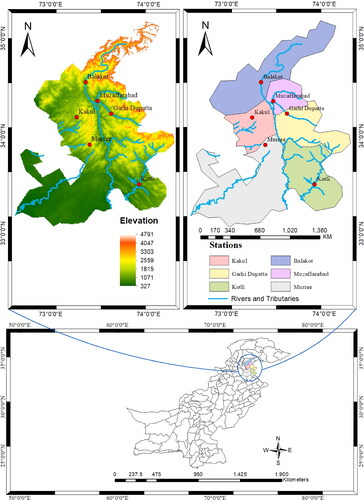
Climatically, the study region varies from mild microthermal (cool winter) to moderate mesodermal (hot summer) (Rahman et al. 2018). Meteorologically, there are two major sources of precipitation in the selected study region; the southeastern monsoons cause rainfall in the summer season, sometimes continuing till the start of autumn (June to September), and the source of rainfall in the winter season (December to February) is western disturbances (Khan et al. 2020). These are major sources of seasonal precipitation in the selected study region. Seasonal variation of precipitation and spatial patterns of drought in the selected study region significantly affects the linked ecosystem, hydroelectric power generation, agricultural yield and industrial production. The present study sought to investigate the spatial patterns of inter-seasonal drought persistence. However, the lack of long-term records from reliable gauged meteorological stations is major dilemma of meteorological and hydro-climatic studies (Ahmed et al. 2018). Monthly total rainfall (mm) and minimum, maximum (average) temperature (°C) data ranging from 1970 to 2016 were obtained from Karachi Data Processing Center (KDPC) through Pakistan Meteorological Department (PMD).

2.2. Standardized precipitation index (SPI)

The Standardized Precipitation Index (SPI) proposed by (Mckee et al. 1993) extensively monitors drought conditions. SPI is recommended by World Meteorological Organization (WMO) for monitoring meteorological drought at various time scales (Hayes et al. 2011). For the calculation of SPI, 32 varying distributions have been used to fit the cumulative monthly precipitation time series data (Stagge et al. 2014; Spiess 2014) and then use the inverse standardized normal distribution to attain the outcome of drought index values. SPI is a dimensionless index where negative values show drought conditions and positive values indicate wet conditions. The findings of Guttman (1998) show that spectral characteristics of SPI are spatially invariant and can be used in any part of the world for assessing drought intensity, magnitude and duration.

2.3. Seasonal drought frequency and inter-seasonal drought persistence

This study uses a 3-month time scale to calculate SPI for inter-seasonal drought persistence and seasonal drought frequency. The distribution of seasons is considered as (1) the winter season comprises ‘December, January and February’; (2) the spring season includes ‘March, April and May’; (3) the summer season comprises ‘June, July and August’, and (4) the autumn season includes ‘September, October and November’. Here meteorological drought is classified according to (Mckee et al. 1993), and continuously negative values of SPI will define a drought period. Whereas the seasonal drought frequency is calculated as the total number of years in which drought occurs $(\mathit{SPI}\le 0)$ in each season at selected meteorological stations. Moreover, the seasonal meteorological drought persistence is defined by (Mckee et al. 1993) as two successive seasons in which SPI contains negative values.

Furthermore, seasonal drought frequency is calculated as the number of years in which drought event occurs, that is SPI have negative values $(\mathit{SPI}\le 0)$ divided by the total number of years of data being used in each climatic zone. This study uses 47 years of precipitation data for calculating SPI at each meteorological station. If drought occurs for 20 years in a particular season, say (spring), then the drought frequency (probability) will be 20/47 or 43%.

Furthermore, inter-seasonal drought persistence describes drought conditions that persist from one season to the subsequent season. The current study assessed drought persistence as winter-spring, spring-summer, summer-autumn and autumn-winter. The presence of drought persistence features at each meteorological station is expressed in terms of the probability of drought persistence. For each climate division, the probability of inter-seasonal drought persistence is calculated as the total number of years exhibiting drought persistence from one season to the subsequent season divided by the total number of years in which drought occurs during the first season in that climate division. For instance, if a climate division exhibits 20 years in which drought occurs in the spring season and drought conditions persist into the summer season for ten years, then the probability of drought persistence will be 10/20 or 50%. Moreover, the current study categorizes SPI into a binary variable: drought occurrence =1 and no drought occurrence = 0.

Similarly, inter-seasonal drought persistence is analysed to describe the influence of subsequent season’s moisture conditions based on the current season’s moisture conditions (Ford and Labosier 2014). As each of the seasons comprises 3-months, so SPI at a 3-month lead time scale is the most appropriate index to predict and analyse inter-seasonal drought persistence. Moreover, the present study employs the Bayesian Logistic Regression Model to examine inter-seasonal drought persistence.

2.4. Bayesian logistic regression model

The Logistic regression model is a special case of a generalized linear model to predict binary responses with one or more binary and continuous explanatory variables. As prediction of drought persistence in the upcoming season (binary variable) based on SPI of the current season (continuous variable) using a linear regression model can lead to several issues like non-normality of errors and the range violation of predicted probabilities from 0 to 1 (Kutner et al. 2005). Moreover, the logistic regression model is more often used to examine binary response variables based on one or more explanatory variables. Various studies have employed logistic regression for the prediction of drought occurrences and drought persistence (Peng et al. 2002; Ford and Labosier 2014; Meng et al. 2017). The method of Maximum Likelihood Estimation (MLE) is used to estimate the parameters of the logistic regression model, which maximizes the relevant likelihood function. However, this frequentist method for quantifying uncertainty involves closed-form issues, and the MLEs obtained from iterative methods are only point estimates of parameters, leading to several inferential issues. Whereas Bayesian Logistic Regression Model (BLRM) is more flexible method to model the relationship between a binary response variable and one or more independent variables. BLRM is robust to outliers and also can handle missing data more effectively. Moreover, BLRM incorporates prior parameter information and leads to more accurate predictions. Therefore, due to certain advantages, the Bayesian Logistic Regression Model (BLRM) is proposed to investigate the persistence of drought from one season to the subsequent season. The BLRM considers the parameters of the model as random variables with some specified prior distributions (Mahanta et al. 2015; Gebrie 2021). Estimating logistic regression model parameters through the Bayesian framework had superior results than MLEs, even for small samples, as it allows the probabilistic interpretation of the estimates (Chang et al. 2018).

Let $X_{(s-1)t}$ be the values of SPI-3 of the previous season and $Y_{(s)t}$ be the binary response variable representing the drought occurrence in the current season defined as $$Y_{(s)t}=\left\{\begin{array}{cc}1& \mathit{drought}\mathit{persistence}\\ 0& no\mathit{drought}\mathit{persistence}\end{array}\right\}$$

The frequentist’s standard logistic sigmoid function defined as (1) $${\eta }_t=P(Y_{(s)t}=1|X_{(s)t})=\frac{e^{{\beta }_0+{\beta }_1{X}_{(s-1)t}}}{1+e^{{\beta }_0+{\beta }_1{X}_{(s-1)t}}}=\frac{1}{1+e^{-({\beta }_0+{\beta }_1{X}_{(s-1)t})}}$$(1) where ${\eta }_t$ is interpreted as the probability of drought occurrence in the current season and can take values 0 to 1. The inverse of the logistic function can be modelled as the link function of the logistic regression model, defined as (2) $$g\left({\eta }_t\right)=\hspace{0.17em}\ln \hspace{0.17em}\left(\raisebox{1ex}{${\eta }_t$}\!\left/ \!\raisebox{-1ex}{$1-{\eta }_t$}\right.\right)={\beta }_0+{\beta }_1{X}_{(s-1)t}$$(2) where $\hspace{0.17em}\ln \hspace{0.17em}\left(\raisebox{1ex}{${\eta }_t$}\!\left/ \!\raisebox{-1ex}{$1-{\eta }_t$}\right.\right)={\beta }_0+{\beta }_1{X}_{(s-1)t}$ represents the log odds ratio of drought occurrences. The parameters of the frequentist logistic regression model are estimated by MLE, which faces certain estimation issues.

Likelihood Function:

Consider a sample of $n$ independent realizations following the Bernoulli distribution with probability ${\eta }_t=P(Y_{(s)t}|X_{(s-1)t}=1)$ as defined in equation (1)(1) $${\eta }_t=P(Y_{(s)t}=1|X_{(s)t})=\frac{e^{{\beta }_0+{\beta }_1{X}_{(s-1)t}}}{1+e^{{\beta }_0+{\beta }_1{X}_{(s-1)t}}}=\frac{1}{1+e^{-({\beta }_0+{\beta }_1{X}_{(s-1)t})}}$$(1) . The likelihood function of the observed dataset can be defined as (Madigan et al. 2005), (3) $$L(y_{(s)t}|{\beta }_j)=\prod _{t=1}^n\left[{\left({\eta }_t\right)}^{y_{(s)t}}{\left(1-{\eta }_t\right)}^{1-y_{(s)t}}\right]=\prod _{t=1}^n\left[{\left(\frac{e^{{\beta }_0+{\beta }_1{X}_{(s-1)t}}}{1+e^{{\beta }_0+{\beta }_1{X}_{(s-1)t}}}\right)}^{y_{(s)t}}{\left(1-\frac{e^{{\beta }_0+{\beta }_1{X}_{(s-1)t}}}{1+e^{{\beta }_0+{\beta }_1{X}_{(s-1)t}}}\right)}^{1-y_{(s)t}}\right]$$(3) where ${\beta }_j=({\beta }_0,{\beta }_1)$ is the set of coefficients, in which ${\beta }_0$ is the intercept term and ${\beta }_1$ is the coefficient (parameter) of the only predictor $X_{(s)t}.$

The prior distribution of parameters:

The selection and specification of appropriate prior distribution in Bayesian Inference play an important role. The Bayesian estimation of parameters required the appropriate specification of the prior distribution for all the unknown parameters of the Logistic Regression Model (LRM). Accurate specification of informative prior distribution can lead to better Bayesian estimates because MLEs in LRM for small samples are biased (Rashwan and Elderney 2016). Usually, the most common prior distribution for the logistic regression model parameters is the Gaussian distribution, i.e. ${\beta }_j\sim N({\mu }_j,{\sigma }_j).$ The informative normal prior distribution of the parameters ${\beta }_j$ can be defined as (4) $$g({\beta }_j)=\frac{1}{\sqrt{2\pi {\sigma }_j^2}}{e}^{-\frac{1}{2}\left\{{\left(\frac{{\beta }_j-{\mu }_j}{{\sigma }_j}\right)}^2\right\}}$$(4)

Student’s t-distribution, Laplace and Cauchy can be used as prior for parameters of the LRM, but normal prior gives more consistent results (Hassan 2020).

Posterior Distribution:

Bayesian estimation defines the parametric uncertainty in terms of prior belief. The posterior distribution of unknown parameters ${\beta }_j=({\beta }_0,{\beta }_1)$ of the LRM with normal priors is proportional to the product of the likelihood function and prior distribution of parameters (Suleiman et al. 2019), (5) $$f({\beta }_j|y_{(s)t})\propto \prod _{t=1}^n\left[{\left(\frac{e^{{\beta }_0+{\beta }_1{X}_{(s-1)t}}}{1+e^{{\beta }_0+{\beta }_1{X}_{(s-1)t}}}\right)}^{y_{(s)t}}{\left(1-\frac{e^{{\beta }_0+{\beta }_1{X}_{(s-1)t}}}{1+e^{{\beta }_0+{\beta }_1{X}_{(s-1)t}}}\right)}^{1-y_{(s)t}}\right]\ast \prod _{j=0}^1\frac{1}{\sqrt{2\pi {\sigma }_j^2}}{e}^{-\frac{1}{2}{\left(\frac{{\beta }_j-{\mu }_j}{{\sigma }_j}\right)}^2}$$(5)

The analytical solution of the posterior distribution stated in equation (5)(5) $$f({\beta }_j|y_{(s)t})\propto \prod _{t=1}^n\left[{\left(\frac{e^{{\beta }_0+{\beta }_1{X}_{(s-1)t}}}{1+e^{{\beta }_0+{\beta }_1{X}_{(s-1)t}}}\right)}^{y_{(s)t}}{\left(1-\frac{e^{{\beta }_0+{\beta }_1{X}_{(s-1)t}}}{1+e^{{\beta }_0+{\beta }_1{X}_{(s-1)t}}}\right)}^{1-y_{(s)t}}\right]\ast \prod _{j=0}^1\frac{1}{\sqrt{2\pi {\sigma }_j^2}}{e}^{-\frac{1}{2}{\left(\frac{{\beta }_j-{\mu }_j}{{\sigma }_j}\right)}^2}$$(5) cannot be evaluated. Instead, the marginal posterior distribution for each parameter of LRM is obtained from joint posterior distributions using Markov Chain Monte Carlo (MCMC) simulations with Gibbs sampling. Gibbs sampling is a computationally convenient algorithm that is a special case of the Metropolis-Hastings algorithm used for Bayesian inference. MCMC simulations are used to obtain random samples from complex and multidimensional probability distributions where direct sampling is impossible. The expected value of the marginal posterior distribution of each parameter of LRM ${\beta }_j$ will be considered as estimated regression coefficients of the BLRM.

3. Results

Six synoptic meteorological stations were selected from the upper catchment area of the Jhelum River in northeastern Pakistan. Descriptive statistics of the average monthly precipitation at selected meteorological stations are given in Table 1. These meteorological records define the climate of the stations. The precipitation of the selected stations is used as an input meteorological variable to calculate SPI. The SPI at 3-month time scale is calculated using 32 varying probability distributions fitted on input meteorological variables. The best-fitted distribution is selected based on the minimum Bayesian Information Criterion (BIC) for standardization. The best-fitted distribution at each station with respective BIC values is given in Table 2. For instance, the Gumbel distribution was found to be more appropriate for Balakot station with a minimum value of BIC (-1777.45). The Gumbel distribution is also selected as the best-fitted distribution for Murree and Muzaffarabad stations with minimum values of BIC as (-1614.46) and (-1540.48), respectively. The Rayleigh distribution has proven its candidacy for Kakul station with minimum BIC (-1170.1). The Logistic distribution is selected for Garhi Dupatta with BIC (-1727.82), whereas the Generalized Extreme Value (GEV) distribution is chosen as an appropriately fitted distribution for Kotli station with a minimum value of BIC (-1478.21). Figure 2 shows the histogram of 3-months of accumulated precipitation data and appropriate fitted theoretical and empirical distribution for all the selected stations. As precipitation data at some stations have extreme values for which thick-tailed distributions have been selected as appropriate distribution. Figure 3 illustrates the goodness of fit by observing the p-p plot of empirical vs. theoretical probabilities at all selected stations. The appropriately fitted distributions are used to calculate the cumulative distribution of the data points, which are then standardized using normal probability distribution to get SPI-3. The temporal behaviour of SPI-3 illustrates the dry and wet conditions shown in Figure 4. Moreover, the annual seasonal rainfall variations across all the selected meteorological stations and their respective climatic features are given in Table 3. According to climate classification, the study area has an almost homogenous climate with quite diverse topographic characteristics. The elevation of stations varies from 614 (Kotli) to 2291 m (Murree). According to Köppen’s (1884) classification, the climate of Murree station is categorized as subtropical highland, whereas all the other stations are classified as humid subtropical. Furthermore, there is substantial seasonal variation in the rainfall at selected meteorological stations.

Figure 2. Histograms of precipitation data and varying fitted distributions for SPI-3.

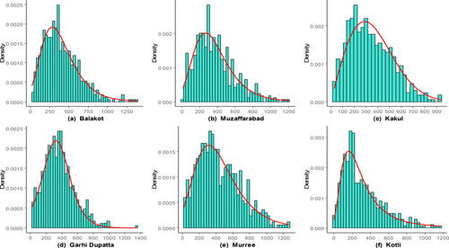
Figure 3. A q-q plot of empirical vs. theoretical distributions for SPI-3 at selected meteorological stations.

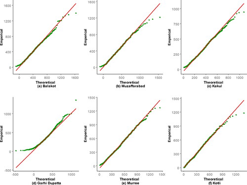
Figure 4. Temporal variations of SPI-3 at selected meteorological stations.

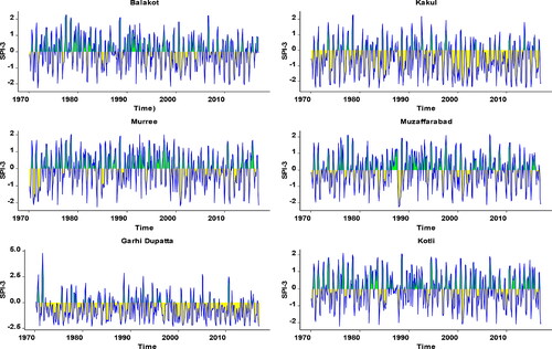
Table 1. Descriptive analysis of precipitation during the period 1971–2017 of selected meteorological stations.

Station	Mean	1st quartile	Median	3rd quartile	Max	Std. dev.
Balakot	132.7	46.9	101.1	187.2	914.9	121.0969
Kakul	111.44	39.38	85.6	161.22	494.6	93.17354
Murree	146.2	47.2	112.2	216.1	704.3	127.193
Muzaffarabad	124.37	43.65	97.2	176.03	721.0	113.1248
Garhi Dupatta	122.14	46.92	97.7	172.2	570.5	100.0412
Kotli	104.15	29.18	69.25	141.15	711.0	109.139

Table 2. Best-fitted probability distributions for the calculation of SPI-3 with their respective BIC values at selected meteorological stations.

Station	Distribution	BIC
Balakot	Gumbel	−1777.45
Kakul	Rayleigh	−1170.10
Murree	Gumbel	−1614.46
Muzaffarabad	Gumbel	−1540.48
Garhi Dupatta	Logistic	−1727.82
Kotli	Generalized Extreme Value	−1478.21

Table 3. Seasonal rainfall variations and climatic features of selected meteorological stations.

Stations	Longitude (N)	Latitude (E)	Elevation (m)	Climate	Seasonal rainfall mm/annum
					Winter	Spring	Summer	Autumn
Balakot	72̊ 21′	34̊ 33′	995	Humid subtropical	308.99	363.17	708.66	211.30
Kakul	73̊ 15′	34̊ 11′	1308	Humid subtropical	228.21	320.10	604.03	184.99
Murree	73̊ 39′	33̊ 91′	2291	Subtropical highland	345.82	363.72	799.49	245.11
Muzaffarabad	73̊ 29′	34̊ 22′	702	Humid subtropical	296.82	333.17	673.58	188.82
Garhi Dupatta	73̊ 37′	34̊ 13′	814	Humid subtropical	324.88	360.30	588.79	191.75
Kotli	73̊ 54′	33̊ 31′	614	Humid subtropical	216.54	240.46	637.16	155.69

At Balakot station, the average annual rainfall for the summer season is 708.66 mm, whereas the average annual rainfall for the autumn season is 211.3 mm. Similar seasonal wet and dry patterns were observed for other meteorological stations.

The study area received the most rainfall during summer, and significantly less rainfall was observed in autumn. These seasonal dry and extreme wet patterns cause extreme climate hazards like severe drought conditions and mass flash flooding events in the region.

3.1. Drought frequency and inter-seasonal drought persistence

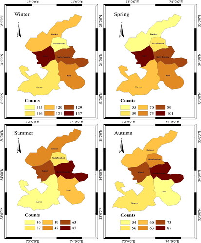
The binary outcome of drought is classified as $\mathit{SPI}\le 0$ is considered as drought and $\mathit{SPI}>0$ specifies as no drought for all seasons at any meteorological station. Figure 5 shows the temporal variability of drought occurrence $\mathit{SPI}\le 0$ as the number of months with drought per annum. Here red lines show the band of maximum and minimum no of months with drought per annum at each station. Figure 6 shows the season-wise count maps of drought occurrences at all selected stations. This visual representation depicts significant spatial and seasonal variation. The highest drought counts have been observed during winter (115–137) across all selected climatic divisions whereas significantly less drought prevails in summer. It has been observed that the Kakul and Garhi Dupatta stations are more vulnerable to drought across all seasons, whereas Muzaffarabad and Murree stations are less prone to drought.

Figure 5. Temporal behaviour of $\mathit{SPI}\le 0$ selected meteorological stations.

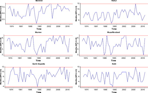
Figure 6. Seasonal drought counts (total number of moths with $\mathit{SPI}\le 0$) at selected stations.

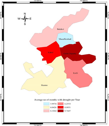
Furthermore, Figure 7 shows the average number of months with drought per year at all selected stations. The average number of drought months varies from 1 to 9 months at Balakot station, with an average of 6 months with drought. While at Kakul station, the number of months with $\mathit{SPI}\le 0$ in each year varies from 5 to 12 months, with an average of 8.0851 months. The average number of months $\mathit{SPI}\le 0$ at all selected meteorological stations varies from 5.9574 to 8.7447 months.

Figure 7. Average number of months with $\mathit{SPI}\le 0$ per year at each selected station.

Moreover, the seasonal drought frequency is calculated as the total number of months with $\mathit{SPI}\le 0$ divided by the total number of months from January 1971 to December 2017. Similarly, seasonal drought frequency for winter, spring, summer and autumn seasons is calculated. Figure 8 shows seasonal drought frequency across all climate divisions as a percentage of years between 1971 and 2017. Drought frequency during all seasons reveals substantial spatial and seasonal variations. The average drought frequency is 89.1, 54.2, 37.3 and 49.3% for winter, spring, summer and autumn seasons, respectively, for the whole study area (Table 4). The average seasonal drought frequency for the winter season is significantly higher than other seasons, whereas, for the summer season, it is the least among all the seasons. Similarly, the average drought frequencies for Kakul and Garhi Dupatta stations are significantly higher, whereas Muzaffarabad and Murree stations experienced less average drought frequency across all seasons. The difference in drought frequency between different regions and seasons indicates spatial and seasonal patterns in drought frequency. Figure 9 shows the inter-seasonal drought persistence at all individual meteorological stations.

Figure 8. Seasonal drought frequency as a percentage of total years (1070–2016) at each station.

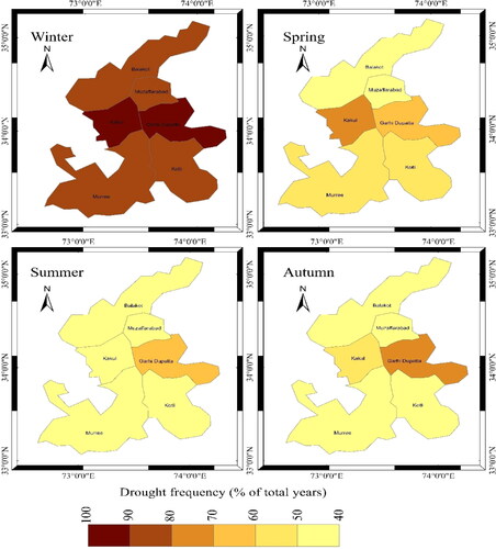
Figure 9. Drought persistence percent probability for all seasons in the selected stations.

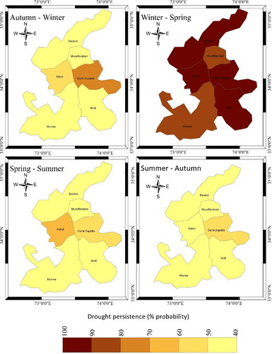
Table 4. Regional average of seasonal drought frequency as measured by percent probability.

Stations	Winter	Spring	Summer	Autumn	Average
Balakot	87.0	39.9	34.1	43.5	51.1
Kakul	99.3	73.2	45.7	52.9	67.8
Murree	84.1	50.7	26.1	40.6	50.4
Muzaffarabad	83.3	42.8	26.8	45.7	49.6
Garhi Dupatta	93.5	64.5	63.0	73.9	73.7
Kotli	87.7	54.3	28.3	39.1	52.4
Average	89.1	54.2	37.3	49.3

These maps show that inter-seasonal drought persistence is strongest in winter to spring, whereas it is less prevalent between summer and autumn. The average inter-seasonal drought persistence in the whole study region is 42.8, 91.7, 48.2 and 21.9% for winter, spring, summer and autumn seasons, respectively (Table 5). At Kakul station, the winter-to-spring drought persistence is 100%, and if drought occurs during the winter season, it will be prolonged till the end of the spring season.

Table 5. Regional average of seasonal drought persistence as measured by percent probability.

Stations	Autumn to winter	Winter to spring	Spring to summer	Summer to autumn	Average
Balakot	40.0	92.7	36.2	5.0	43.5
Kakul	52.6	100.0	68.3	17.8	59.7
Murree	35.3	85.7	44.4	3.6	42.3
Muzaffarabad	41.7	84.7	37.8	1.6	41.5
Garhi Dupatta	72.9	96.6	56.3	52.9	69.7
Kotli	35.5	90.7	46.2	3.7	44.0
Average	46.3	91.7	48.2	14.1

The prolonged meteorological drought can severely affect the moisture conditions. Moreover, the autumn-to-winter and spring-to-summer seasons show similar inter-seasonal drought persistence patterns and did not demonstrate any considerable spatial variability. Furthermore, summer-to-autumn drought persistence is significantly low at all meteorological stations except for Garhi Dupatta. On the other hand, the inter-seasonal drought persistence at Garhi Dupatta station is remarkably high for all seasons. These graphical and numerical results show the substantial temporal and spatial variability in the inter-seasonal drought persistence.

3.2. Bayesian logistic regression results

The results shown in section 3.1 demonstrates that meteorological drought in the study region (northeastern part of Pakistan) can persist seasonally, and inter-seasonal drought persistence exhibits massive spatial and temporal variability. However, Bayesian Logistic Regression Model (BLRM) is used to assess the impact of moisture conditions in one season to subsequent seasons at all selected meteorological stations. The model binary response variable is drought occurrence in the current season (drought = 1, no drought = 0), and the explanatory variable is the SPI of the previous season. The output of the model is the log odds ratio of drought occurrence in the current season, and the estimated parameter $(\beta )$ of the BLRM represents the relationship between response and explanatory variables. However, Bayesian logistic regression analysis cannot reveal the cause-and-effect relationship. For instance, when the $(\beta )$ value is negative, the odds of drought occurrence in the current season are negatively related to the SPI value in the previous season. This reflects that a decrease in the previous season’s SPI would increase the odds of drought occurrence in the subsequent season and vice versa.

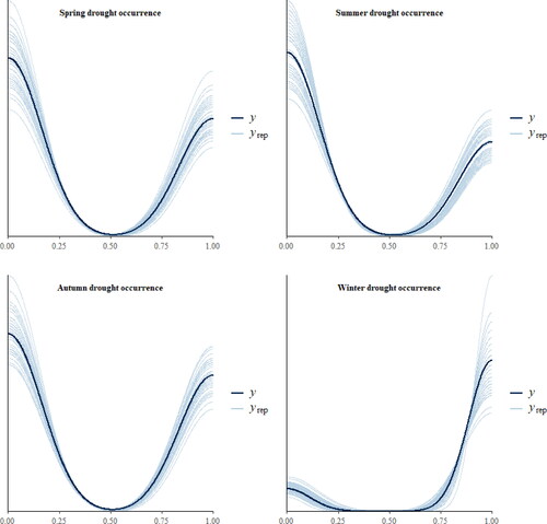
Some graphical model diagnostics are used to assess the Markov Chain Monte Carlo (MCMC) convergence and validate best-fitted BLRM. Generally, trace plots are considered the best graphical method to check the convergence of MCMC simulations. The trace plots given in Figure 10 feature 1000 sequential draws from the posterior distribution of the Bayesian logistic regression coefficient associated with the previous season’s SPI values. These trace plots are reasonably stable as chains in each trace plot centred around one value and well overlapped. The other checkup for MCMC simulation runs is posterior predictive checks. Figure 11 shows posterior predictive checks for inter-seasonal drought persistence analysis for all four seasons at Balakot. These posterior predictive checks compare observed data with simulated data using fitted BLRM, which are used to assess the predictive validity of the fitted model. The dark blue line in each plot of Figure 11 represents the observed data, and the light blue lines demonstrate the simulated data sets through posterior predictive distributions. These plots identify that observed data sets are lying in the centre of simulated datasets, which shows the better predictive performance of the fitted BLRM.

Figure 10. Posterior trace plots of the logistic regression coefficient associated with predictor (SPI) for all seasons at Balakot station.

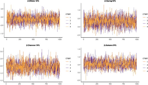
Figure 11. Posterior predictive checks for seasonal drought occurrence at Balakot station.

Similarly, histograms with the posterior distribution are obtained by combining the values of all the chains for the estimated coefficient (β) for inter-seasonal drought persistence analysis. Moreover, Figure 12 presents histograms of posterior samples of β coefficients. These posterior samples can be used to perform inference. The BLRM regression coefficient β value describes the variability in odds ratio of drought occurrence in current season as function of SPI values of prior season. The probability distributions generated by β values more comprehensively describes the relationship between probability of drought occurrence in one season and SPI values of prior season. Figure 13 shows the plot of predicted probabilities of drought occurrence in the current season as a function of SPI values of the previous season for all four inter-seasonal drought persistence analyses at Balakot station. These plots can deduce the inter-seasonal drought persistence strength for all the seasons. Figure 13(a) shows a slightly negative but non-significant relationship between probabilities of drought occurrence in the spring season and SPI values of the winter season. The variability in probability of drought occurrence in spring season is weak function of SPI values of winter season as β coefficient is non-significant.

Figure 12. Histograms with the distribution of posterior values combining all chains by estimated parameters (β) for all seasons at Balakot station.

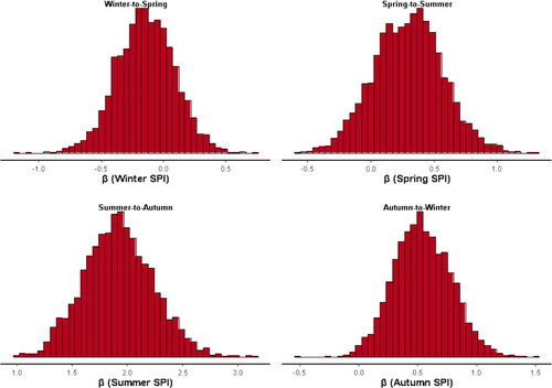
Figure 13. Seasonal drought probability distributions as a function of the previous season’s SPI for Balakot station.

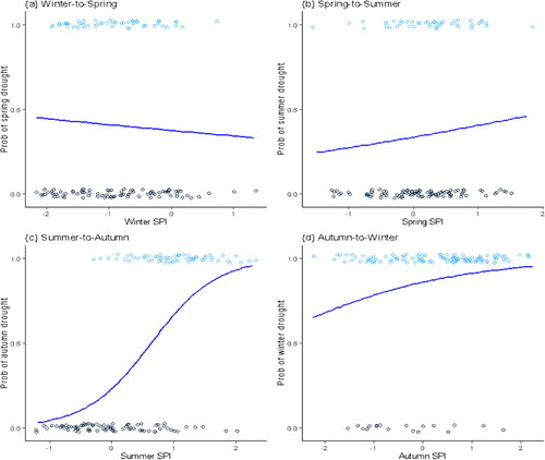
Similarly, Figure 13(b) and (d) shows drought occurrence probability distributions as a function of the previous season’s SPI values for spring-to-summer and autumn-to-winter seasons. Again, the probability of drought in the given season has shown a weak positive relationship with the SPI values of the previous season. Furthermore, β values of BLRM corresponding to these two seasonal combinations are statistically non-significant. Moreover, Figure 13(c) clearly illustrates a significant positive relationship between drought occurrence in the autumn and summer season SPI values at Balakot station. The autumn drought probabilities vary strongly as a function of summer SPI. This relation illustrates that the summer moisture conditions strongly affect the autumn drought occurrence, which has considerable ramifications for seasonal drought prediction.

3.2.1. Drought occurrence odds ratios

The BLRM is employed for various inter-seasonal drought persistence analyses at all selected stations to quantify the change in the response variable (drought occurrence in the current season) corresponding to a change in the explanatory variable (SPI values of the previous season). The estimated coefficients (β) of BLRM are converted to $e^{\beta }$ represent the change in drought occurrence odds ratio as a function of one unit increase in the previous season’s SPI. The inter-seasonal drought persistence odds ratios output from BLRM is presented in various maps of Figure 14. The station with an odds ratio < 1 indicates a decreased odds ratio of drought occurrence in the current season when SPI of the previous season increases, whereas stations with an odds ratio > 1 showing that a positive increase in the odds ratio of drought occurrence in the current season corresponding to increase in previous season’s SPI. The estimated coefficients, odds ratios, Standard Error (SE) of estimates and 99% Credible Intervals (CI) of fitted BLRM for all inter-seasonal drought persistence analyses at all the selected meteorological stations are given in Table 6. The bold values represent statistically significant odds ratios at α < 1%. The relationship between spring drought occurrence and SPI of the winter season (Figure 14(a)) is negative but non-significant for all the stations. For instance, at Balakot station for winter to spring, the odds ratio value is 0.87, which is less than one showing that with a 1 unit increase in SPI of the winter season, the odds of drought occurrence in the spring season will decrease by 13 to 100%. The relationship between summer drought occurrence and SPI of the spring season (Figure 14(b)) is positive for all the stations but significant for only one station (Garhi Dupatta). This significant result shows that a 1 unit increase in SPI of the spring season will cause a 75% increase in the odds of drought occurrence in summer. Moreover, at Balakot station, the odds ratio’s value is significant for the summer-to-autumn season (6.78). It shows that one unit increase in SPI of the summer season will cause 5.78 times to increase in odds of autumn drought occurrence. Moreover, the relationship between SPI and drought occurrence for winter-to-spring seasons for all the stations is negative, while all the other inter-seasonal relationships are positive, of which some odds ratios are significant. Moreover, statistically, significant odds ratios are presented in bold form stations in maps of Figure 14. The non-significant results suggest that seasonal drought prediction at those stations based on a single meteorological indicator, such as SPI values, would be challenging. At the same time, these significant odds ratios illustrate that the previous season’s SPI values significantly influence drought occurrence in subsequent seasons in the selected study region. These results can be helpful for water resource management for industrial and agricultural development in the upcoming seasons.

Figure 14. Odds ratio for various seasons in the selected stations. The bold form stations are significant at 1%.

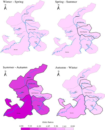
Table 6. Estimated coefficients, odds ratios (OR), standard errors (SE) of estimates, and 99% credible intervals (CI) of odds ratios obtained from Bayesian logistic regression models for inter-seasonal combinations at all the selected stations.

					99% CI (OR)
Stations	Season	Coefficient	OR	SE	Lower	Upper
Balakot	Winter-to-Spring	−0.1	0.87	0.2	0.47	1.56
	Spring-to-summer	0.3	1.35	0.3	0.68	2.76
	Summer-to-autumn	1.9*	6.78	0.3	3.29	15.51
	Autumn-to-winter	0.5	1.7	0.2	0.98	3.20
Kakul	Winter-to-spring	0	1.00	0.3	0.48	2.11
	Spring-to-summer	0.3	1.33	0.3	0.69	2.56
	Summer-to-autumn	1.9*	6.94	0.3	3.23	18.48
	Autumn-to-winter	0.2	1.16	0.4	0.42	3.28
Murree	Winter-to-spring	0.0	0.97	0.2	0.56	1.65
	Spring-to-summer	0.3	1.41	0.3	0.75	2.93
	Summer-to-autumn	2.2*	8.61	0.4	3.61	23.37
	Autumn-to-winter	0.8*	2.24	0.2	1.24	4.32
Muzaffarabad	Winter-to-spring	−0.1	0.88	0.2	0.52	1.54
	Spring-to-summer	0.2	1.23	0.3	0.63	2.50
	Summer-to-autumn	1.9*	7.01	0.3	3.39	16.84
	Autumn-to-winter	0.7	1.93	0.2	1.09	3.56
Garhi Dupatta	Winter-to-spring	−0.2	0.8	0.2	0.44	1.43
	Spring-to-summer	0.6*	1.75	0.2	1.04	3.19
	Summer-to-autumn	0.8*	2.17	0.2	1.23	4.29
	Autumn-to-winter	0.0	1.00	0.3	0.52	2.15
Kotli	Winter-to-spring	−0.2	0.82	0.2	0.44	1.51
	Spring-to-summer	0.4	1.47	0.3	0.73	2.87
	Summer-to-autumn	1.9*	6.46	0.3	2.90	16.21
	Autumn-to-winter	0.6*	1.87	0.2	1.02	3.76

3.3. Limitations and suggestions for future work

Current study has used BLRM to identify the spatial patterns of seasonal drought frequency and inter-seasonal drought persistence. The drought persistence in the given season was predicted using SPI values of previous season. The major limitation of the study is that it is restricted to predict drought persistence of the subsequent season only which can be extended for several forthcoming seasons. For future studies the spatiotemporal patterns of inter-seasonal drought persistence can be studied by using other machine learning algorithms such as Naïve Bayes classifier, Random Forest and Bayesian Network theory.

Moreover, current study only emphasizes on meteorological drought; however, researchers can include other hydrological and agricultural parameters to assess, monitor and forecast hydrological and agricultural drought. Remote sensing and soil moisture variables can be added to the model for better prediction of drought persistence. Moreover, current study have used SPI for drought characterization, future studies can be extended by using other SDIs which is subject to availability of data related to meteorological variables.

4. Discussion

The selected study region has structural importance for other country regions situated downstream. As much of the agricultural land of the country is irrigated through IBIS. Therefore, drought occurrence and inter-seasonal drought persistence in the study region directly affect the country’s agricultural production. The main goal of the study was to quantify seasonal drought occurrence and prediction of inter-seasonal drought persistence across the study region. Monthly precipitation data have been used to calculate SPI with a 3-month time scale, which is further used to calculate seasonal drought frequency and inter-seasonal drought persistence at all selected meteorological stations. SPI-3 is sufficient to reflect all climate divisions’ short- and medium-term moisture conditions. The descriptive analysis reveals that the study region receives most of its precipitation from monsoons during summer and western disturbances during winter. Sometimes monsoon season starts in summer and continues till the mid-autumn season. However, most of the time, autumn and spring seasons cannot receive sufficient rainfall to maintain moisture levels. In that situation, the vegetation and agricultural production in the region are highly dependent on the previous season’s moisture conditions. The drought frequency during winter is significantly high, whereas summer is the least dry season across the study region.

Furthermore, the drought frequency substantially varies from one station to another. For example, Kakul and Garhi Dupatta stations encountered more drought episodes across all seasons. The seasonal and spatial drought frequency analysis shows that drought has certain spatial and seasonal patterns in the whole study region (Figures 6–8). Furthermore, we have calculated the probability of drought persistence for each season at all meteorological stations to analyse the relationship between inter-seasonal moisture conditions. Results revealed that inter-seasonal drought persistence strength varies strongly across the study region. Dominant factors for inter-seasonal drought persistence may have temporal relevance. A detailed examination of physical mechanisms on the spatial and seasonal patterns is shown in Figure 9.

The autumn-to-winter inter-seasonal drought persistence has shown much stronger agreement at Garhi Dupatta and Kakul. The possible reason for this autumn-to-winter drought persistence at two stations is the impact of autumn soil moisture deficit. The winter season’s rainfall in the study region is associated with western disturbances, an extratropical storm originating in the Mediterranean region. It is a non-monsoonal precipitation pattern driven by the westerlies. Rich soil moisture conditions in the winter play a vital role in the vegetation of rabi crops. Wheat is one of the rabi season’s most important and signature crops, considered the food security of Pakistan and other regional countries. A soil moisture deficit in the winter season severely affects the rabi crop yield. Early termination of the monsoon season is one of the possible reasons for drought occurrence in the autumn season. The higher drought probabilities in the winter are associated with the region’s late onset of the western disturbance system. Therefore, autumn soil moisture deficit could force strong autumn to winter inter-seasonal drought persistence.

The winter season in the selected study area is mostly considered the dry season. The average drought probability in winter across the whole study region is 89.1%, which is sufficiently large compared to other seasons (Table 4). The winter-to-spring inter-seasonal drought persistence is largely associated with weak western disturbances, thermal conditions of the region, and La Nina events with severe intensity (Khan 2004). The La Nina phenomenon is referred to as cooler than normal ocean surface temperature in the eastern and central Pacific oceans. The anomalies and atmospheric circulation also result in inter-seasonal drought persistence from winter to spring. The average seasonal drought persistence from winter to spring season is significantly high, i.e. 91.7%. The higher probabilities of drought occurrence in the spring are associated with the late onset of the Asian monsoon rainfall system. These possible reasons result in strong winter-to-spring inter-season drought persistence. Whereas summer drought is less prevailing as compared to other seasons. The spring deficit of soil moisture conditions is significantly less prolonged until the summer. Therefore, Kakul and Garhi Dupatta stations have some inter-seasonal drought persistence.

Furthermore, Bayesian logistic regression is used to study the complex relationship between SPI values of a given season and binary response variable (drought occurrence in subsequent seasons). The Bayesian estimation procedure is more flexible than maximum likelihood estimation as it expresses the data as a likelihood function, providing appropriate informative prior distribution and updating the posterior distribution of the parameters of the model-given data. These posterior distributions are further used for inference about the parameters. The study’s outcome suggests that BLRM adequately describes patterns of meteorological drought occurrence. The probabilities associated with BLRM output are generally more interpretable than the logistic regression output. The BLRM output shows a non-significant negative relationship between spring drought occurrence and SPI values in the winter season.

Moreover, this negative relationship has no spatial relevance and prevails across the study region. This weak negative relationship between spring drought occurrence and winter SPI suggests that winter droughts are more likely to continue into spring. At the same time, all the other inter-seasonal drought relationships are positive. These positive relationships suggest that SPI values of the current season positively affect the drought occurrence in subsequent seasons. This is obvious that the autumn season receives fewer precipitations than other seasons due to the weaker Asian monsoon. The two primary factors, including Pacific and Indian Ocean surface temperature and the snow cover in Eurasia and the Himalayan Mountains, are the influencing forces for weakening the South Asian monsoon rainfall system in the autumn season (Yihui and Chan 2005). These external influencing factors usually have long memory that can persist from one season to another. The significant odds ratios related to summer-to-autumn drought persistence suggest that autumn-season drought occurrence has a very strong relationship with SPI values of the summer season. Therefore, the autumn drought occurrence can be predicted using SPI values of the summer season, which can be helpful for water resource managers and farmers for vegetation in the autumn season. None of the authors have analysed the seasonal drought frequency and inter-seasonal drought persistence in northeastern Pakistan (upper catchment area of Jhelum River). Therefore, it is a novel approach to analyse spatial patterns of seasonal drought occurrence and predict inter-seasonal drought persistence using BLRM. The associated outcome of the current study can provide massive guidelines for policymakers to develop effective early warning systems and enhance drought mitigation policies. Reliable prediction of inter-seasonal drought persistence can provide the basis for efficient water resource management and drought-resilient crop management.

5. Conclusion

Drought is one of the most disastrous natural hazards, least understood to monitor, and occurs in virtually all climate divisions around the globe. Understanding the characteristics of widespread drought occurrence is critical for drought monitoring and assessment. Long-term drought impacted agriculture, water supply, linked ecosystem and socio-economic activities. Developing new frameworks and methodologies have significantly enhanced drought monitoring and impact assessment accuracy. The upper catchment area of the Jhelum River in the northeastern part of Pakistan is selected as the study region. The investigation of drought in the selected study region has various perspectives. The primary objective was to study the seasonal drought frequency and inter-seasonal drought persistence. Seasonal drought frequency information is vital in water resource management, crop yield, agriculture development and energy consumption. The study’s secondary objective was to identify the spatial patterns of seasonal drought frequency and inter-seasonal drought persistence by employing Bayesian logistic regression to investigate the probability and odds of drought persistence from one season to the subsequent season. The monthly precipitation data calculate SPI with a 3-month lead time scale. Results presented in Sections 3.1 and 3.2 reveal that inter-seasonal drought persistence has substantial variability across the study region. For instance, the relationship between winter to spring moisture conditions at most of the meteorological stations of the study region is strong, whereas Kakul and Garhi Dupatta stations show moderate inter-seasonal drought persistence for autumn to winter and spring to summer seasons.

Furthermore, based on meteorological indices, Bayesian logistic regression predicts inter-seasonal drought persistence. BLRM outcome indicates that some areas are more prone to drought and vulnerable to inter-seasonal drought persistence. Our results also recommend that Bayesian logistic regression provides a suitable methodology to describe patterns of inter-seasonal drought persistence. The outcome of the study can be helpful for developing drought mitigation policies to cope with the consequences of inter-seasonal drought persistence on aquatic ecosystems and agricultural yield. The analysis and outcome of the study are applicable to the current situation and study region and cannot be generalized to other climatic zones. This is due to multiple factors involved in drought occurrence and its persistence from one season to another, such as precipitation, temperature, solar reflux and evapotranspiration. Moreover, climatic conditions of the regions may vary, and results can be affected by the assessment of drought occurrence. However, the approach and methodology used in the study can be generalized to another climate regime.

Our evaluation of drought frequency analysis and inter-seasonal drought persistence opened several study gates for future inquiry. First, possible modifications to the Bayesian logistic regression model can be made by including more explanatory and axillary variables. Long-term drought persistence can be explored by studying the relationship between drought occurrence in the current season and SPI values of several prior seasons using the higher-order Markov Chain model.

Consent to participate

All authors voluntarily agreed to participate in this research study.

Availability of data and codes

The data and codes used for the preparation of the manuscript are available with the corresponding author and can be provided upon request.

Ethical statement

All procedures followed were in accordance with the ethical standards of the Helsinki Declaration of 1975, as revised in 2000.

Acknowledgments

Their authors extend their appreciation to the Deanship of Scientific Research at King Khalid University for funding this work through Large Groups project under grant number (RGP.2/23/44). This study is supported via funding from Prince Sattam bin Abdulaziz University project number (PSAU/2023/R/1444).

Disclosure statement of interests

The authors declare that they have no known competing financial interests or personal relationships that could have influenced the work reported in this paper.

References

- Adnan S, Ullah K. 2020. Development of drought hazard index for vulnerability assessment in Pakistan. Nat Hazards. 103(3):2989–3010.
- AghaKouchak A, Farahmand A, Melton FS, Teixeira J, Anderson MC, Wardlow BD, Hain CR. 2015. Remote sensing of drought: progress, challenges and opportunities. Rev Geophys. 53(2):452–480.
- AghaKouchak A, Mirchi A, Madani K, Di Baldassarre G, Nazemi A, Alborzi A, … Wanders N. 2021. Anthropogenic drought: definition, challenges, and opportunities. Rev Geophys. 59(2):e2019RG000683.
- Ahmed K, Shahid S, Ismail T, Nawaz N, Wang XJ. 2018. Absolute homogeneity assessment of precipitation time series in an arid region of Pakistan. Atmósfera. 31(3):301–316.
- Bandyopadhyay N, Bhuiyan C, Saha AK. 2020. Drought mitigation: critical analysis and proposal for a new drought policy with special reference to Gujarat (India). Progr Disaster Sci. 5:100049.
- Basharat M. 2019. Water management in the Indus Basin in Pakistan: challenges and opportunities. In: Indus River Basin: Water Security and Sustainability. Elsevier Amsterdam, The Netherlands. p. 375–388.
- Benevolenza MA, DeRigne L. 2019. The impact of climate change and natural disasters on vulnerable populations: a systematic review of literature. Journal of Human Behavior in the Social Environment. 29(2):266–281.
- Byun HR, Wilhite DA. 1999. Objective quantification of drought severity and duration. J Clim. 12(9):2747–2756.
- Chang M, Dalpatadu RJ, Phanord D, Singh AK. 2018. Breast cancer prediction using Bayesian logistic regression. Biostat Bioinform. 2(3):1–5.
- Chiew FHS, Young WJ, Cai W, Teng J. 2011. Current drought and future hydroclimate projections in southeast Australia and implications for water resources management. Stoch Environ Res Risk Assess. 25(4):601–612.
- Dikshit A, Pradhan B, Santosh M. 2022. Artificial neural networks in drought prediction in the 21st century – a scientometric analysis. Appl Soft Comput. 114:108080.
- Edwards DC, McKee TB. 1997. Characteristics of 20th century drought in the United States at multiple time scales. Climo Report 97-2, Dept. of Atmos. Sci., CSU, Fort Collins, CO, 155.
- Fang W, Huang S, Huang G, Huang Q, Wang H, Wang L, Zhang Y, Li P, Ma L. 2019. Copulas‐based risk analysis for inter‐seasonal combinations of wet and dry conditions under a changing climate. Int J Climatol. 39(4):2005–2021.
- Ford T, Labosier CF. 2014. Spatial patterns of drought persistence in the Southeastern United States. Int J Climatol. 34(7):2229–2240.
- Gebrie YF. 2021. Bayesian regression model with application to a study of food insecurity in household level: a cross sectional study. BMC Public Health. 21(1):1–10.
- Ghosh J, Li Y, Mitra R. 2018. On the use of Cauchy prior distributions for Bayesian logistic regression. Bayesian Anal. 13(2):359–383.
- Griffiths WE, Hill RC, Pope PJ. 1987. Small sample properties of probit model estimators. J Am Stat Assoc. 82(399):929–937.
- Guttman NB. 1998. Comparing the palmer drought index and the standardized precipitation index 1. J Am Water Resour Assoc. 34(1):113–121.
- Hassan MM. 2020. A fully Bayesian logistic regression model for classification of ZADA diabetes dataset. SJUOZ. 8(3):105–111.
- Hayes M, Svoboda M, Wall N, Widhalm M. 2011. The Lincoln declaration on drought indices: universal meteorological drought index recommended. Bull Am Meteorol Soc. 92(4):485–488.
- He B, Wu J, Lü A, Cui X, Zhou L, Liu M, Zhao L. 2013. Quantitative assessment and spatial characteristic analysis of agricultural drought risk in China. Nat Hazards. 66(2):155–166.
- Ionita M, Scholz P, Chelcea S. 2015. Spatio‐temporal variability of dryness/wetness in the Danube River Basin. Hydrol Process. 29(20):4483–4497.
- Katipoğlu OM. 2022a. Spatial analysis of seasonal precipitation using various interpolation methods in the Euphrates basin, Turkey. Acta Geophys. 70(2):859–878.
- Katipoğlu OM. 2022b. Prediction of future hydrological droughts with tree-based algorithms. Int Res Eng Sci. 51:51–70
- Katipoğlu OM. 2023. Prediction of streamflow drought index for short-term hydrological drought in the semi-arid Yesilirmak Basin using Wavelet transform and artificial intelligence techniques. Sustainability. 15(2):1109.
- Katipoğlu OM, Acar R. 2022. Space-time variations of hydrological drought severities and trends in the semi-arid Euphrates Basin, Turkey. Stoch Environ Res Risk Assess. 36(12):4017–4040.
- Katipoğlu OM, Acar R, Şenocak S. 2021. Spatio-temporal analysis of meteorological and hydrological droughts in the Euphrates Basin, Turkey. Water Supply. 21(4):1657–1673.
- Khan AH. 2004. The influence of La-Nina phenomena on Pakistan’s precipitation. Pak J Meteorol. 1(1):23–31.
- Khan AN, Atta-Ur-Rahman. 2011. Analysis of flood causes and associated socio-economic damages in the Hindukush region. Nat Hazards. 59(3):1239–1260.,
- Khan N, Sachindra DA, Shahid S, Ahmed K, Shiru MS, Nawaz N. 2020. Prediction of droughts over Pakistan using machine learning algorithms. Adv Water Resour. 139:Article ID:103562.
- Khan N, Shahid S, Ahmed K, Ismail T, Nawaz N, Son M. 2018. Performance assessment of general circulation model in simulating daily precipitation and temperature using multiple gridded datasets. Water. 10(12):1793.
- Köppen W. 1884. Die Wärmezonen der Erde, nach der Dauer der heissen, gemässigten und kalten Zeit und nach der Wirkung der Wärme auf die organische Welt betrachtet. Meteorol Z. 1(21):5–226.
- Kutner MH, Nachtsheim CJ, Neter J, Li W. 2005. Applied linear statistical models.New York: McGraw-Hill Irwin.
- Kuwayama Y, Thompson A, Bernknopf R, Zaitchik B, Vail P. 2019. Estimating the impact of drought on agriculture using the US Drought Monitor. Am J Agric Econ. 101(1):193–210.
- LeSage JP. 1999. Applied econometrics using MATLAB. Toledo, OH: Dept. of Economics, University of Toronto; p. 154–159.
- Li D, Liu B, Ye C. 2022. Meteorological and hydrological drought risks under changing environment on the Wanquan River Basin, Southern China. Nat Hazards. 114(3):2941–2967.
- Li L, Yao W. 2018. Fully Bayesian logistic regression with hyper-LASSO priors for high-dimensional feature selection. J Stat Comput Simul. 88(14):2827–2851.
- Lorenzo-Lacruz J, Vicente-Serrano SM, López-Moreno JI, Beguería S, García-Ruiz JM, Cuadrat JM. 2010. The impact of droughts and water management on various hydrological systems in the headwaters of the Tagus River (central Spain). J Hydrol. 386(1-4):13–26.
- Luo S, Calderón-Urrea A, Yu J, Liao W, Xie J, Lv J, Feng Z, Tang Z. 2020. Chronic and intense droughts differentially influence grassland carbon-nutrient dynamics along a natural aridity gradient. Plant Soil. 449(1-2):1–10.
- Madigan D, Genkin A, Lewis DD, Fradkin D. 2005. Bayesian multinomial logistic regression for author identification. In: AIP Conference proceedings. Vol. 803, No. 1. Melville, NY: American Institute of Physics; p. 509–516.
- Mahanta J, Biswas SC, Roy MK, Islam MA. 2015. A comparison of Bayesian and classical approach for estimating Markov based logistic model. Am J Math Stat. 5(4):178–183.
- McKee TB, Doesken NJ, Kleist J. 1993. The relationship of drought frequency and duration to time scales. In: Proceedings of the 8th Conference on Applied Climatology; Jan 17–22; p. 179–183.
- Meng L, Ford T, Guo Y. 2017. Logistic regression analysis of drought persistence in East China. Int J Climatol. 37(3):1444–1455.
- Mishra AK, Singh VP. 2010. A review of drought concepts. J Hydrol. 391(1-2):202–216.
- Naumann G, Alfieri L, Wyser K, Mentaschi L, Betts RA, Carrao H, Spinoni J, Vogt J, Feyen L. 2018. Global changes in drought conditions under different levels of warming. Geophys Res Lett. 45(7):3285–3296.
- Niaz R, Raza MA, Almazah MM, Hussain I, Al-Rezami AY, Al-Shamiri MMA. 2022. Proportional odds model for identifying spatial inter-seasonal propagation of meteorological drought. Geomatics Nat Hazards Risk. 13(1):1614–1639.
- Noorisameleh Z, Gough WA, Mirza M. 2021. Persistence and spatial–temporal variability of drought severity in Iran. Environ Sci Pollut Res Int. 28(35):48808–48822 (Research Paper No. 45, United States Weather Bureau, Washington, D.C., USA).
- Palmer WC. 1965. Meteorological drought. Vol. 30. US Department of Commerce, Weather Bureau.
- Palmer WC. 1968. Keeping track of crop moisture conditions, nationwide: the new crop moisture index.
- Rahman G, Dawood M, Atta-Ur-Rahman, Samiullah. 2018. Spatial and temporal variation of rainfall and drought in Khyber Pakhtunkhwa Province of Pakistan during 1971–2015. Arab J Geosci. 11(3):1–13.
- Rahman G, Rahman AU, Ullah S, Dawood M, Moazzam MFU, Lee BG. 2021. Spatio-temporal characteristics of meteorological drought in Khyber Pakhtunkhwa, Pakistan. PLoS ONE. 16(4):e0249718.
- Rashwan NI, Eldereny M. 2012. The comparison between results of application Bayesian and maximum likelihood approaches on logistic regression model for prostate cancer data. Appl Math Sci. 6(23):1143–1158.
- Santos JF, Pulido‐Calvo I, Portela MM. 2010. Spatial and temporal variability of droughts in Portugal. Water Resour Res. 46(3):Article ID: W03503.
- Shafer BA, Dezman LE. 1982. Development of surface water supply index (SWSI) to assess the severity of drought condition in snowpack runoff areas. In: Proceeding of the Western Snow Conference.
- Shah D, Mishra V. 2020. Integrated Drought Index (IDI) for drought monitoring and assessment in India. Water Resour Res. 56(2):e2019WR026284.
- Sheffield J, Wood EF. 2008. Projected changes in drought occurrence under future global warming from multi-model, multi-scenario, IPCC AR4 simulations. Clim Dyn. 31(1):79–105.
- Sheffield J, Wood EF, Roderick ML. 2012. Little change in global drought over the past 60 years. Nature. 491(7424):435–438.
- Shiru MS, Shahid S, Alias N, Chung ES. 2018. Trend analysis of droughts during crop growing seasons of Nigeria. Sustainability. 10(3):871.
- Slette IJ, Post AK, Awad M, Even T, Punzalan A, Williams S, Smith MD, Knapp AK. 2019. How ecologists define drought, and why we should do better. Glob Chang Biol. 25(10):3193–3200.
- Sönmez FK, Kömüscü AÜ, Erkan A, Turgu E. 2005. An analysis of spatial and temporal dimension of drought vulnerability in Turkey using the standardized precipitation index. Nat Hazards. 35(2):243–264.
- Soule PT. 1990. Spatial patterns of multiple drought types in the contiguous United States: a seasonal comparison. Clim Res. 1:13–21.
- Spiess AN. 2014. Propagate: propagation of uncertainty. R package version, 1–0. https://CRAN.R-project.org/package=propagate.
- Spinoni J, Naumann G, Carrao H, Barbosa P, Vogt J. 2014. World drought frequency, duration, and severity for 1951–2010. Int J Climatol. 34(8):2792–2804.
- Stagge JH, Tallaksen LM, Xu CY, Van Lanen HA. 2014. Standardized precipitation-evapotranspiration index (SPEI): sensitivity to potential evapotranspiration model and parameters. Hydrol Chang World. 363:367–373.
- Suleiman M, Demirhan H, Boyd L, Girosi F, Aksakalli V. 2019. Bayesian logistic regression approaches to predict incorrect DRG assignment. Health Care Manag Sci. 22(2):364–375.
- Tsakiris G, Pangalou D, Vangelis H. 2007. Regional drought assessment based on the Reconnaissance Drought Index (RDI). Water Resour Manage. 21(5):821–833.
- Ullah W, Wang G, Ali G, Tawia Hagan DF, Bhatti AS, Lou D. 2019. Comparing multiple precipitation products against in-situ observations over different climate regions of Pakistan. Remote Sensing. 11(6):628.
- Vicene-Serrano SM, Beguería S, López-Moreno JI. 2010. A multiscalar drought index sensitive to global warming: the standardized precipitation evapotranspiration index. J Clim. 23(7):1696–1718.
- Wang A, Lettenmaier DP, Sheffield J. 2011. Soil moisture drought in China, 1950–2006. J Clim. 24(13):3257–3271.
- Wang W, Zhu Y, Xu R, Liu J. 2015. Drought severity change in China during 1961–2012 indicated by SPI and SPEI. Nat Hazards. 75(3):2437–2451.
- Wei J, Wang Z, Han L, Shang J, Zhao B. 2022. Analysis of spatio-temporal evolution characteristics of drought and its driving factors in yangtze river basin based on SPEI. Atmosphere. 13(12):1986.
- Wilhite DA,Glantz MH. 1985. Understanding: the drought phenomenon: the role of definitions. Waterinternational. 10(3):111–120.
- Yihui D, Chan JC. 2005. The East Asian summer monsoon: an overview. Meteorol Atmos Phys. 89(1-4):117–142.