Need for pan-India compatibility of geospatial databases in terms of map projections and parameters

Abstract

The present study is taken up to record variations in the extent of area of two polygons—(i) a ground measured area of a university campus, (ii) enclosing the Ganga basin—and to examine the changes in both shape and area of another (iii) polygon covering India under different map projections with various parameters. The exercise brought forth interesting results. Depending on final ranks worked out based on minimum differences in extent of areas and shape distortion in the case of India, it is suggested to adopt either (i) Lambert Conformal Conical (LCC) projection with Everest India-Nepal datum, First Standard Parallel (FSP) 24.50, Second Standard Parallel (SSP) 28.50, Latitude of Origin (LO) 16.253259, Central Meridian (CM) 80.8749 or (ii) LCC projection with WGS 84 datum, FSP 24.50, SSP 28.50, LO 16.253259, CM 80.8749 or (iii) Polyconic with Everest India-Nepal datum, CM 84.50, LO 13.00, for mapping both smaller areas on larger scales and larger areas on smaller scales.

Keywords:

• Map projection
• datum
• parameters
• pan-India

1. Introduction

With the advent of Remote Sensing and Geographical Information Systems (GIS) in the early 1970s, there is an explosion of geospatial data and information. By the end of twentieth century with remote sensing satellites of several countries in space, the availability and use of remote sensing data has increased manifold. Though remote sensing data is basically meant for resource surveys and environmental monitoring and mapping, it is extensively being used for various multifarious purposes. With growth and innovations in technology, various other data gathering and information processing methods came into being and consequently, geospatial information grew leaps and bounds in recent times. Nowadays, computer-based GIS databases have almost replaced earlier computer-based data management systems. The GIS databases are different from computerized databases in that the GIS displays and presents spatial units, features, phenomena as maps as well as the qualitative and quantitative data and information connected with the same maps and/or units. In GIS one can visually appreciate and digitally interact with the spatial circumstances while taking decisions. Geographical Information Systems (GISs) have helped and are helping in not only efficiently storing the invaluable old maps and other archival data and information but also in updating the old maps and processing the data into useful information (Krejčí 2008). The real power and purpose of GISs are in their ability to work as decision support systems.

Everything under the sky comes within the ambit of geography and in every walk of life, be it, individually or collectively and personally or professionally, geospatial information matters to those who care. Maps are invaluable and indispensable tools to study and understand the earth along with its complex network of features and phenomena. With maps and geospatial information going digital, what matters to most of us, is taking the right decisions at the right time quickly to get the best and maximum of benefit out of geospatial circumstances/information and that is where GISs come into picture. Ultimately all this boils down to the so-called Information Technology and its efficient use to draw benefits. In the evolution of human civilization, like copper-age, bronze-age, iron-age, etc., the current stage can be called as information-age. One who has information in his/her hand readily and one who can take quick, good and appropriate decisions ‘under the various geospatial circumstances’ is and will be the winner. That is why geospatial information has become global with local, regional and global implications and requirements. This is the crux of the point in the present experiment—there must be global compatibility among data sets coming in from different sources.

Maps which show locations of features and phenomena, and their spatial distributions and patterns are an essential source and component of GIS databases (Pearson 1990). While making maps manually or digitally what is required is geo-referencing the map or remote sensing data, a process by which remote sensing data and other archival maps are brought into the spherical earth’s framework of longitudes and latitudes and then transformed or projected onto two-dimensional plane or surface to ultimately make maps and information. The transformation/projection of the three-dimensional spherical earth or parts of it onto a two-dimensional surface/paper is what is called map projection (Lapaine et al. 2017).

Surveying to take measurements of locations, distances and heights to make maps involves two reference planes or surfaces—geoidal datum and spheroidal datum to mark elevations and to locate the objects/features respectively on near-spherical earth. A detailed discussion on geoidal and spheroidal datums is outside the purview of this study. A datum is a model surface of the earth that is used as an ‘origin surface’ for mapping. The datum defines the shape and size of the earth ellipsoid (because earth which is compressed at the poles is not a perfect sphere) through a so-called origin/reference surface. A datum is chosen and constructed so as to fit to the true shape of the Earth vis-à-vis the land area of a specific country (Mailing 1992). The best fit between the geoidal datum and spheroidal datum and the mean sea level of any country is finally decided as the origin/reference surface for mapping any part/country of the world. A reference surface and mean sea level of one country need not match with the reference surface/mean sea level of other countries. That is exactly the reason why there are many a local datum/reference surfaces like Australian Datum (GDA 94), European Datum (ETRS 89), North American Datum (NAD 83), Japanese Datum (JGD 2011), Everest 1830 etc. and world level reference surfaces/datums like WGS 84, WGS 72, WGS 64 etc. (Lapaine et al. 2017). With any single country, say India, changing the datum while generating spherical coordinates as well as while assigning map projection, will give different results in respect of areas, distances, directions and shapes. So, each and every country works out the best-fit reference surface/datum and best-fit projection to make their maps in order to have the best possible measures of length, width, height and directions.

Survey of India (SOI) went with Polyconic projection with Everest 1830 and Everest 1830 Modified datum for all its large- and small-scale maps (Ghosh and Dubey 2009). With the implementation of India’s New Map Policy 2005, Survey of India has started producing Open Series Maps (OSMs) with Universal Transverse Mercator (UTM) projection system and WGS-1984 datum (National Map Policy 2005; Ghosh and Dubey 2009). National Spatial Framework (NSF) released by National Remote Sensing Centre of Indian Space Research Organization (NRSC-ISRO) has suggested two projections for maps of India—(i) Polyconic projection with Everest Spheroid with 84° 30′ as Central Median (CM) and 13° 00′ as Latitude of Origin (LO) and (ii) Lambert Conformal Conical (LCC) projection with Modified Everest datum with 13° 45′ 00″ as First Standard Parallel (FSP), 18° 45′ 00″ as the Second Standard Parallel (SSP), 80° 52′ 30″ as Central Meridian and 16° 15′ 19.557972″ as Latitude of Origin. National Spatial Framework (NSF) also suggested Lambert Conformal Conic (LCC) projection with World Geodetic System-84 (WGS 84) datum for 1:50,000 and larger scale maps with local standard parallels, central meridians and latitudes of origin depending upon the latitudinal and longitudinal extent, for different states and regions of India (Misra et al. 2022).

In the process of projection, the spherical three-dimensional model along with its x, y and z coordinates is converted into a flat earth model. That means, a curved surface of the spherical earth is transformed into a flat surface. As it is, in this process, the length and breadth are the first casualties—they get decreased from the original/real world measurements. That means, there cannot be a true one to one representation—a map cannot be a true representation of the real world. A map is only an abstraction of the real world at a reduced scale (Kennedy and Kopp 2000) with some inherent errors.

Depending upon the location of the area/country on the globe, the final maps of the respective area/country if finally produced on different projections with different parameters will have scale, shape, area and directional distortions when compared with each other. Some projections retain true directions, some produce near-true scale, some portray true shape, some give near-true areas. No single map projection truly facilitates to get true directions, distances, areas and shapes of any country or any part of the globe. That is why there are specific projections for specific areas and also specific projections for specific purposes—for example, navigation requires maps with true directions. The general-purpose maps on large scales (1:50,000 and larger) go with projections that give near-true distances and areas.

2. Objectives

The present study is aimed at coming up with suggestion on the best fit projections and parameters in Indian context after examining the differences in the extent of the area and shape of a polygon. A total of three cases are taken up in this study. The first two cases: (i) a University campus area measured on the ground and (ii) the Ganga river basin, to note the area differences and the third is a polygon covering India including its islands to record area and shape differences, under various projections and parameters. Yes, it is known and obvious, when the datum and projections change, the extent of area is likely to change. But how much, is the first question. The second question is whether the projections and related parameters used for India are good enough for the geospatial databases that are being generated day in and day out by many individuals and institutions. The final question is what projections, parameters one should go with in case of India. These questions are discussed, and the present experiment threw up some interesting results to ponder over. There are several similar to near similar exercises by a few scholars done for different areas/regions/parcels outside India. Kimerling (1984), Danielsen (1989) and Gillissen (1993) used ellipsoidal geographic coordinates for calculation of area of a polygon. An exercise on the selection of map projection with minimum area difference especially on ArcGIS 9.0 platform has been carried out by the Yildirim and Kaya (2007) and Yildirim and Kaya (2008). In this study authors compared the differences between real area and projection area using different projections—UTM, Albers, Behrmann, Bonne, Cylinder, Craster etc. Also, Usery and Seong (2000), Seong et al. (2002) and Usery et al. (2003) have conducted exercises for different regions/polygons to make a correct decision about which projection should be chosen or which projection provides minimum area difference. Yang, Snyder and Tobler (1999) have demonstrated areal and shape distortions under various map projections by taking examples from different regions outside India. Al Hameedwani (2018) compared the accuracy of different map projections and datums using ground-truth data. Sjöberg (2006) tried to determine the area of a region on a plane, a sphere and an ellipsoid.

3. Data and methodology

In the present study, a smaller area of 121.4058 ha/300 acres which is measured on the ground manually is converted into a map and given various standard projections normally used in and for India (details in the following text). The second case of the present study is a polygon (of the Ganga river basin) digitized manually over very high resolution (1 × 1 m) Google Earth Image data, scaling/enlarging the Image data to around 1:2500 to 1:5000 and the KMZ/KML line files generated were converted into shape files (.shp) in Global Mapper after assigning Geographic Lat/Long with WGS 84 datum. The basin is then split into UTM zone-wise subsets by giving the respective UTM zones (43, 44, 45) bounds (72°-78°, 78°-84° and 84°-90°) in ArcMap. The Ganga river basin measured 1031082.7531326 sq. km. The third case is a digital boundary of India (shape file) borrowed from open source GitHub – datameet/maps: Repository for all spatial data (GitHub 2022). After assigning different projections with different parameters (details in the following pages), the extent of areas is calculated and tabulated. In the case of the polygon of university campus, the ground measured area is taken as a ‘standard’ and the area differences from each of the map projections and their percentages are worked out. Then the order of difference is decided in ascending order assigning a score of 1 to the minimum difference and 2 to the next higher difference and so on. A similar exercise is carried out for Ganga basin polygon with a small difference; here, the ‘standard’ area is the total area of three separate UTM zones within which the Ganga basin is confined. Same is the case with the polygon covering India too in which the areas of all the zones added together is taken as the ‘standard’. Further, in case of India, the official area of India is taken as the ‘standard’ and order of differences with areas from other projections is worked out. Finally, the scores obtained thus from similar projections for all the three cases of study are added together to decide the ranks—rank 1 is for minimum difference and rank 2 is for the next higher difference and so on. At the end of it all, the best fit projections are decided going by the ranks—the one with the lowest rank (1) the best fit and the one with the highest rank (6) is unfit.

4. Experiment

4.1. Experiment with area of a polygon—case of a ground measured area of a university campus

A polygon enclosing an area of 121.4058 ha/300 acres of a university campus (Figure 1) measured on the ground, has been assigned projections C1 to C8 (Table 1) to see how the extent of area varies from projection to projection. Table 2 and Figure 2 reveal that projection ‘C8’ shows minimum positive difference of 2.2517% followed by projection ‘C6’ with +2.2750% of difference. The difference is the largest with projection ‘C7’ (4.8565%). So, in this experiment, projections C8 and C6 stand out as the best fit ones with minimum differences from the actual ground measured area.

Figure 1. Area of a polygon—case of a ground measured area of a university campus (Central University of South Bihar, Gaya, Bihar, India).

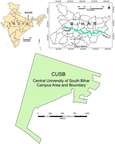
Figure 2. Bar diagrams showing area of a ground measured polygon under different map projections and datums and its comparison with ground measured (Y) of a polygon – a university campus from India.

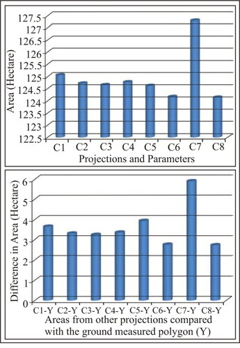
Table 1. Example of a ground measured area/polygon—The extent of area under different projections and parameters.

Projections and parameters	Area of the ground measured polygon (in ha/acres)
UTM Zone 44 with WGS 84 C1	125.0555 / 309.0185
UTM Zone 45 with WGS 84 C2	124.7171 / 308.1821
Polyconic with Everest 1969 Central Meridian (CM) 84.50 Latitude of Origin (LO) 13.00 C3	124.6517 / 308.0213
Polyconic with WGS 84 CM 82.50 / LO 16.00 C4	124.7677 / 308.3080
Lambert Conformal Conic (LCC) with WGS 84 LO 16.00 / CM 81.00 First Standard Parallel (FSP) 12.00 S Standard Parallel (SSP) 25.00 C5	124.6172 / 307.9359
LCC with WGS 84 FSP 13.00 / SSP 26.00 LO 16.00 / CM 82.50 C6	124.1676 / 306.8250
LCC with Everest 1969 FSP 13.75 / SSP 18.75 LO 16.25 / CM 80.87 C7	127.3017 / 314.5695
LCC with Everest 1969 FSP 13.00 / SSP 26.00 LO 16.25 / CM 82.50 C8	124.1394 / 306.7553

Table 2. Differences in area from other projections compared with the ground measured polygon.

Areas from other projections compared with the ground measured polygon Y = 121.4058 ha / 300 acres	Difference in area (ha / acres)	Percentage of difference compared with the ground measured polygon ‘Y’	Order of difference compared with the standard
C1 (125.0555) – Y	+3.6497 / 9.0185	+3.0061	7
C2 (124.7171) – Y	+3.3113 / 8.1827	+2.7275	5
C3 (124.6517) – Y	+3.2459 / 8.0212	+2.6727	4
C4 (124.7677) – Y	+3.3619 / 8.3079	+2.7693	6
C5 (124.6172) – Y	+3.9359 / 7.9359	+2.6453	3
C6 (124.1676) – Y	+2.7618 / 6.8250	+2.2750	2
C7 (127.3017) – Y	+5.8959 / 14.5695	+4.8565	8
C8 (124.1394) – Y	+2.7336 / 6.7553	+2.2517	1

4.2. Experiment with area of a polygon—case of the Ganga Basin

The boundary/perimeter of the Ganga River basin extends approximately between 21° 30′ N and 31° 45′ N Latitudes and between 73° E and 90° E Longitudes. The three UTM zones within which the Ganga river basin falls were given UTM projection with WGS 84 datum (separately for each of the three zones). Area of each of the polygons was then calculated (Figure 3 and Table 3). Similarly, the whole Ganga basin as a single polygon was given UTM projection with Zone 44 (the central zone of the Ganga River basin) and WGS 84 datum (Figure 3). The same process is repeated for the whole basin giving different projections with different parameters and datums (Table 3). When the area of the Ganga basin is split into 3 UTM zones with WGS 84 datum the resultant total area of all the three zones put together came to 1031082.7531326 sq. km. This is designated as ‘A1’ in Tables 3 and 4 and is taken here as a ‘standard’ as the deviations if any are expected to be minimal in UTM zones as each zone accounts for only 6° of longitude. Compared with this ‘standard’ area, the same Ganga River basin with Polyconic projection with Everest India-Nepal datum (the actual NSF suggested datum is Everest Modified) produced a larger area by 4384.195814 sq. km (A3 in Table 4). Similarly, with each case of other projections, parameters and datums (Table 3) the resultant area of the Ganga River basin has come to be larger than the ‘standard’.

Figure 3. Map showing the Ganga river basin with UTM 44 N zone and WGS 84 datum (top); parts of the Ganga basin with separate UTM zones – 43, 44 and 45 with WGS 84 datum (bottom).

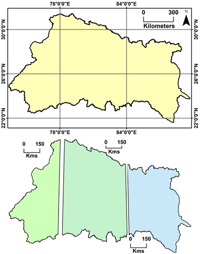
Table 3. Example of the Ganga Basin—The extent of area under different projections and parameters

Projections and parameters	Area of the Ganga River Basin (sq. km)
Universal Transverse Projection (UTM) 3 zones (43, 44 & 45) separately with World Geodetic System (WGS) 84 ‘Standard’ A1	1031082.7531326
UTM Zone 44 with WGS 84 A2	1035881.56566
Polyconic with India Everest India-Nepal Central Meridian (CM) 84.50 Latitude of Origin (LO) 13.00 (NRSC) A3	1035466.94894
Polyconic with WGS 84 CM 84.50 / LO13.00 A4	1035702.70884
Lambert Conformal Conic (LCC) with WGS 84 LO 16.253259 / CM 80.8749 First Standard Parallel (FSP) 24.50 Second Standard Parallel (SSP) 28.50 A5	1032687.21106
LCC with WGS 84 FSP 13.75 / SSP 18.75/ LO 16.253259 / CM 80.8749 A6	1065112.70181
LCC with Everest India-Nepal FSP 13.75 / SSP 18.75 LO 16.253259 / CM 80.8749 (NRSC) A7	1064871.92716
LCC with Everest India-Nepal FSP 24.50 / SSP 28.50 LO 16.253259 / CM 80.8749 A8	1032452.28527

Table 4. Differences in areas from other projections compared with ‘standard’ area. Example of the Ganga Basin.

Areas from other projections compared with the standard area (A1 = 1031082.7531326)	Difference in Area (sq. km)	Percentage of difference compared with the standard area ‘A1’	Order of difference compared with the standard
A2 (1035881.56566) – A1	4798.8125274	+0.46	5
A3 (1035466.94894) – A1	4384.1958074	+0.42	3
A4 (1035702.70884) – A1	4619.9557074	+0.45	4
A5 (1032687.21106) – A1	1604.4579274	+0.16	2
A6 (1065112.70181) – A1	34029.9486774	+3.30	7
A7 (1064871.92716) – A1	33789.1740274	+3.27	6
A8 (1032452.28527) – A1	1369.5321374	+0.13	1

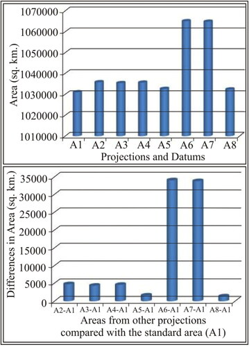
The area differences, the percentage of differences and the order of difference compared with the ‘standard’ area, are presented in Tables 3 and 4 and Figure 4. Projections A8 (+0.13%) and A5 (+0.16) came up with minimum positive differences from the standard (Table 4). The area differences from projections A4 (+0.45%), A3 (+0.42%) and A2 (+0.46%), though on the higher side from A8 and A5, fall in a group with insignificant differences from each other. Projections A7 (+3.27%) and A6 (+3.30%) are exceptions with very large differences from the ‘standard’. So, A8 and A5 with minimum differences from the ‘standard’, stand out as the best fit ones in this experiment (Table 4 and Figure 4).

Figure 4. Bar diagrams showing area of Ganga basin under different map projections and datums and its comparison with standard area (A1).

4.3 Experiment with area and shape of a polygon—case of whole India

In this experiment, whole of India including all its islands are taken as an example of a polygon. As in the case of the polygon of the Ganga Basin described above, the GIS shape file of India is cut into six polygons coinciding with six (Zones 42 to 47) UTM zones within which the area of India is covered (Figure 5) and were projected with UTM WGS 84 datum. Then, the area falling within each zone is separately calculated. The areal extent of all zones together covering India totalled up to 3232158.095668 sq. km (B1 in Table 5). This area (B1) is taken as the ‘standard’.

Figure 5. Map showing whole India with six UTM zones with WGS 84 datum.

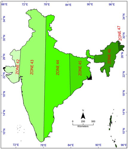
Table 5. Projections, parameters and resultant areas. Example of India.

Projections and parameters	Area of India (sq. km)
Universal Transverse Projection (UTM) 6 zones (42 to 47) separately with World Geodetic System (WGS) 84 ‘Standard’ B1	3232158.095668
UTM Zone 44 with WGS 84 B2	3296424.842714
Polyconic with Everest 1969 Central Meridian (CM) 84.50 Latitude of Origin (LO) 13.00 B3	3292646.392607
Polyconic with WGS 84 CM 82.50 / LO 16.00 B4	3286710.860431
Lambert Conformal Conic (LCC) with WGS84 LO 16.00 / C81.00 First Standard Parallel (FSP) 12.00 Second Standard Parallel (SSP) 25.00 B5	3285233.22112
LCC with WGS 84 FSP 13.00 / SSP 26.00 LO 16.00 / CM 82.50 B6	3276541.590867
LCC with Everest 1969 FSP 13.75 / SSP 18.75 LO 16.25 / CM 80.87 B7	3348620.532232
LCC with Everest 1969 FSP 13.00 / SSP 26.00 LO 16.25 / CM 82.50 B8	3275694.311204

Further, the same map of India referenced with UTM projection with Zone 44 and WGS 84 datum has given an area of 3296424.842714 sq. km. Also, the same map of India was given different projections with different data (datums) and parameters (Table 5), and the respective areas were calculated and presented in Table 5. It is interesting to note that in the case of entire India too, the areal extent compared with the so called ‘standard’ (B1), is greater in all cases of other projections (Table 6). Projection B7 is an exception with the largest difference of +3.47%. The pair of projections B6 (+1.35) and B8 (+1.32) make up one group with minimum difference. Projection B4 (+1.65) and B5 (+1.61) with insignificant difference between them is the second group with a moderate difference from the standard. The pair of projections B8 and B6 with minimum difference (Table 6 and Figure 6) prove to be best fit in this experiment.

Figure 6. Map projections and datums with respective areas of whole India and its comparison with standard area (B1).

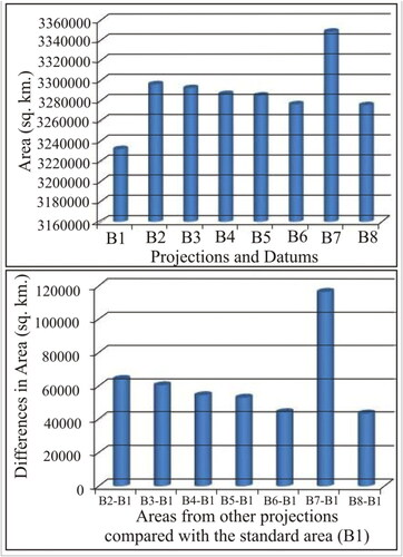
Table 6. Differences in areas from other projections compared with ‘standard’ area. Example of India.

Areas from other projections compared with the standard area (B1 = 3232158.095668)	Difference in area (sq. km)	Percentage of difference compared with the standard area ‘B1’	Order of difference compared with the standard
B2 (3296424.842714) – B1	64266.747046	+1.95	6
B3 (3292646.392607) – B1	60488.296939	+1.83	5
B4 (3286710.860431) – B1	54552.764763	+1.65	4
B5 (3285233.22112) – B1	53075.125452	+1.61	3
B6 (3276541.590867) – B1	44383.495199	+1.35	2
B7 (3348620.532232) – B1	116462.436564	+3.47	7
B8 (3275694.311204) – B1	43536.215536	+1.32	1

The areas of India map obtained under different projections (B1 to B8 in Tables 5 and 6) are compared with the official area of India (X in Table 7) (https://www.india.gov.in/india-glance/profile) (NPI, 2002) which is 3,287,263 sq. km (Table 7). A glance at Table 7 and Figure 7 reveals that projection B3 (+0.16%) has come up with minimum difference followed by B2 (+0.28%). With Projection B7 (+1.87%) the difference is relatively larger. On projections B1, B4, B5, B6 and B8 the calculated area of India came up lesser than ‘X’ the official area of India. Though the difference in area is on the negative side (Table 7 and Figure 7), there is almost a close match in areal extent between ‘X’ (3287263 sq. km) and ‘B4’ (3286710.86 sq. km) (Table 7). Projections B3 (+0.16%) and B4 (-0.0175%), with the former showing minimum positive difference and the latter showing minimum negative difference stand up as the best fit ones in this experiment.

Figure 7. Boundaries of maps with various projections and datums. Insets 1 to 3 are enlargements of segments (from inset blocks) of boundaries at different scales.

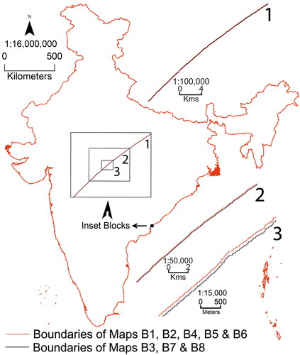
Table 7. Differences in areas from other projections compared with the official area of India.

Areas from other projections compared with the official area of India (X = 3287263 sq. km)	Difference in area (sq. km)	Percentage of difference compared with the official area of India ‘X’	Order of difference compared with the standard
B1 (3232158.095668 -- X	−55104.904332	−1.67	7
B2 (3296424.842714) – X	+9161.842714	+0.28	4
B3 (3292646.392607) –X	+5383.392607	+0.16	3
B4 (3286710.860431) – X	−552.139569	−0.017	1
B5 (3285233.22112) – X	−2029.77888	−0.06	2
B6 (3276541.590867) – X	−10721.409133	−0.33	5
B7 (3348620.532232) – X	+61357.532232	+1.87	8
B8 (3275694.311204) – X	−11568.688796	−0.35	6

To examine the shape differences, all the maps of India on projections B1 to B8, are composed together (Figure 7). It is interesting to note that there are no major differences of shape among the maps. Boundaries of maps B1, B2, B4, B5 and B6 superposed exactly one over the other and boundaries of maps B3, B7 and B8 coincided exactly with each other and finally both the groups show up as only two lines (Figure 7). And, the difference of shift in the boundaries between the two groups of maps in terms of distance is in the range of 0 to 100 m only. The shift in boundaries between the two groups can only be seen at larger scales starting from 1:100,000 (see insets in Figure 7).

5. Discussion and conclusions

As has been mentioned earlier, map projections depend upon the location of one’s area of interest over the globe. As far as India is concerned, polyconic projection had long been decided as the best projection because of minimum area error and shape distortion. In fact, in the case of India, zones-wise projection with UTM WGS 84 gives much accurate measurement of area than with polyconic or any other conical projections because the longitudes spread out wider towards the south in conical projections unlike in UTM zones. Lambert Conformal Conic projection too which is basically a conical projection is also suitable for India. As it is, UTM projection is unsuitable for India as India falls in six UTM zones. In such a case, though theoretically the area measurements (of a large area within 20° of latitudinal width range), can be much more accurate than with polyconic projection, there will be problem of combining and merging data of different UTM zones. That means, though strips of maps of adjoining UTM zones can be mosaicked together but cannot be merged as each zone has a different origin and parameters. So, geospatial information generated by various individuals and organizations for areas falling in different UTM zones cannot be brought together in a single data frame for many operations in GIS software. This difficulty forecloses the use of UTM projection to generate geospatial data in case of India. But, still, several spatial data creators including several governmental organizations use UTM projection with WGS 84 datum to be one with the rest of the world (as UTM with WGS 84 is a very popular projection worldwide) and geo-reference the data (of large areas within India and of whole India) with UTM WGS 84 projection by using parameters of UTM Zone 44 (in Indian case). Here, in the present experiment, it has been observed that area calculated separately zones-wise (3232158.095668 sq.km) is less than the official area of India (X = 3287263 sq. km in Table 7). The difference (9161.84 sq. km accounting for 0.28%) between the official area of India (3287263 sq. km - X in Table 7) and the area of India with UTM Zone 44 projection (3296424.84 sq. km - B2 in Table 7) is not significant and it is a little more (not less) than the official area of India (Table 7).

As has been mentioned in data and methodology, the percentage of differences from the ‘standard areas’ are given scores in increasing order starting from 1 for the minimum with maximum difference going up to 8 (Tables 2, 4, 6 and 7) and all the scores for similar projections are added up to prepare ranks (Table 8). It is to be noted here that projections designated A1 to A8 are similar to B1 to B8 and C1 to C8. Finally, based on ranks (Table 8) A8, B8, C8; A5, B5, C5; A3, B3, C3; A4, B4, C4 are selected as the best fit projections with minimum differences from the ‘standard’ areas.

Table 8. Order of differences in area compared with the standard of the three experiments—the Ganga River basin, India, and the ground measured area and final ranks based on differences.

Projections from Tables 1, 3 and 5	Ganga River Basin from Table 4	India		Ground measured area from Table 2	Total score from tables 2, 4, 6and 7	Rank based on differences
		From Table 6	From Table 7
C1 A1 B1	---	---	7	7	--	---
C2 A2 B2	5	6	4	5	20	5
C3 A3 B3	3	5	3	4	15	3
C4 A4 B4	4	4	1	6	15	3
C5 A5 B5	2	3	2	3	10	2
C6 A6 B6	7	2	5	2	16	4
C7 A7 B7	6	7	8	8	29	6
C8 A8 B8	1	1	6	1	09	1

If the states go with their local parameters and other national institutions go with all-India parameters, there would be a problem of compatibility in putting together different sets of geospatial data. Whether it is local or national, it is advisable to implement a single all-India projection with common parameters so that there is data compatibility which facilitates all India mosaic in a single data frame. All funding organizations dealing with any kind of spatial data generation should insist on a common projection with common parameters so that there is data compatibility between the data sets. As for shape of India under various projections with various parameters (Tables 6 and 7 and Figure 7), there is no significant distortion at all (maximum 100 m of shift with minimum being zero). Finally, based on ranks (Table 8) the authors suggest (i) LCC with Everest India-Nepal datum (A8, B8, C8), (ii) LCC with WGS 84 datum (A5, B5, C5), (iii) Polyconic with Everest 1969 datum (A3, B3, C3), and (iv) Polyconic with WGS 84 datum (A4, B4, C4), both for mapping smaller areas on larger scales (excluding cadastral maps) and larger areas on smaller scales, as the best fit ones in case of India. The difference in extent of areas from the ‘standard’ increase from (i) to (iv). In all the studies, quoted in the paper, conducted for different areas outside India, there were variations obviously in extent of area and they suggested/used best fit projections based on minimum area differences after comparing their results with either ground measured areas or available official areas.

References

- Al Hameedwani ANM. 2018. Comparing the accuracy of different map projections and datums using truth data. J Univ Babylon Eng Sci. 26(4):18–32.
- Danielsen J. 1989. The area under the geodesic. Surv Rev. 30(232):61–66.
- Ghosh JK, Dubey A. 2008. India’s new map policy – utility of civil users. Curr Sci. 93(3):332–337.
- Ghosh JK, Dubey A. 2009. Imapct of India’s new map policy on accuracy of GIS theme. J Indian Soc Remote Sens. 37(2):215–221.
- Gillissen I. 1993. Area computation of a polygon on an ellipsoid. Surv Rev. 32(248):92–98.
- GitHub. 2002. Datameet/maps: repository for all spatial data. [Accessed 2022 January 30]. https://github.com/datameet/maps.
- Kennedy M, Kopp S. 2000. Understanding map projections. Redlands, USA: Environmental Systems Research Institute; p. 1–116.
- Kimerling JA. 1984. Area computation from geodetic coordinates on the spheroid. Surv Mapp. 44:343–351.
- Krejčí J. 2008. Methods for georeferencing early maps. Bull Soc Cartograph. 42:45–48. https://maps.fsv.cvut.cz/gacr/publikace/2009/2009_Krejci_SOC.pdf.
- Lapaine M, Usery EL, editors. 2017. Choosing a map projection. Gewerbestrasse, Cham, Switzerland: International Cartographic Association.
- Mailing DH. 1992. Coordinate systems and map projections. 2nd ed. Exeter, United Kingdom: Pergamon Press.
- Misra I, Rohil MK, Moorthi SM. & Dhar, D. 2022. A novel country-level integrated image mosaic system using optical remote sensing imagery. Earth Science Informatics. 15(4):2181–2193.
- National Map Policy. 2005. Survey of India, Department of Science and Technology, New Delhi. [Accessed 2021 September 25]. https://surveyofindia.gov.in/documents/national-map-policy.pdf.
- National Portal of India. 2022. [Accessed 2022 January 30]. https://www.india.gov.in/india-glance/profile.
- Pearson F. 1990. Map projections: theory and applications. 2nd ed. Boca Raton, USA: CRC Press; p. 1–388.
- Seong JC, Mulcahy KA, Usery EL. 2002. The sinusoidal projection: a new importance in relation to global image data. Prof Geogr. 54(2):218–225.
- Sjöberg LE. 2006. Determination of areas on the plane, sphere and ellipsoid. Surv Rev. 38(301):583–593.
- Usery EL, Finn MP, Cox JD, Beard T, Ruhl S, Bearden M. 2003. Projecting global datasets to achieve equal areas. Cartogr Geogr Inform Sci. 30(1):69–79.
- Usery EL, Seong JC. 2000. A comparison of equal-area map projections for regional and global raster data. In: Proceeding of 29th International Geographical Congress, Seoul, Korea.
- Yang Q, Snyder JP, Tobler WR. 1999. Map projection transformation, Principles and Applications. 1st ed. london, UK: Routledge, CRC Press, Taylor and Francis. p. 1–388.
- Yıldırım F, Kaya A. 2007. Equal-area projections on GIS and ArcGIS applications. In: Proceeding of TMMOB Geographical Information Systems Congress, Karadeniz Technical University, Trabzon, Turkey (in Turkish).
- Yildirim F, Kaya A. 2008. Selecting map projections in minimizing area distortions in GIS applications. Sensors (Basel). 8(12):7809–7817.