Toward the automatic detection of effective gerbil holes in desert grasslands through unmanned aerial vehicle imagery

Abstract

Rapidly determining the density of effective gerbil holes is ecologically important but technically challenging. However, unmanned aerial vehicles (UAVs) offer new methods to identify effective gerbil holes and understand the spatial relationships between gerbils and grass coverage. In this study, we focused on Meriones unguiculatus, which live in desert grasslands of Ordos, and gathered UAV imagery to explore the performance of rule-based classification in object-based image analysis (OBIA) for identifying effective gerbil holes. To improve the classification accuracy and reduce the time cost of repeated ‘trial and error’, we propose a novel method to build rule sets. We adopted the estimation of scale parameter_2 (ESP2) method during the segmentation stage to enable fast and objective segmentation parameterization. For the classification stage, a correlation-based feature selection (CFS) algorithm was applied for feature selection and threshold prediction. Our analysis determined the following universally recommended rule sets for identifying effective gerbil holes using OBIA: scale parameter of 107, shape factor of 0.2, compactness value of 0.3, excess green value less than −5, brightness feature value in the 143–149 range and roundness feature less than 0.9. With these rule sets, OBIA exhibited higher classification accuracy than maximum likelihood (ML) classification, with an overall classification accuracy of 88.25%. We also found that the relationship between the area of effective gerbil holes (y) and the grass coverage (x) satisfied a quadratic function:$y=-1.981x^2+1.104x\text{+}0.416.$ This study provides practical guidance for grassland management and rodent infestation control.

Keywords:

• Effective gerbil holes
• UAV imagery
• OBIA
• CFS

1. Introduction

Inner Mongolia is home to the largest grassland in China, but severe and very severe desertification has affected a significant portion of the region, with 98% of desertification occurring in grasslands (Kang and Liu 2014; Guo et al. 2015). Despite efforts to control desertification over the past 50 years, the overall trend has not improved substantially (Wei and Fang 2009; Guo et al. 2014). Rodent populations have increased as a concomitant phenomenon of grassland desertification, leading to the destruction of bare soil structures, interruption of material and energy flow and exacerbation of the process of grassland desertification (Lü et al. 2016; Tang et al. 2019). Rodents also gnaw on forage, reducing plant diversity (Chen et al. 2017). Mongolian gerbils (Meriones unguiculatus) are the hosts of the plague, and there has been a resurgence of plague outbreaks in the past seven years, with a direct correlation between outbreaks and the increased density of M. unguiculatus (Davis et al. 2008; Eads et al. 2016; Feng et al. 2020). Monitoring the density and distribution of gerbil populations, indicated by the number and area of effective gerbil holes, is crucial for grassland management and plague prevention and control (Liu et al. 2019).

To carry out rodent censuses, the traditional method is to count effective gerbil holes using ground-based field surveys. However, this method is laborious, lacks spatial information and carries a risk of acquiring plague infection. Additionally, existing data gaps for harsh environments further limit the accuracy of traditional methods (Tang et al. 2019). With the development of geospatial technologies, remote sensing has become an increasingly popular method to monitor rodent populations (He et al. 2013; Chen et al. 2017). Related studies have used the spectral characteristics of rodent hazard areas to estimate population density (Liu et al. 2013; Pang and Guo 2017). However, the low spatial resolution data used in these studies limits the efficiency of monitoring rodent population density.

In recent years, remote sensing has advanced significantly toward generating and applying high temporal and spatial resolution data (Bhardwaj et al. 2016; Van Cleemput et al. 2018). UAVs have been widely used in ecological research due to their ability to provide high-resolution data. For example, Dandois and Ellis (2013) used UAVs to monitor plant phenology in a 50 m × 50m sample plot in Maryland, USA, while Sun et al. (2018) integrated UAV technology with a deep learning framework to extract pest areas in forest monitoring. The use of UAVs in animal behavior and population surveys has also attracted the attention of animal ecologists. Weissensteiner et al. (2015) used UAVs to assess the breeding behavior of birds and compared it to traditional survey methods, saving 85% of time. Rey et al. (2017) proposed a semi-automatic system with UAVs to detect animals in savannas and achieved 75% correct detection for a precision of 10%. In the field of environmental protection, Wu et al. (2020) used color features to recognize residual plastic film from UAV images, providing a decision-making basis for farmland environmental health assessment. Pi et al. (2021) constructed a low-altitude UAV platform and achieved high-precision classification of desertification degradation indicator plants, providing quantitative data for developing ecological restoration.

However, achieving high accuracy with high-resolution remote data has been challenging due to the heterogeneity in local pixel values and spectral similarities among different types of data. Processing remote sensing data with pixels as primary mapping units also poses a challenge (Dronova 2015; Ma et al. 2017a).

Object-based image analysis (OBIA) provides a solution for analyzing high-resolution images by offering meaningful semantic information and spatial characteristics between neighboring pixels (Drăguţ et al. 2010; Juan et al. 2017; Ma et al. 2021a, 2021b). Previous research on OBIA has focused on land-cover (Costa et al. 2014; Tehrany et al. 2014) and wetland (Dronova 2015) projects and the methods used are primarily based on decision trees (Laliberte et al. 2006; Mallinis et al. 2008), the K-nearest-neighbors algorithm (Tehrany et al. 2014; Ma et al. 2017b) and artificial neural networks (Marmanis et al. 2016; Zhou and Han 2021). However, the accuracy of these supervised classification methods is limited by data sources, training set size and segmentation parameters (Ma et al. 2017a; Chen et al. 2018). Additionally, selecting representative samples for each category is time-consuming and laborious and can result in significant human error. In contrast, unsupervised algorithms (Langner et al. 2014; Ma et al. 2014; Charoenjit et al. 2015) provide an automatic and flexible approach to remote sensing image classification by obtaining information from the spectrum, texture and geometry. Rule-based algorithms, as a representative of this approach, usually suggest an optimal parameter and require a threshold (Espindola et al. 2006; Johnson and Xie 2011; Dronova 2015) to perform unsupervised classification (Langner et al. 2014), which can be applied to a large amount of data from the same batch of flights, enabling real-time data processing.

Previous researches on rule-based algorithms for classification mostly dependent on subjective ‘trial and error’ methods, this leaded to uncertainty in classification accuracy (Johnson and Xie 2011; Belgiu and Drǎguţ 2014). ESP2 tool have been developed to promote automatic decision on segmentation specifications (Liu and Ren 2022). Related studies have shown that unsupervised segmentation based on ESP2 are, in contrast, less subjective and more time-efficient, making them suitable for use in operational remote imagery classification settings (Drăguţ et al. 2010, 2014). Due to high-resolution remote sensing data provide more detailed information, there are more than 200 features per object after segmentation (Laliberte et al. 2012). The large number of features not only causes difficulties in the establishment of classification rules, but also easily leads to dimensional disasters. Feature selection enables to obtain data for comprehensive understanding of objects (Pal and Foody 2010), and, to identify representative features and make predictions about their thresholds (Ma et al. 2017a), has become an important process to improve classification accuracy and enhance classification efficiency. Ma et al. (2015) applied CFS method to implement dimensionality reduction of the object features prior to classification, and proposed that CFS is the optimal feature selection algorithm in OBIA. The related studies on feature selection have been conducted in supervised classification methods of OBIA. Thus, there are few research on rule-based algorithms classification in the OBIA field, and, there is no common consensus about the general effects of the combination of feature selection methods and unsupervised rule-based classification.

The main objective of this study is to develop a rule set for object-based unsupervised classification instead of relying on supervised classification methods in OBIA. To achieve this, we combined automatic segmentation scale estimation in multiresolution segmentation with the CFS method to predict segmentation parameters and feature threshold values. Our study focuses on the meaningful visual characteristics of effective gerbil holes in desert grasslands, building on previous OBIA research. To the best of our knowledge, this study is the first to use UAV imagery to identify effective gerbil holes, and the findings are essential for understanding high-resolution data in specific applications.

2. Materials and methods

2.1. Study area

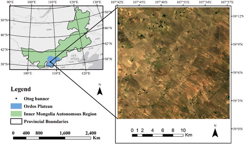
This study was conducted at Otog Banner (39°25'N, 107°58'E), Ordos Plateau. The Ordos Plateau is located southwest of the Inner Mongolia Autonomous Region, China, which is a typical representative area of the desert grassland of Inner Mongolia, with an approximate elevation of 1300 m (Figure 1). The mean annual temperature is 9.6 °C, and the annual precipitation is approximately 237.4 mm, but the annual average evaporation is up to 2470 mm. The surface bare soil is mainly light chestnut and brown calcium bare soil, with a large sand content and poor loose nutrient characteristics (Liu et al. 2019). Otog Banner is one of the plague natural focuses of M. unguiculatus on the Inner Mongolian Plateau.

Figure 1. Location of the study area on Ordos Plateau, China.

2.2. Acquisition of UAV imagery and sample selection

In this study, we collected aerial images of five sample plots with different densities of effective gerbil holes in April 2020 and April 2021. Each sample plot covered an area of 50 m × 50 m. Table 1 provides information on the geographical distribution of the sample plots and the statistics of effective gerbil holes obtained through ground surveys. We used quadrotor M200 UAVs (DJI-Innovations, Shenzhen, China) as the data acquisition platform and selected clear and cloudless days from 12:00 to 14:00 to minimize the impact of shadows on the classification results. The altitude was set to 30 meters, and the forward and side overlaps were set to 70% and 80%, respectively. A total of 445 images were collected, with each sample plot having 89 images of size 5280 pixels × 3956 pixels. We used Pix4D (https://www.pix4d.com/), a professional drone mapping software, to correct and mosaic the images and generate digital orthophoto maps (DOMs) with a resolution of 0.4 cm.

Table 1. Sample plots distribution and the numbers of gerbil holes.

Sample plot number	Longitude (/°)	Latitude (/°)	Number of effective gerbil hole
1	107.9353338	39.37637958	78
2	107.3285293	39.74653606	105
3	107.3461522	39.67427311	71
4	107.4647808	38.68700939	25
5	107.5344532	39.24878197	112

The images were captured during the herbage re-greening period, when the leaves of forage were green, and the effective gerbil hole patches were clearly distinguishable from the grassland in terms of texture and color. The images also contained a significant amount of bare soil and a few black patches, which were formed by withered grass shadows and abandoned gerbil holes. However, these black patches did not affect the extraction of effective gerbil hole information. We classified the ground objects in the UAV imagery into three categories: grass patches, effective gerbil holes and soil patches.

To determine a universally applicable threshold for the extraction of effective gerbil holes, we randomly selected 60 object samples from each sample plot (20 from each category) for a total of 300 samples. We used 60% of the samples for training and the remaining 40% for testing. We created raster files of all the object samples in eCognition, and then, converted them into polygons using ArcGIS as the regions of interest (ROIs) for the maximum likelihood (ML) classification.

2.3. Segmentation scale estimation using ESP2

OBIA considers both spectral and morphological, contextual and proximity features in images; therefore, many previous studies have indicated that the OBIA method outperformed pixel-based classification in very-high-resolution images (Blaschke 2010; Zhu et al. 2020; Luo et al. 2021). The OBIA consists of two main function modules: image segmentation and target object extraction (Addink et al. 2007). Image segmentation is a process of dividing remote sensing images into discrete regions or objects that are homogeneous in terms of spatial or spectral characteristics. This process reduces the within-class spectral variation in the high spatial resolution imagery and the fragmentation rate of the object (Jing and Cheng 2012). The OBIA in this study is performed using eCognition Developer 64 software, which is the world’s first object-based classification software (Drăguţ et al. 2010, 2014).

The commonly used segmentation methods in eCognition Developer include the chessboard, quadtree, contrast, multiresolution, spectral difference, multithreshold and contrast filter segmentation methods. Among them, multiresolution segmentation, which uses the region-growing segmentation algorithm, is the most effective segmentation method for acquiring information at different scales (Zhang et al. 2010; Mengmeng and Noboru 2017). For multiresolution segmentation, the most critical procedure is to choose appropriate segmentation parameters (typically containing scale parameters, shape factors and compactness values) to increase the interclass spectral differences of images and improve the accuracy of classification and identification (Addink et al. 2007). However, it is challenging to define the optimal segmentation parameters for image objects of different sizes and shapes in different scenes of remote sensing data (Meinel and Neubert 2004). OBIA correlates the segmentation parameters of images with spatial attributes and constructs a mean variance (Eq. (1)(1) $$L{V}_k^{}=\frac{1}{m}\times \sum _{}^{}(\frac{1}{n}\times \sum _{i=1}^n{C}_{ki}-\frac{1}{n\times m}\times \sum _{i=1}^{n\times m}{C}_{ki}{)}^2$$(1) , Woodcock and Strahler 1) based on the segmentation objects to evaluate the merits of the scale parameters.

The ESP2 tool (an eCognition plug-in) evolved on the mean variance, iteratively generated image objects at multiple scale levels in a bottom-up approach, and measured LV (local variance) as the values of mean variance in a 3 × 3 moving window, while extending the calculation of local variance from one band to multiple bands (Eq. (2)(2) $$LV=(L{V}_1+L{V}_2+\dots ,+L{V}_k+\dots ,+L{V}_l)/l$$(2) ). (1) $$L{V}_k^{}=\frac{1}{m}\times \sum _{}^{}(\frac{1}{n}\times \sum _{i=1}^n{C}_{ki}-\frac{1}{n\times m}\times \sum _{i=1}^{n\times m}{C}_{ki}{)}^2$$(1) where $L{V}_K$ is the mean variance of different objects in band k, $C_{ki}$ is the luminance value of the $i$ th pixel in the object in band k, n is the number of pixels in an object and m is the total number of objects in an image. (2) $$LV=(L{V}_1+L{V}_2+\dots ,+L{V}_k+\dots ,+L{V}_l)/l$$(2) $L{V}_{}$ is the mean value of $L{V}_K$ over l bands. The dynamic change in $L{V}_{}$ reveals the effect of segmentation from one object level to another. To show the dramatic degree of change, the rate of change ($\mathit{ROC},$ Eq. (3)(3) $$\mathit{ROC}=\left[\frac{L-(L-1)}{L-1}\right]\times 100$$(3) ) is defined in ESP2. The thresholds in the rates of change indicate the scale levels at which the image can be segmented in the most appropriate manner relative to the data properties at the scene level. (3) $$\mathit{ROC}=\left[\frac{L-(L-1)}{L-1}\right]\times 100$$(3) where $L=LV$ at the target level, and $L-1=LV$ at the next lower level. $\mathit{ROC}-L{V}_{}$ measures the amount of change in $L{V}_{}$ from one object level to another, the local maximum in the $\mathit{ROC}-L{V}_{}$ graph indicate the object levels at which the image can be segmented in the most appropriate manner.

The ESP2 tool is programmed in Cognition Network Language (CNL) in the eCognition Developer 64 software (Tiede and Hoffmann 2006), and it is implemented as a customized process to be applied easily similar to other processes in object-based rule set creation in the Definiens software. Six user-defined parameters are adjustable: (1) step size of increasing scale parameter, (2) starting scale parameter for the analysis, (3) the use of an object hierarchy during segmentation, (4) number of loops (i.e. number of scales to be tested), (5) shape weighting and (6) compactness weighting. Parameters (5) and (6) are used as implemented in multiresolution segmentation (Benz et al.2004; Zhu et al. 2020). The simple yet robust ESP2 tool enables fast and objective parametrization when performing multiresolution segmentation.

2.4. Correlation-based feature selection technique

In contrast to other dimensionality reduction techniques, such as those based on projection (e.g. principal component analysis) or compression, feature selection techniques do not alter the original representation of the variables but merely select a subset of them. Thus, they preserve the original semantics of the variables, thereby providing a visual characterization of the features (Espindola et al. 2006).

The CFS assessed the worth of a set of features using a heuristic evaluation function based on the correlation of features, and Hall and Holmes (2003) claimed that a superior subset of features should be correlated with classes highly uncorrelated to each other. Thus, the criteria for a feature subset containing k features can be evaluated using the following formula (Eq. (4)(4) $$\text{merit}=\frac{k\overline{r_{cf}{}_{}}}{\sqrt{k+k(k-1)\overline{r_{ff}{}_{}}}}$$(4) ). (4) $$\text{merit}=\frac{k\overline{r_{cf}{}_{}}}{\sqrt{k+k(k-1)\overline{r_{ff}{}_{}}}}$$(4) where f indicates the feature, c is the class, r is the Pearson correlation coefficient calculated by Eq. (5)(5) $$p(X,Y)=\frac{\sum _{i=1}^n(X_i-\overline{X})(Y_i-\overline{Y})}{\sqrt{\sum _{i=1}^n{(X_i-\overline{X})}^2}\sqrt{\sum _{i=1}^n{(Y_i-\overline{Y})}^2}}$$(5) (Hall 2000), $\overline{r_{cf}}$ denotes the mean feature correlation with classes, $\overline{r_{ff}}$ indicates the average feature intercorrelation and k denotes the number of attributes in the subset. In addition, the forward search was used to explore the feature space, and the search stop criterion was set when the heuristic takes three consecutive declines to avoid searching the entire feature space. In this study, Numerical Python was used to implement this feature selection algorithm. (5) $$p(X,Y)=\frac{\sum _{i=1}^n(X_i-\overline{X})(Y_i-\overline{Y})}{\sqrt{\sum _{i=1}^n{(X_i-\overline{X})}^2}\sqrt{\sum _{i=1}^n{(Y_i-\overline{Y})}^2}}$$(5) where X and Y represent two different feature vectors or a feature vector X and a target category Y. As shown in Algorithm 1, the CFS technique consists of feature preprocessing and feature selection.

Algorithm 1

Process of Correlation-based Feature Selection

Feature preprocessing

1: Sample labeling (Perform nearest neighbor algorithm and manual editing)

2: Select training samples

3: Export the features of objects X  Characteristic category is shown in Table 2

Table 2. Image object information on brightness, spectral and geometric features.

Characteristic category	Main content	Main application
Spectral	Mean blue, mean green, mean red, max difference, Standard deviation (std. dev.) blue, std. dev. green, std. dev. red, brightness, EXG (Vegetation indices of excess green index)	Spectral features were the most basic features for evaluating an image object’s pixel value.
Texture	GLCM (Gray-Level Co-occurrence Matrix) homogeneity in all directions, GLCM in the 0° direction, GLCM in the 45° direction, GLCM in the 90° direction, GLCM in the 135° direction	Texture features are derived from texture after Haralick based on the Gray-Level Co-occurrence Matrix or Gray-Level Difference Vector.
Geometric	Area, Width, border length, length/thickness, length/width, number of pixels, thickness, volume, width, asymmetry, border index, compactness, density, elliptic fit, roundness, shape index	Geometric features refer to the geometric information of meaningful objects, which is crucial to the classification effect when the target object has a regular geometry.

4: Calculate the variance of each feature separately ${\sigma }_i^2$

5: if ${\sigma }_i^2\le 0.05,$ eliminate this feature from X (Remove zero-difference feature)

Features selection

6: Create self._relevant_cols = [ ]

7: Create self._merit = None

8: The dimension of samples is n

9: for i in range(n):

10:   cor_relations = np.corrcoef(X,Y)

11:   correlations = cor_relations[:-1, :]

12:   max_index = np.argmax(correlations)

13:   self._relevent_cols.append(max_index)

14:   self._merit = correlations[max_index]

15: while True:

16:  for i in range(n):

17:    if i not in self.relevent._cols:

18:    $\overline{r_{ff}}$= cor_relations[row, col]

29:    $\overline{r_{cf}}$=cor_relations[tmp_relavent, −1].mean

20:    k =len(tmp_relavent)

21:    merit = (k*$r_{fc}$)/np.sqrt(k + k*(k-1)* $r_{ff}$)

22:  if merit > = max_merit:

23:    max_merits = merit

24:    return self._metrit

25:    return self._relavent_cols

2.5. Maximum likelihood classification

ML classification is a widely used supervised image classification method. It constructs classification functions by assuming the distribution of remote sensing data to a multidimensional normal Eq. (6)(6) $$P(\text{X|}{\theta }_i)\text{=}\frac{1}{2{\pi }^{\raisebox{1ex}{$k$}\!\left/ \!\raisebox{-1ex}{$2$}\right.}{\left|{\Sigma }_i\right|}^{\raisebox{1ex}{$1$}\!\left/ \!\raisebox{-1ex}{$2$}\right.}}\exp \hspace{0.17em}\left[-\frac{1}{2}{(\mathrm{X}-{\mu }_i)}^T{(\Sigma )}_i^{-1}(\mathrm{X}-{\mu }_i)\right]$$(6) (Lu et al. 2014). (6) $$P(\text{X|}{\theta }_i)\text{=}\frac{1}{2{\pi }^{\raisebox{1ex}{$k$}\!\left/ \!\raisebox{-1ex}{$2$}\right.}{\left|{\Sigma }_i\right|}^{\raisebox{1ex}{$1$}\!\left/ \!\raisebox{-1ex}{$2$}\right.}}\exp \hspace{0.17em}\left[-\frac{1}{2}{(\mathrm{X}-{\mu }_i)}^T{(\Sigma )}_i^{-1}(\mathrm{X}-{\mu }_i)\right]$$(6) where $p(\mathrm{X}|{\theta }_i)$ is the probability that a pixel X belongs to a class ${\theta }_i.$K is the number of bands, then $\text{X = [}{x}_1\text{, }{x}_2\text{, }\dots \text{, }{x}_k\text{]},$ ${\Sigma }_i$ and ${\mu }_i$ are the covariance matrix and mean value of class ${\theta }_i,$ respectively (Shi and Xue 2017).

The ML classification method calculates the distribution function of each class by extracting the mean and variance characteristics of the region of interest (ROI) and then estimating the probability of a pixel belonging to a particular class. Due to its ability to handle non-symmetric class distributions in the spectral domain, the ML method usually achieves high accuracy when the training data have high resolution (Richards 2006; Yang et al. 2011; Tian et al. 2013). In this study, we employed ENVI software to perform ML classification.

2.6. Process of identification of effective gerbil holes

This study proposes a fast and automatic system for identifying effective gerbil holes using UAV imagery. The system consists of three main steps, as illustrated in Figure 2:

Figure 2. Process of gerbil hole identification and optimization based on UAV imagery.

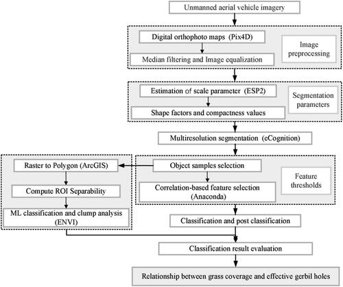
1. Preprocessing is performed on all samples to ensure the relative consistency of the initial features of all samples, and the spatial distribution of the desert grassland features is obtained.

2. Training is performed on samples to obtain a set of thresholds or parameters that define the meaningful visual characteristics of effective gerbil holes.

3. The validity and accuracy of the method are tested and evaluated on the test samples. To compare the classification results, typical pixel-based ML classification is used to classify the UAV imagery. The details of the system are described in Figure 2.

3. Results

3.1. Segmentation results

3.1.1. Scale parameters

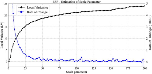
The scale parameter is the most critical segmentation parameter of multiresolution segmentation, as it directly affects the segmentation of the entire image. Figure 3 shows the changes in LV and ROC with increasing scale parameters. As the scale parameter grew from a single pixel (starting scale is 1) in steps of 2, LV gradually increased until it matched the objects in UAV imagery. Thereafter, as the scale parameter continued to increase, the boundary information of the object was retained at a higher segmentation level, while the LV value remained at the level indicating a meaningful ground object. ROC followed an opposite trend to LV. This trend revealed how fast the change in LV was in the transition from pixels to the smallest characteristics in the image. In the scale range of 20–40 intervals, the ROC decreased abruptly, indicating that there were no objects of interest with scales less than 40. The local peaks in the ROC curve theoretically represented the emergence of larger homogeneous objects as the scale increased and indicated the appropriate parameters for image segmentation. However, the variation induced by the background segmentation also generated peaks, making the graph interpretation complicated. We selected the most dominant peaks that were clearly separated from their neighborhood as indicators for optimal scale parameters, namely, 45, 93, 107, 153 and 173.

Figure 3. ESP tool outputs for the UAV imagery Graphs depict changes in local variance (LV) (solid black) and rate of change (ROC) (solid blue) with increasing scale parameter.

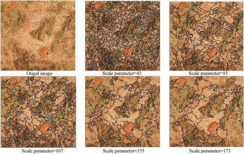
The segmentation results are shown in Figure 4, displaying significant differences between the different scale parameters. When the scale parameter was set to a small value (e.g. 45, 93), the characteristic difference of the target object (gerbil holes) was strongly influenced. Conversely, when the scale parameter was set too large (e.g. 153, 173), the image segmentation was relatively coarse, and the gerbil hole boundaries were low. Additionally, other grassland ground objects around the gerbil holes were incorporated into the target object. After continuous adjustment in the training set, we found an optimal scale parameter of 107 that showed a clear separation between bare soils, grassland and gerbil holes.

Figure 4. Segmentation results of UAV imagery under different scale parameters.

3.1.2. Shape factors and compactness values

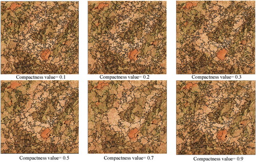
The shape factor represents the weight of the shape in homogeneity, and the sum of its value with that of the color factor is 1.0, determining the boundary fit for the image object. When optimizing the shape factor, iterative adjustments were made on the training set with the optimal scale parameter of 107. We found that the degree of coincidence of the gerbil hole boundary first increased and then decreased with increasing shape parameter. A small shape factor allowed for a greater influence of the color feature on the segmentation results, while a larger shape factor reduced the spectral homogeneity inside the gerbil holes, causing some of the gerbil holes to be incorrectly grouped with the bare soil. To further refine the object generation, compactness and smoothness values were calibrated. Lower weights on compactness (e.g. 0.1 or 0.2) increased the smooth factor and segmented more objects with linear shapes, which facilitated the extraction of grass patches. Conversely, a higher compactness parameter (e.g. 0.5 or 0.7) increased the compactness of the object and decreased the smoothness, leading to a poor fit of the effective gerbil hole edges. After repeated adjustments and visual assessments on the training set, we found that a shape factor of 0.2 and a compactness value of 0.3 resulted in an obvious separation between bare soil, grass and effective gerbil holes (as shown in Figures 5 and 6).

Figure 5. Segmentation results of gerbil holes under different shape factors.

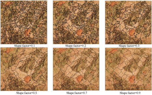
Figure 6. Segmentation results of gerbil hole under different compactness values.

3.2. Object-based classification result

To identify gerbil holes, the information of features is summarized and generalized to obtain feature thresholds for different ground objects, which is a key step in rule-based classification in OBIA. However, the large number of derived features per segmented object can lead to a time-consuming and subjective process of optimizing the feature subset (Ho and Rao 2016). The CFS method provides an algorithmic way to optimize feature subsets, and the visualization tool can make predictions about their thresholds of representative features.

3.2.1. Feature selection result

In the present study, 35 features were calculated for each object, including spectral, texture and geometry features. As the vegetation index was not defined in eCognition Developer, we created the excess green value (EXG, Eq. (7)(7) $$\mathit{EXG}=2\times G-R-B$$(7) ) (Toomey et al. 2015; Ran et al. 2016) to characterize the spectral features of vegetation. The details of all features are given in Table 2. After the univariate filtering method in feature preprocessing, two features, length_thic and thickness, were eliminated, leaving a final number of 33 valid features. The feature subsets ${\text{merit}}_{}$ obtained during traversal according to Eqs. (5)(5) $$p(X,Y)=\frac{\sum _{i=1}^n(X_i-\overline{X})(Y_i-\overline{Y})}{\sqrt{\sum _{i=1}^n{(X_i-\overline{X})}^2}\sqrt{\sum _{i=1}^n{(Y_i-\overline{Y})}^2}}$$(5) and (6)(6) $$P(\text{X|}{\theta }_i)\text{=}\frac{1}{2{\pi }^{\raisebox{1ex}{$k$}\!\left/ \!\raisebox{-1ex}{$2$}\right.}{\left|{\Sigma }_i\right|}^{\raisebox{1ex}{$1$}\!\left/ \!\raisebox{-1ex}{$2$}\right.}}\exp \hspace{0.17em}\left[-\frac{1}{2}{(\mathrm{X}-{\mu }_i)}^T{(\Sigma )}_i^{-1}(\mathrm{X}-{\mu }_i)\right]$$(6) are shown in Table 3. Although the available feature space for each object reached 35, there is a large amount of redundant information among them, and some are not related to the target class. For example, the correlations between max_diff and mean_r, mean_g and mean_b are as high as 0.93, 0.94 and 0.74, respectively. The correlation between roundness and elliptic_f, density, and rectangularity is greater than 0.9. With the extended feature space, OBIA may increase the complexity of the classification and the demand for computing power (Li et al. 2016). According to the CFS algorithm (Algorithm 1), the final optimal feature subset was determined, which contains the EXG, gray-level co-occurrence matrix (GLCM) and roundness. (7) $$\mathit{EXG}=2\times G-R-B$$(7) where R, G and B represent the pixel values of the red, green and blue bands, respectively.

Table 3. Correlation-based forward search process.

Feature subset	k	$\overline{r_{cf}}$	$\overline{r_{ff}}$	Merit
[ ]	0	N/A	N/A	0.0
[EXG]	1	0.751	1.000	0.751
[Brightness]	1	0.542	1.000	0.542
[GLCM]	1	0.420	1.00	0.420
[Roundness]	1	0.454	1.00	0.445
……	1	……	……	……
Standard_d3	1	0.023	1.00	0.023
[EXG, Brightness]	2	0.647	0.460	0.758
[EXG, Roundness]	2	0.587	0.393	0.704
[EXG, GLCM]	2	0.598	0.07	0.819
……	2	……	…….	…….
[EXG, GLCM, Roundness]	3	0.579	0.249	0.820
[EXG, GLCM, Standard]	3	0.539	0.308	0.73800
[EXG, GLCM, Shape_inde]	3	0.536	0.312	0.731
……	……	……	…….	……
[EXG, Brightness, Roundness, GLCM]	4	0.539	0.397	0.728
……	k	……	……	$\mathit{Merit}=\frac{k\overline{r_{cf}}}{\sqrt{k+k(k-1)\overline{r_{ff}}}}$

3.2.2. Threshold prediction and classification

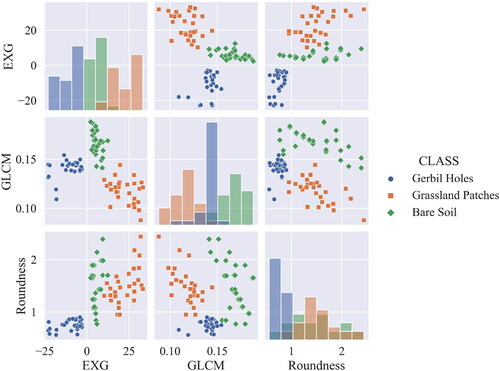
We created a scatter plot of the optimal feature subset to avoid subjectivity and randomness in feature threshold prediction, as shown in Figure 7. From the scatter plot, we found that the spectral characteristics of the three ground objects are highly different. Grassland patches had the highest EXG value, exceeding 5, while soil patches had an EXG value in the 0–10 range. Gerbil holes had the lowest EXG value, less than 0. In terms of texture characteristics, the GLCM of most grassland patches was higher than that of grassland and bare soil, reaching 0.150. The GLCM of gerbil holes was in the 0.120–0.150 range, while soil patches had the lowest GLCM characteristic of less than 0.120. The roundness of gerbil holes was lower than that of grassland and bare soil. Grassland and bare soil had a heavy overlap in this feature. As our main task was identifying gerbil holes, the shape remained a candidate feature value. The next step was to fine-tune the feature threshold based on prediction to obtain the rule set for UAV image classification.

Figure 7. Scatter plot of the distribution between optimal feature subset.

Based on the top-down classification rule, we used the minimum value as the extraction threshold of grassland after summarizing the EXG of all vegetation objects. After repeated adjustments on the training set, some bare soil was misclassified as grassland when the EXG threshold was less than 5, whereas some grassland could not be identified when it was greater than 5. Therefore, we achieved an optimized EXG threshold of 5, which effectively distinguished non-vegetation and vegetation. We then summarized the EXG of effective gerbil holes and found that the threshold value of the EXG rule had a remarkable difference in identifying the accuracy of gerbil holes. After several attempts, we were able to largely separate effective gerbil holes from the background (bare soil) when the EXG threshold was set to − 5. However, other bare soils were also classified as targets, as most of them had spectral characteristics similar to those of the effective gerbil holes (Figure 8(a)). The reason for this could be differences in the spectral characteristics of UAV imagery due to vegetation species. Therefore, we concluded that extracting effective gerbil holes via additional features was necessary.

Figure 8. Classification results of UAV imagery based on spectral features, texture features and geometric features.

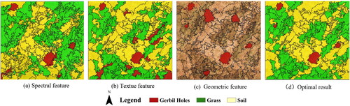
The GLCM is another critical feature that performs classification in desert grasslands. As shown in Figure 8(a), the process of UAV imagery classification still shows partial misclassification or leakage based on the EXG feature. Classifying ground objects further in desert grassland is necessary to improve accuracy and relies on texture features. The analysis of the UAV imagery properties indicates that the GLCM value of gerbil holes is in the range of 0.120–0.145, the GLCM value of grassland exceeds 0.151 and the GLCM value of bare soil is the lowest, less than 0.118. Therefore, non-vegetation objects can be separated from vegetation to a large extent by setting the GLCM to 0.151. In non-vegetation objects, effective gerbil holes can be extracted from the background by setting the GLCM in the range of 0.120–0.145. Figure 8(b) shows a spatial distribution of vegetation similar to the original image. However, we found that a minimal number of gerbil holes are still unidentified when the gerbil holes are extracted based on the texture feature. Some patches are mistakenly identified as gerbil holes. This phenomenon may be due to the overlapping of these patches with the texture characteristics of gerbil holes. Therefore, we need to identify gerbil holes further using shape features to eliminate such phenomena.

The effective gerbil holes are mostly subcircular, unlike the irregular shapes of most of the grassland and bare soil patches. This finding is consistent with the scatter plot analysis. The roundness property describes how similar an image object is to an ellipse, with a value equal to the radius of the largest closed ellipse minus the radius of the smallest closed ellipse. The closer an image object’s shape is to an ellipsoid, the lower its circularity is. Effective gerbil holes can be extracted from UAV images using the roundness feature. However, distinguishing patches consisting of grassland and bare soil is difficult. While the main task of the study is to identify effective gerbil holes, the calculation of vegetation cover is not the primary focus. Nevertheless, roundness can still be used for gerbil hole identification, with iterative testing performed on the training set all effective gerbil holes can be extracted when the roundness feature is less than 0.9. A minimal number of patches with shapes similar to mouse holes were also extracted (Figure 8(c)).

The classification accuracy was gradually improved through different segmentation parameters, layer superposition and optimization splicing of classification rules. The final classification result is shown in Figure 8(d), with all recommended segmentation parameters and classification thresholds detailed in Table 4.

Table 4. Recommended parameters for identifying effective gerbil holes in OBIA.

	Parameters or features	Values or threshold
Segmentation parameters in multiresolution segmentation	Scale parameter	170
	Shape factor	0.2
	Compactness value	0.3
Classification feature in OBIA	Spectral feature (EXG)	–5
	Texture feature (GLCM)	0.120–0.145
	Geometric feature (Roundness)	0.9

3.3. Maximum likelihood classification result

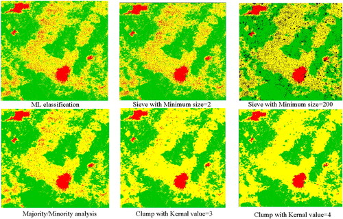
The ML classification results (Figure 9(a)) exhibit a large number of small spots, indicating the need for post-classification methods to improve the accuracy. Three methods were chosen for this purpose. First, spots smaller than 2 pixels were analyzed and sieved in Figure 9(b), but this had little effect on the classification results. In Figure 9(c), a minimum sieving size of 200 (the minimum area of gerbil hole patches) was used, which removed the noise on bare soil but also produced unclassified pixel spots. The majority/minority method was used in Figure 9(d), where the category of the central pixel was replaced by the category of majority/minority pixels in a kernel of size 3. This method removed some small spots. In Figure 9(e), the clump process was used, which used erosion and dilation to merge small patches. With a kernel value of 3, the majority of small spots could be merged into the background. However, increasing the kernel value to 4 in Figrue 9(f) resulted in a smoother image but also fragmented the effective gerbil hole patches. After analyzing the results, we used the clump method with a kernel value of 3 to remove the small spots from the ML classification results.

Figure 9. Maximum likelihood classification result with post classification.

3.4. Accuracy assessment of the two classification methods

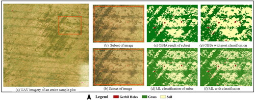
The two methods obtained similar grassland and soil patterns and could accurately locate the effective gerbil holes (Figure 10(c,d)). The small patch removal and fusion growth in the object-based method further improved the classification accuracy (Figure 10(e)). The grassland area produced by the rule-based method was smaller than that produced by ML, while the soil area was larger. ML measures the probability that a pixel belongs to a category and assigns the pixel to the most likely category, thereby easily disregarding the integrity of ground objects and inevitably resulting in fragmentation. The post classification- processing can effectively remove small spots in the classification results (Figure 10(f)).

Figure 10. UAV imagery and partly enlarged detail of classification results. (a) UAV imagery of an entire sample plot, (b) Subset of UAV imagery, (c) OBIA result of subset, (d) ML classification result of subset, (e) OBIA with post classification and (f) MLC with post classification

For further specific analysis, we formed a matrix for accuracy assessment based on the validation points generated from test samples. Accuracy indicators, including producer’s accuracy (PA), user’s accuracy (UA), kappa coefficients and overall accuracy (OA) for all three categories, were calculated. Additionally, the number of validation points was strictly controlled because their redundancy or inadequacy affects the evaluation accuracy (Pal and Foody et al. 2010). Tortora’s theory was used to determine the number of validation points (Tortora et al. 1978) using Eq. (8)(8) $$n=B(1-{\prod }_i)/{\prod }_i{b}_i^2$$(8) . (8) $$n=B(1-{\prod }_i)/{\prod }_i{b}_i^2$$(8) where $B$ is the upper $(\alpha /k)\times 100$ th percentile of the ${\chi }^2$ distribution with one degree of freedom. Let ${\mathrm{\Pi }}_i,$ $i=1,2,\dots ,k,$ be the proportion of the pixel in the category, and let $b_i={[B{\mathrm{\Pi }}_i(1-{\mathrm{\Pi }}_i)/n]}^{1/2}.$ There was no prior knowledge about the values of ${\mathrm{\Pi }}_i,$ and a ‘worst’ case calculation of sample size could be made assuming some ${\mathrm{\Pi }}_i=1/2$ and $b_i=b$ for all i.

Here, we required an absolute precision of $\pm 5\text{\%}$ for each proportion and a confidence coefficient of 95%. In the above equation, $b_i=0.05,i=1,2,3,$ and $\alpha =0.05.$ We obtained a random sample size of 2550 in the test data using ArcGIS10.5. The attribute class of each point was determined by visual interpretation to form a matrix for accuracy assessment. A total of 1241 of the 2550 validation points were in grassland, 1053 were in bare soil and 256 were in gerbil holes.

The final accuracy evaluation matrix is shown in Table 5. As a supervised classification, ML classification obtained an overall accuracy of 86.67% and a kappa coefficient of 0.77. Due to the integration of spectral, texture and geometric features, the overall accuracy of the object-based method reached 88.25%, which is 2.58% higher than that of ML. More importantly, the object-based method has a higher user accuracy than the ML method in identifying effective gerbil holes. The reason for this phenomenon may be because of the ‘salt and pepper’ noise generated by the ML method. Although clump classes were performed after classification, the high image resolution still showed a great amount of pepper noise in the results, reducing the classification accuracy.

Table 5. Accuracy assessments of two methods.

Classification method		Grassland	Gerbil hole	Bare soil	User’s accuracy (%)
OBIA	Grassland	1152	31	58	92.82
	Gerbil hole	24	209	23	81.64
	Bare soil	91	47	915	86.89
	Producer’s accuracy (%)	90.92	72.82	91.86
	Overall accuracy (%)	88.25	Kappa coefficients= 0.82
ML classification	Grassland	1012	67	162	81.54
	Gerbil hole	11	227	18	88.67
	Bare soil	31	51	971	92.21
	Producer’s accuracy (%)	96.01	65.79	84.36
	Overall accuracy (%)	86.67	Kappa coefficients = 0.77

Because the accuracy of the validation points method is likely to be unstable due to mixed objects (Ma et al. 2017a), the area-based accuracy assessment method was also performed in our research. We statistically analyzed the differences between the two classification methods in extracting the area of effective gerbil holes. The total number of effective gerbil holes for the test samples was 20, covering a total area of 725cm². The number of effective gerbil holes identified by rule sets was 17, achieving a recall rate of 85%. The covered area of the object-based method was 604 cm², with an accuracy of 83.31% in identifying the patch area. The number of effective gerbil holes identified by ML classification was 102, far exceeding the ground truth. However, the covered area of this method was only 570 cm², with an accuracy of 78.63% in identifying the patch area.

3.5. Relationship between effective gerbil holes and grass coverage

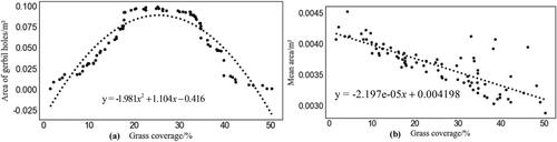
To examine the relationship between effective gerbil holes and grass coverage, we created a 5 × 4 grid using the fishnet tool in ArcGIS 10.5 (Figure 11(a)). The results showed a significant correlation between the area of effective gerbil holes and grass coverage. When grass coverage was less than 5%, there were few effective gerbil hole patches, which may be related to insufficient potential food resources. As grass coverage increased above 5%, the area of gerbil holes expanded with sparser grass coverage. The maximum area of effective gerbil holes was observed when grass coverage was in the range of 20–35%. However, as grass coverage continued to increase, the area of gerbil holes decreased, which may be because dense grasslands would undermine the escape ability of gerbils, increasing their risk of predation. Additionally, the mean area of gerbil hole patches decreased linearly with increasing grass coverage (Figure 11(b)). This phenomenon may be related to the increased grass cover, biomass and adequate food resources. In conclusion, the distribution of gerbil hole patches is influenced by grass coverage, and gerbils will only aggregate when the grassland is degraded to a certain degree.

Figure 11. Relationship between grass coverage and area of effective gerbil holes. (a) Area of gerbil holes and (b) Mean area.

4. Discussions

4.1. Efficient classification methods for UAV imagery

The supervised classification methods in OBIA are extremely labor-intensive and time-consuming, while the unsupervised classification methods are highly automated but have limited classification accuracy. In this article, an automatic method for the fast and accurate identification of effective gerbil holes in desert grasslands was proposed. Such approaches are crucial for carrying out near real-time rodent censuses. The key to this approach is defining the meaningful visual characteristics of effective gerbil holes. To overcome the image processing difficulties at high spatial resolution, we propose a data driven framework for parameter objectification rather than ‘trial and error’. We gathered UAV imagery from five sample plots and applied ESP2 and CFS to infer segmentation parameters and classification thresholds. Based on our analysis, we recommend the following rule sets: scale parameter of 107, shape factor of 0.2, compactness value of 0.3, EXG feature less than −5, GLCM value in the 0.120–0.145 range, and roundness feature value less than 0.9.

This study compared two methods for identifying effective gerbil holes. Both methods achieved high classification accuracy, exceeding 85%. However, the OBIA method had higher classification accuracy than ML, indicating that texture and geometric features can provide extra details and improve separability among objects. Furthermore, the OBIA method demonstrated better performance in recognizing the shape integrity of each gerbil hole patch. The OBIA method outperformed in extracting the number and area of effective gerbil holes, achieving 84.10% and 83.37%, respectively. When applied to the specific task of rodent censuses, the proposed system demonstrated that detecting gerbil holes in desert grassland is feasible when employing a simple RGB camera mounted on a UAV.

OBIA is a promising approach not only for supervised classification but also for unsupervised classification. The accuracy of the rule-based unsupervised classification method is facilitated by the application of ESP2 and CFS techniques. Despite iterative adjustments in optimizing segmentation parameters and selecting features, the above results show that homogeneous segmentation provides more available features that are crucial for extracting objects with specific shapes and distinct texture features. Conversely, feature selection reduces the dimension of features and improves the efficiency of object-oriented classification. Using this research as an example, the process of configuring features for every object during data labeling took over 12 min. After our parameter optimization, it only takes 1.7 min to classify a sample, which is an 86% improvement in efficiency. Considering that rule-based OBIA does not require manual sample selection, only a statistical analysis to determine segmentation parameters and thresholds is applied to a large amount of data from the same batch of flights. The labor and time costs spent on classification are much less than those of supervised classification methods.

4.2. Influences of grass coverage on M. unguiculatus

The number of effective gerbil holes is the most important indicator for densities of M. unguiculatus, and the patches formed by gerbils are an important parameter of grassland desertification. This article, for the first time, reported the effects of grass coverage on M. unguiculatus at a low-altitude remote sensing scale. The number of M. unguiculatus varied unimodally with grass coverage. When grass coverage increases or decreases from a certain threshold, the number of M. unguiculatus declines. This interaction reveals that when grassland degrades to a certain extent, the number of M. unguiculatus increases.

Previous studies have shown that rodent control alone has low efficiency in alleviating grassland degradation. The M. unguiculatus population can still recover after the cessation of rodent control (Tang et al. 2019). Increasing grass coverage may be a more feasible and ecologically sound pathway for controlling the M. unguiculatus population in practice.

5. Conclusion

Object-based image analysis offers a promising framework to address spectral mixing of different classes at subpixel scales. Previous studies have revealed the improvement in classification accuracy with object-based compared to pixel-based methods up to 31%. However, these comparisons were mostly conducted based on supervised classification, which varied not only in data and methods but also in the quantity and quality of training samples. In this article, rule-based classification is compared with ML for the first time, and the results show that by incorporating specific features of the target class, the rule-based algorithm can achieve superior results compared to pixel-based supervised classification. Moreover, rule-based algorithm has the feature of unsupervised classification, which has wide application value for massive remote sensing data processing.

The ESP2 and CFS algorithms are critical for determining the universal rule set. ESP2 defines a series of meaningful segmentation scale parameters for the image. But it is important that these scale parameters not be straightforwardly linked to a certain object, which produces some trouble to find an appropriate value of scale parameter without performing some attempts. In the future research, we will try scale parameter estimation which be linked to target object, based on labeled data. In this study, only three features were selected based on the CFS algorithm, which limited the extraction accuracy of effective mouse holes. The number of features can be increased in future research to achieve a balance between image processing speed and classification accuracy

The effectiveness of the rule-based classification method in extracting effective gerbil holes is affected by the timing of data acquisition and image resolution. During the spring when vegetation cover is low, gerbil hole patches are easily identified from UAV imagery. As vegetation coverage increases, occlusion and shadows in images become more prevalent, and the applicability of this method may be reduced. Our future studies will explore ways to better utilize multi-temporal data to improve segmentation and enhance the accuracy of effective gerbil hole identification. By incorporating texture and geometric features in the extraction of gerbil hole patches, the accuracy of this method is highly dependent on the ground sampling distance (GSD). Increasing the altitude of the UAV flight can improve the efficiency of image acquisition but may reduce image resolution and classification accuracy. Moreover, the thresholds of spectral features in the rule set may need to be adjusted when the UAV flight altitude changes. Further research is needed to validate these findings.

Disclosure statement

No potential conflict of interest was reported by the author.

Data availability statement

The data that support this study was shared on ScienceDB (scidb.cn).

Additional information

Funding

This work has been funded by the National Natural Science Foundation of China (NSFC) under grant Nos. 518650474 and 61806103. We would like to thank the anonymous reviewers for their helpful remarks.

References

- Addink EA, De Jong SM, Pebesma EJ. 2007. The importance of scale in object-based mapping of vegetation parameters with hyperspectral imagery. Photogramm Eng Remote Sens. 73(8):905–912.
- Belgiu M, Drǎguţ L. 2014. Comparing supervised and unsupervised multiresolution segmentation approaches for extracting buildings from very high resolution imagery. ISPRS J Photogramm Remote Sens. 96(Oct):67–75.
- Benz UC, Hofmann P, Willhauck G, Lingenfelder I, Heynen M. 2004. Multiresolution, object-oriented fuzzy analysis of remote sensing data for GIS-ready information. ISPRS J Photogrammetry Remote Sens. 58(3–4):239–258.
- Bhardwaj A, Sam L, Martín-Torres FJ, Kumar, R Akanksha. 2016. UAVs as remote sensing platform in glaciology: present applications and future prospects. Remote Sens Environ. 175:196–204.
- Blaschke T. 2010. Object based image analysis for remote sensing. ISPRS J Photogramm Remote Sens. 65(1):2–16.
- Charoenjit K, Zuddas P, Allemand P, Pattanakiat S, Pachana K. 2015. Estimation of biomass and carbon stock in Para rubber plantations using object-based classification from Thaichote satellite data in Eastern Thailand. J Appl Remote Sens. 9(1):096072.
- Chen G, Weng Q. 2018. Special issue: remote sensing of our changing landscapes with geographic object-based image analysis (GEOBIA). GISci Remote Sens. 55(2):155–158.
- Chen G, Weng Q, Hay GJ, He Y. 2018. Geographic Object-based Image Analysis (GEOBIA): emerging trends and future opportunities. Remote Sens. 55(2):159–182.
- Chen J, Yi S, Qin Y. 2017. The contribution of plateau pika disturbance and erosion on patchy alpine grassland bare soil on the Qinghai-Tibetan Plateau: implications for grassland restoration. Geoderma. 297:1–9.
- Costa H, Carrão H, Bação F, Caetano M. 2014. Combining per-pixel and object-based classifications for mapping land cover over large areas. Int J Remote Sens. 35(2):738–753.
- Dandois JP, Ellis EC. 2013. High spatial resolution three-dimensional mapping of vegetation spectral dynamics using computer vision. Remote Sens Environ. 136(5):259–276.
- Davis S, Trapman P, Leirs H, Begon M, Heesterbeek J. 2008. The abundance threshold for plague as a critical percolation phenomenon. Nature. 454(7204):634–637.
- Drăguţ L, Csillik O, Eisank C, Tiede D. 2014. Automated parameterisation for multi-scale image segmentation on multiple layers. ISPRS J Photogramm Remote Sens. 88(100):119–127.
- Drăguţ L, Tiede D, Levick SR. 2010. ESP: a tool to estimate scale parameter for multiresolution image segmentation of remotely sensed data. Int J Geogr Inf Sci. 24(6):859–871.
- Dronova I. 2015. Object-based image analysis in wetland research: a review. Remote Sens. 7(5):6380–6413.
- Eads DA, Biggins DE, Lei X, Liu Q. 2016. Plague cycles in two rodent species from China: dry years might provide context for epizootics in wet years. Ecosphere. 7(10):10–18.
- Espindola GM, Camara G, Reis IA, Bins LS, Monteiro AM. 2006. Parameter selection for region-growing image segmentation algorithms using spatial auto correlation. Int. J. Remote Sens. 27(14):3035–3040.
- Feng Y, Fan M, Gao Y, Li J, Zhang D, Wang S, Wang W. 2020. Epidemiological features of four human plague cases in the Inner Mongolia Autonomous Region China in 2019. Biosaf Health. 2(1):44–48.
- Guo R, Guan X, Zhang Y. 2015. Main advances in desertification research in China. J Arid Meteorol. 33(03):505–513.
- Guo Z, Huang N, Dong Z, Pelt RSV, Zobeck TM. 2014. Wind erosion induced soil degradation in northern China: status, measures and perspective. Sustainability. 6(12):8951–8966.
- Hall, M A, 2000. Correlation-Based Feature Selection for Machine Learning, The University of Waikato.
- Hall MA, Holmes G. 2003. Benchmarking attribute selection techniques for discrete class data mining. IEEE Trans Knowl Data Eng. 15(6):1437–1447.
- He Y,Huang X,Hou X,Feng Q. 2013. Monitoring grassland rodents with 3s technologies. Acta Pratacult Sin. 22(03):33–40.
- Ho TV, Rao PJ. 2016. Feature selection methods for object-based classification of tropical forest using spot 5 imagery. J Remote Sens GIS. 7(2):41–49.
- Jing L, Cheng Q. 2012. An image fusion method based on object-oriented classification. Remote Sens. 33(8):2434–2450.
- Johnson B, Xie Z. 2011. Unsupervised image segmentation evaluation and refinement using a multi-scale approach. ISPRS J. Photogramm. Remote Sens. 66(4):473–483.
- Juan S, Adam W, Felipe G. 2017. Towards the automatic detection of pre-existing termite mounds through UAS and hyperspectral imagery. Sensors. 17(10):1–15.
- Kang W, Liu S. 2014. A review of remote sensing monitoring and quantitative assessment of aeolian desertification. J Desert Res. 34(05):1222–1229.
- Laliberte AS, Browning DM, Rango A. 2012. A comparison of three feature selection methods for object-based classification of sub-decimeter resolution ultracam-l imagery. Int J Appl Earth Obs Geoinf. 15(4):70–78.
- Laliberte AS, Koppa J, Fredrickson EL, Rango A. 2006. Comparison of nearest neighbor and rule-based decision tree classification in an object-oriented environment. IEEE international Symposium on Geoscience & Remote Sensing. 3923–3926.
- Langner A, Hirata Y, Saito H, Sokh H, Leng C, Pak C, Raši R. 2014. Spectral normalization of SPOT 4 data to adjust for changing leaf phenology within seasonal forests in Cambodia. Remote Sens Environ. 143:122–130.
- Liu T,Ren H. 2022. Object-oriented extraction of paddy rice planting areas using phenological features from the GEE platform. J Agric Eng. 38(12):189–196.
- Liu J, Zhang J, Shijie L, Wang Z, Han G. 2019. Response of interspecific relationships among main plant species to the change of precipitation years in desert steppe. Acta Botanica Boreali-Occidentalia Sinica. 30(07):1289–1297.
- Liu Y, Fan J, Harris W, Shao Q, Zhou Y, Wang N, Li Y. 2013. Effects of plateau pika (Ochotona curzoniae) on net ecosystem carbon exchange of grassland in the three rivers headwaters region, Qinghai-Tibet, China. Plant Soil. 366(1–2):491–504.
- Lu D, Li G, Moran E, Kuang W. 2014. A comparative analysis of approaches for successional vegetation classification in the brazilian amazon. GISci Remote Sens. 51(6):695–709.
- Lü L, Wang R, Liu H, Yin J, Xiao J, Wang Z, Zhao Y, Yu G, Han X, Jiang Y. 2016. Effect of soil coarseness on soil base cations and available micronutrients in a semi-arid sandy grassland. Solid Earth Discuss. 7(2):549–556.
- Luo M, Wang Y, Xie Y, Zhou L, Qiao J, Qiu S, Sun Y. 2021. Combination of feature selection and catboost for prediction: the first application to the estimation of aboveground biomass. Forests. 12(2):216.
- Ma L, Cheng L, Han W, Zhong L, Li M. 2014. Cultivated land information extraction from high-resolution unmanned aerial vehicle imagery data. Appl Remote Sens. 8:1–25.
- Ma L, Cheng L, Li M, Liu Y, Ma X. 2015. Training set size, scale, and features in geographic object-based image analysis of very high resolution unmanned aerial vehicle imagery. ISPRS J Photogramm. Remote Sens. 102:14–27.
- Ma L, Fu T, Blaschke T, Li M, Tiede D, Zhou Z, Ma X, Chen D. 2017a. Evaluation of feature selection methods for object-based land cover mapping of unmanned aerial vehicle imagery using random forest and support vector machine classifiers. IJGI. 6(2):51.
- Ma L, Li M, Ma X, Cheng L, Du P, Liu YA. 2017b. Review of supervised object-based land-cover image classification. ISPRS J Photogramm Remote Sens. 130(Aug):277–293.
- Ma L, Yang Z, Zhou L, Lu H, Yin G. 2021. Local climate zones mapping using object-based image analysis and validation of its effectiveness through urban surface temperature analysis in China. Build Environ. 206:108348.
- Mallinis G, Koutsias N, Tsakiri-Strati M, Karteris M. 2008. Object-based classification using Quickbird imagery for delineating forest vegetation polygons in a Mediterranean test site. ISPRS J Photogramm Remote Sens. 63(2):237–250.
- Marmanis D, Wegner JD, Galliani S, Schindler K, Datcu M, Stilla U. 2016. Semantic segmentation of aerial images with an ensemble of CNNs. ISPRS Ann Photogramm Remote Sens Spatial Inf Sci. III-3:473–480.
- Meinel G, Neubert M. 2004. A comparison of segmentation programs for high resolution remote sensing data. Proceedings of 20th ISPRS Congress. Istanbul.
- Mengmeng D, Noboru N. 2017. Monitoring of wheat growth status and mapping of wheat yield’s within-field spatial variations using color images acquired from UAV-camera system. Remote Sens. 9(3):289–303.
- Pal M, Foody GM. 2010. Feature selection for classification of hyperspectral data by SVM. IEEE Trans Geosci Remote Sens. 48(5):2297–2307.
- Pang X, Guo Z. 2017. Plateau pika disturbances alter plant productivity and soil nutrients in alpine meadows of the Qinghai-Tibetan Plateau, China. Rangel J. 39(2):133–144.
- Pi W, Du J, Bi Y, Gao X, Zhu X. 2021. 3D-CNN based UAV hyperspectral imagery for grassland degradation indicator ground object classification research - ScienceDirect. Ecol Inf. 62:101278.
- Ran J, Lei D, Wen-Ji Z, Zhao-Ning G. 2016. Object-oriented aquatic vegetation extracting approach based on visible vegetation indices. Ying Yong Sheng Tai Xue Bao. 27(5):1427–1436.
- Rey N, Volpi M, Joost S, Tuia D. 2017. Detecting animals in African savanna with UAVs and the crowds. Remote Sens Environ. 200(2017):341–351.
- Richards JA, Jia XP, Richards JA. 2006. Remote sensing digital image analysis. Berlin Heidelberg: Springer.
- Shi X, Xue B. 2017. Parallelizing maximum likelihood classification on computer cluster and graphics processing unit for supervised image classification. Int J Digital Earth. 10(7):737–748.
- Sun Y, Ni Y, Chen J, Zheng J. 2018. Application of uav low-altitude image on rathole monitoring of eolagurus luteus. China Plant Prot. 39(04):35–43.
- Sun Y, Zhou Y, Yuan MS, Li WP, Luo YQ. 2018. UAV real-time monitoring for forest pest based on deep learning. Trans Chin Soc Agric Eng. 2018, 34(21):74–81.
- Tang Z, Zhang Y, Cong N, Wimberly M, Wang L, Huang K, Li J, Zu J, Zhu Y, Chen N. 2019. Spatial pattern of pika holes and their effects on vegetation coverage on the Tibetan plateau: an analysis using unmanned aerial vehicle imagery. Ecol Indic. (107):105551.
- Tehrany MS, Pradhan B, Jebuv MN. 2014. A comparative assessment between object and pixel-based classification approaches for land 5 imagery. Geocarto Int. 29(4):351–369.
- Tian Z,Fu Y,Liu S. 2013. Rapid crops classification based on UAV low-altitude remote sensing. Trans Chin Soc Agric Eng. 29(7):109–116.
- Tiede D, Hoffmann C. 2006. Process oriented object-based algorithms for single tree detection using laser scanning. International workshop:3D Remote Sensing in Forestry. Vienna; p. 162–167.
- Toomey M, Friedl MA, Frolking S, Hufkens K, Klosterman S, Sonnentag O, Baldocchi DD, Bernacchi CJ, Biraud SC, Bohrer G, et al. 2015. Greenness indices from digital cameras predict the timing and seasonal dynamics of canopy-scale photosynthesis. Ecol Appl. 25(1):99–115.
- Tortora R. 1978. A note on sample size estimation for multinomial populations. Am Stat. 32:100–102.
- Van Cleemput E,Vanierschot L,Fernández-Castilla B,Honnay O,Somers B. 2018. The functional characterization of grass- and shrubland ecosystems using hyperspectral remote sensing: trends, accuracy and moderating variables. Remote Sens. Environ. 209:747–763. 10.1016/j.rse.2018.02.030.
- Wei W, Fang J. 2009. Soil respiration and human effects on global grasslands. Global Planet Change. 67(1–2):20–28.
- Weissensteiner MH, Poelstra JW, Wolf JBW. 2015. Low-budget ready-to-fly unmanned aerial vehicles: an effective tool for evaluating the nesting status of canopy-breeding bird species. J Avian Biol. 46(4):425–430.
- Woodcock CE, Strahler AH. 1987. The factor of scale in remote sensing. Remote Sens Environ. 21(3):311–332.
- Wu XM, Liang CJ, Zhang DB, Yu LH. 2020. Identification method of plastic film residue based on UAV remote sensing images. Trans Chin Soc Agric Eng. 51(8):1–9.
- Yang CH, Everitt JH, Murden D. 2011. Evaluating high resolution SPOT 5 satellite imagery for crop identification. Comput Electron Agric. 75(2):347–354.
- Zhang X, Feng X, Jiang H. 2010. Object-oriented method for urban vegetation mapping using IKONOS imagery. Int J Remote Sens. 31(1):177–196.
- Zhou S, Han LL. 2021. A study of rodent monitoring in Ruoergai Grassland based on convolutional neural network. J Grass Forage Sci. (02):15–25.
- Zhu J, Yao J, Yu Q, He W, Xu C, Qin G, Zhu Q, Fan D, Zhu H. 2020. A fast and automatic method for leaf vein network extraction and vein density measurement based on object-oriented classification. Front Plant Sci. 11(5):1–15.