Simulation of visible light at night from infrared measurements using deep learning technique

Abstract

Improving visible imagery of clouds, especially at night, is of great importance for weather forecasting and warning. This study considered full-disc data obtained by the FengYun-4B satellite with the Advanced Geostationary Radiation Imager (AGRI) as an example, and adopted a deep neural network model to simulate the full-disc visible image using observed dynamic infrared data and surface background data to compensate for missing visible image data at night. The generated daytime visible image had the same characteristics as a corresponding GeoColor image, with an R² value of 0.99. The simulated night-time visible light, especially in the visualization of low cloud, clearly displayed and highlighted the characteristics of low cloud and fog, and could play an important role in application to near real-time weather forecasting at night. The simulation method could also be applied to the FY-3D/MERSI and Himawari-9/AHI satellite systems and to other infrared bands, similar to the FY-4B/AGRI system.

Keywords:

• Agri
• visible band
• infrared band
• DNN

1. Introduction

The FengYun-4B (FY-4B) satellite was successfully launched on 3 June 2021, and it is the first operational satellite of China’s second generation of geostationary orbit meteorological satellites (Yang et al. 2017; Lu et al. 2022). The FY-4B payload includes the Advanced Geostationary Radiation Imager (AGRI), which provides observational data in six visible and near-infrared bands and nine infrared bands with spatial resolution of 0.5–4.0 km, and temporal resolution of 15 min for overall coverage and 5 min for coverage of China (Xie et al. 2023). In comparison with the FY-4A/AGRI system, the FY-4B/AGRI system adds a low water vapor detection band (Zhu et al. 2023), and the spectral coverage of certain bands is adjusted to improve the observed signal (Li et al. 2022). FY-4B has new capabilities to capture aerosols and snow cover, to clearly distinguish between different stages of cloud, and to map upper- and mid-level atmospheric moisture.

Imager measurements of the FY-4 series, GOES-R series, Himawari-8/-9 and other new-generation geostationary satellites have been used in weather monitoring and forecasting, environmental monitoring and climate applications (Zhang et al. 2016). Typically, an imager operates in multiple spectral bands, covering the visible light, near-infrared and infrared regions. In addition to various quantitative products (Min et al. 2017), the image products of advanced imagers onboard geostationary satellites include brightness and temperature images, true colour composite images, fog, dust, severe convective storms and convective formation. True colour multiband composite images acquired in daytime are used in various applications such as monitoring weather and environmental changes. True colour images play an important role in weather and environmental monitoring because they can effectively reflect the surface characteristics, textural characteristics of high and low clouds and evolution of convective storm systems, especially the distribution and evolution of clouds in tropical cyclones. In application of an animation of cloud imagery obtained by an imager onboard a geostationary satellite, only visible band images can be used in daytime, while infrared band images are used at night. Consequently, there are inconsistencies in the continuity of observation targets and manifestation of visual artefacts between the day and night images, which cause difficulties in target recognition and thus impact monitoring applications.

The specific emissivity of cloud, fog and the surface under a clear sky differs between the middle-wave infrared and the thermal infrared regions. Fog is usually identified by the brightness temperature difference between the thermal infrared band and the middle-wave infrared band (Ma et al. 2022). The characteristics of cloud top height and cloud pressure can be effectively reflected by data in the thermal infrared bands. Those physical characteristics of clouds/fog in infrared bands enable simulation of visible band cloud images from infrared band measurements.

Previous studies have investigated the inversion of visible light images at night using night-time infrared channel images to overcome the problem of missing visible light images at night. For example, Kim et al. (2019) used Conditional Generation Adversarial networks (CGANs) to invert visible light images at night. Harder et al. (2020) used K-nearest neighbour regression, UNet, Unet ++ and a CGAN to invert visible light images at night. Cheng et al. (2022) used a CGAN to invert FY-4A/AGRI infrared channel images into night-time visible images and added cloud cover, wind speed, vortex, temperature and other information from ERA5 into the CGAN as model input. The models used in the above studies were trained using regional data and thus the inversion results were all regional images. The inversion of visible images of the entire disc at night has not previously been studied. The main difference between a full-disc image and a regional image is that areas affected by night or flare exist in the full-disc image, and the data of such areas cannot be used to train the model. If UNet, Unet ++, and CGANs are used to invert a visible image of the full-disc at night using an image as the input unit, impurities and flare will appear. Therefore, the above method is not applicable to the inversion of a visible image of the entire disc at night. However, using a regression network, such as a deep neural network (DNN), to eliminate the night and flare components of the training data through consideration of time zone and flare angle, and then integrating the remaining pixels together and training the model in pixel units, can overcome this problem, and a visible image of the entire disc can be reproduced.

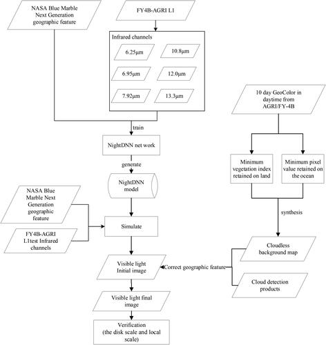
To invert a full-disc visible image at night, this study proposed a NightDNN based on the FY-4B/AGRI full-disc infrared channel and with reference to a DNN: (1) The NightDNN was used to simulate the FY-4B/AGRI visible image. (2) The input of the NightDNN included cloud-free true colour images as geographic information, which supported correction of geographical features in the simulation results. (3) The simulation of visible light was verified against parts of the image and the full disc.

2. Data and methodologies

On the basis of infrared band data from the FY-4B/AGRI system, this study developed a NightDNN to simulate visible images at night. First, the NightDNN was established using six infrared channels. Second, the training data set was established using data from 20220725 to 20220818, and the model was obtained after training. Third, the visible image was obtained via model calculation. A flow chart of the technical method is shown in Figure 1.

Figure 1. Flow chart of the methodology and technical approach.

2.1. Data preparation

The infrared channel data used in this study comprised FY-4B/AGRI 4-km resolution data provided by the National Satellite Meteorological Center. Data acquired at 02:00, 03:00, 04:00, 05:00, 06:00 and 07:00 UTC during 20220725–20220818 were used as the training set and the verification set to train the model using the NightDNN, and all data acquired on 20220905 and 20220906 were used as the test set to verify the performance of the model. Specific information regarding the data is listed in Table 1.

Table 1. FY-4B/AGRI L1B data information.

Satellite	Payload	Data	Role	Period
FY-4B	AGRI	L1	For obtaining infrared band data (Channel 7–15).	20220725–20220818,0905,0906
FY-4B	AGRI	L1 GEO	Geographic information data, including flare Angle information, for removing flares.	20220725–20220818,0905,0906
FY-4B	AGRI	GeoColor	True colour cloud image, used as a label for training models.	20220725–20220818,0905,0906
FY-4B	AGRI	CloudDetect	Cloud detection data, which is used to obtain longitude and latitude information of cloud-free points and non-cloud points in the reverse-performed night visible image are covered as pixels of the base image.	Same time as input data into the model
FY-4B	AGRI	LatLon	Latitude and longitude data.	–
FY-4B	AGRI	Land	For land/ocean labelling.	–

Processing of the training set and the verification set: The process involved acquisition of a surface feature image, data from infrared channels 7–15, and a GeoColor image of L1 data during 20220725–20220818. Concurrent flare angle information in the L1 GEO data was used to remove pixel points with a flare angle of <17 in the surface feature image, L1 infrared channel data, and GeoColor image (remove the flare). The latitude and longitude of each point in the surface feature image, L1 infrared channel data, and GeoColor image were obtained using LatLon data. The surface feature image, L1 infrared channel data, and points in the GeoColor image corresponding to the longitude range (Table 2) were retained according to the time of each data (excluding night). The remaining points of all the processed data (surface feature image, L1 infrared channel data (how to select the input infrared channel), and GeoColor image) were integrated into one-dimensional (1D) data, and 8192 (BatchSize) points were used as a batch to change the above 1D data into multiple batches of data. These batches of data were randomly assigned to the training set and the verification set in a ratio of 3:1. The surface feature image and the L1 infrared channel data comprised the model input of the training set and the verification set, while the GeoColor image represented the training label of the training set and the verification set (i.e. the target to be inverted by the model).

Table 2. Non-night partial longitude reservation range.

UTC	02:00	03:00	04:00	05:00	06:00	07:00
Upper limit of longitude	180°	140°	130°	80°	80°	80°
Lower limit of longitude	80°	20°	20°	20°	20°	20°

Processing of the test set: The test set was used to verify the performance of the model after model training. The L1 infrared channel data and a surface feature image at a certain time on 20220905 and 20220906 were resampled into 1D data for input into the model. Three 1D arrays were obtained by model inversion, which were then resampled into three two-dimensional (2D) images with the same length and width as those of the surface feature images and combined into a true colour map, i.e. the night-time visible light true colour map obtained by the NightDNN inversion.

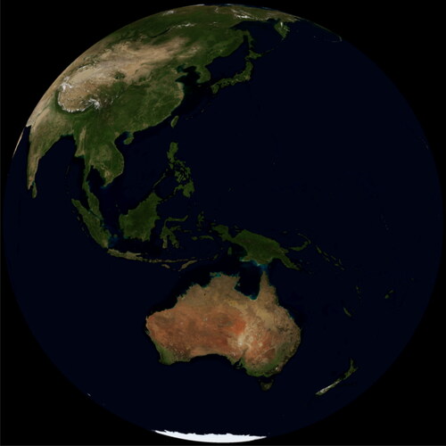
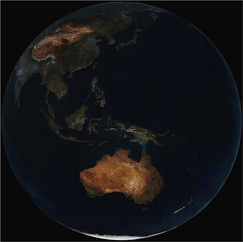
For simulation of the visible band data, eight images comprising 500-m-resolution surface feature data, acquired on 1–31 August 2004, were obtained from NASA’s Blue Marble Next Generation (https://visibleearth.nasa.gov/images/74117/ august-blue-marble-next-generation). The eight images were resampled to 4-km resolution and then synthesized. Finally, the synthesized images were projected onto the same latitude and longitude as the FY-4B/AGRI images. The latitude and longitude information of the FY-4B/AGRI image was obtained using FY-4B/AGRI LatLon data. The resultant surface feature image is shown in Figure 2.

Figure 2. Blue Marble Next Generation base map.

The map used for surface feature correction in the simulated visible band was the new cloud-free GeoColor image synthesized from 10-day FY-4B/AGRI images. FY-4B/AGRI GeoColor images with 1-km spatial resolution, acquired during daytime from 25 July 2022–2022 8 August 2022, were used for cloud-free synthetization.

Before simulation, the data of both the visible bands (x_r, x_g and x_b, representing the red, green and blue bands, respectively, for true colour image composition) and the infrared bands (C7, C8, C9, C10, C11, C12, C13, C14 and C15) need to be processed. The processing steps for the FY-4B/AGRI L1B data from 20220725 to 20220818 (02:00–06:00 UTC) and the corresponding true colour images were as follows. (1) Time zone processing: daytime visible bands for the true colour image were screened according to longitude and the processing method for the infrared bands was the same as that used for the visible bands. (2) Flare removal: points in the data where the solar flare angle was <17 were removed. (3) Conversion dimension: because all the data of each band are 2D and the simulation of the visible band requires 1D input data, the 2D data of each infrared band were converted (rearranged) to 1D data and filling values were removed. (4) Standardized processing: the values were normalized and distributed in the range of [−1, 1], and the peak value in the figure was taken as the median value of the final threshold range (near 0). In addition to the above processing, the L1B all-day data of FY-4B/AGRI on 20220905 and 20220906 (00:00–24:00 UTC) were subjected to anti-standardization processing; that is, the data after standardization were treated as the threshold range of the colour pictures [0–255].

2.2. Infrared channel selection

Clouds in visible light true colour images at night are mainly obtained through calculation and integration after features of infrared channel brightness and temperature data are extracted by the NightDNN. Therefore, selecting infrared channels with central wavelengths is particularly important. Specific parameters and main applications of all FY-4B AGRI bands are listed in Table 3. The infrared channel data of the L1 level data of FY-4B/AGRI were used in this study, among which AGRI has nine infrared channels (C7–C15).

Table 3. Specific parameters and main applications of all FY-4B AGRI bands.

Channel	Centre wavelength (μm)	Resolution (km)	Application
Channel1 (C 1, the same below)	0.47	1	Small particle aerosol, true colour synthesis
C 2	0.65	0.5	Vegetation, image navigation registration star observation
C 3	0.825	1	Vegetation, aerosols over water
C 4	1.379	2	Cirrus cloud
C 5	1.61	2	Low cloud/snow identification, water cloud/ice cloud identification
C 6	2.225	2	Cirrus, aerosol, particle size
C 7	3.75 (high)	2	High albedo targets
C 8	3.75 (low)	4	Low albedo target
C 9	6.25	4	Upper water vapor
C 10	6.95	4	Intermediate water vapor
C 11	7.92	4	Low-level water vapor
C 12	8.55	4	Total water vapor, cloud
C 13	10.8	4	Clouds, surface temperature, etc
C 14	12	4	Cloud, total water vapor, surface temperature
C 15	13.3	4	Clouds and water vapor

After conducting experiments, six of the channels (i.e. C9, C10, C11, C13, C14 and C15) listed in the table were selected as the infrared channel input of the NightDNN. Details of the experimental procedures and the results are presented in section 3.2.

2.3. Simulation of the visible band with the NightDNN

In this study, the NightDNN was proposed for simulation of visible band data. The land surface feature and cloud feature data were input into the DNN, and the FY-4B/AGRI true colour image was used as the label to train the network model for simulation of the visible band.

In a broad definition, a DNN contains three parts: an input layer, a hidden layer, and an output layer. The input layer is the first layer of the neural network, representing the original sample data input to the network. The output layer is the final layer of the neural network, which represents the final calculation results of the neural network. All neural network layers except the input and output layers belong to hidden layers. In a DNN, the number of neurons in the input layer is the number of features corresponding to the feature dimension of the input data (eg when the input is a picture, the data dimension is n*w*h*c, where n represents the number of pictures, w represents the width of the picture, h represents the height of the picture and c represents the number of channels of the picture (i.e. three for ordinary true colour images), and thus the number of neurons in the input layer is three). The data are input into the input layer, subjected to calculation using a certain formula for the input data feature dimension, and the output result represents the data available for the next layer. The calculation formula used in this study was the full link network layer, which can be expressed as follows: (1) $$A_i^{l+1}=w_{1i}^l\mathrm{*}{A}_1^l+w_{2i}^l\mathrm{*}{A}_2^l+\cdots +w_{ji}^l\mathrm{*}{A}_j^l+b_{ji}^l$$(1) where $A_i^{l+1}$ represents the i-th neuron of the neural network in layer l + 1, $A_j^l$ denotes the j-th neuron of the l-layer neural network, $w_{ji}^l$ represents the weights of the neural network in layer l from the j-th neuron to the i-th neuron and $b_{ji}^l$ denotes the amount of paranoia from the j-th neuron to the i-th neuron of the l-layer neural network.

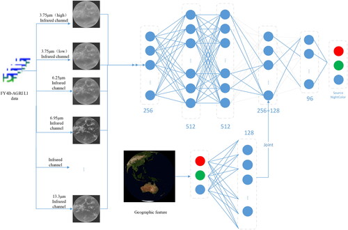
The NightDNN was developed to predict night-time visible band images. Because the night-time visible band has two different types of data (i.e. a colour background map and infrared band measurements), the NightDNN has two input layers corresponding to the two different types of inputs. The input layer of the infrared bands has four layers of full-link networks with 256, 512, 512 and 256 neurons, respectively, as the hidden layer. The input layer of the colour background image has a single layer of a full-link network with 128 neurons as the hidden layer. Finally, through a full-link network hidden layer of 96 neurons and the output layer of three neurons, the final output of three bands is obtained; the three bands represent the red, green and blue bands used for composition of the night-time true colour image. The topology of the NightDNN is illustrated in Figure 3.

Figure 3. NightDNN Network topology.

Training of the NightDNN was completed using a Tesla V100 SXM2 16 G GPU under a Linux operating system environment based on the Keras deep learning framework of Tensorflow. The NightDNN deep nerve was iterated 100 times, and the duration of each iteration was 10 min. To prevent overfitting of the NightDNN, further training was stopped when convergence of the MAE (mean absolute error) of the data set was verified. In this study, the MSE (mean square error) was used as the loss function in the training of the NightDNN model, and the MAE was used as an index for evaluation of the performance of the NightDNN. The formulas for calculation of the MSE and the MAE are shown as Eqs. (2)(2) $$\mathit{MSE}=\mathrm{ }\frac{1}{n}\sum _{i=1}^n{\left(\tilde{y}-y\right)}^2$$(2) and (3)(3) $$\mathit{MAE}=\mathrm{ }\frac{1}{n}\sum _{i=1}^n\left(|\tilde{y}-y|\right)$$(3) , respectively: (2) $$\mathit{MSE}=\mathrm{ }\frac{1}{n}\sum _{i=1}^n{\left(\tilde{y}-y\right)}^2$$(2) (3) $$\mathit{MAE}=\mathrm{ }\frac{1}{n}\sum _{i=1}^n\left(|\tilde{y}-y|\right)$$(3) where $\tilde{y}$ represents the NightDNN estimation results and $y$ represents the GeoColor true colour image pixels used to tag images.

2.4. Surface feature correction

Clouds in the night-time visible band will appear white owing to their low brightness temperature, and sometimes they can look similar to the white land because of the close brightness temperature between clouds and land, which might cause the model difficulty in distinguishing clouds from land. To resolve this problem, the AGRI cloud mask product is used to screen the cloud cover, which is used as supplemental information for predicting the visible bands and the corresponding true colour image composition.

In addition to using the cloud mask product, the 10-day cloud-free GeoColor image is used to replace the US base map because there is a large colour difference between the stationary US base map and near real-time dynamic FY-4B true colour image, which would need to be adjusted in the model. The BlueMarble base map is suitable as model input, however, it is different from the actual FY-4B/AGRI true colour map. For consistency in distinguishing between clouds and the background in the simulated true colour image at night, the FY-4B/AGRI synthetic background map with 4-km spatial resolution is used instead for cloud-free parts. The reason why the synthetic background map is not used initially in the visible light simulation is that the synthetic map would cause flaws in the simulation results.

The surface features are synthesized using multi-day GeoColor cloud images. Clouds and cloud shadows are removed to obtain cloud-free background data with only land and sea. The GeoColor cloud image was generated using multi-dimensional dynamic hybrid imaging technology (based on FY-4A/AGRI multi-dimensional dynamic hybrid imaging technology research). The technology used for cloud-free background data synthesis has been well verified using data from polar orbiting meteorological satellites with multiple synthesis standards (Qu et al. 2019). With the objective of cloud-free synthesis of imager data from geostationary meteorological satellites, the original method was improved in this study. The land part still uses the maximum vegetation index synthesis method (Qu et al. 2019). Because the vegetation index in a cloudy area is generally lower than that in a cloud-free area on land, the pixel value of the map where the vegetation index is higher is retained when the land part of the image is synthesized. The water part is then synthesized using the minimum method. Because the pixel value of cloud is higher than that of ocean, points with smaller pixel values are retained for the ocean part of the cloud-free background synthesis. In comparison with the FY-3D polar orbiting satellite, which only performs cloud-free synthesis for land, the FY-4B geostationary satellite adds clear-sky synthesis for water bodies, which produces images with coastlines, islands, water colours and river alluviations that have clear texture and are close to the real sea surface.

3. Result

3.1. NightDNN model training

Figure 4 shows graphs of the MAE of the NightDNN validation data set, validation data set loss and training data set loss for each training iteration. As the number of training iterations increased, the MAE and the loss curves decreased continuously, indicating gradual improvement in the learning ability of the NightDNN. With increase in the number of training iterations, the slope of the MAE curve gradually approached zero, indicating that the model converged to an optimum state and that the training could be stopped. To prevent overfitting of the NightDNN in the experiment, we adopted a learning rate stepwise linear decay training strategy with an initial learning rate of 1*e⁻⁵. Calculation of the stepwise linear attenuation was performed using Equation (4)(4) $$\widetilde{lr}=lr\mathrm{ }\times \mathrm{ }\frac{1}{(1+\mathrm{ }\mathit{decay}\mathrm{*}\mathit{epoch})}$$(4) : (4) $$\widetilde{lr}=lr\mathrm{ }\times \mathrm{ }\frac{1}{(1+\mathrm{ }\mathit{decay}\mathrm{*}\mathit{epoch})}$$(4) where $\widetilde{lr}$ represents the attenuation, $lr$ represents the attenuation vector, $\mathit{decay}$ represents the attenuation coefficient (set at 1*e⁻⁶) and $\mathit{epoch}$ represents the current number of iterations.

Figure 4. Loss and MAE curves during NightDNN training.

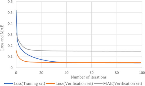
The loss function is the MSE, and therefore a gap exists between the loss and the MAE.

3.2. Visible band simulated by combinations of different infrared bands

The visible band simulation was performed using FY-4B/AGRI data from 20220725 to 20220818 (only data from 02:00–06:00 UTC were selected) as the training set and the validation set. The training and validation sets were randomly assigned in a 3:1 ratio. The full-day data from 20220905 to 20220906 were used as the test set. The true colour image data corresponding exactly to the times of the training set and the validation set were used as labels for training and validation.

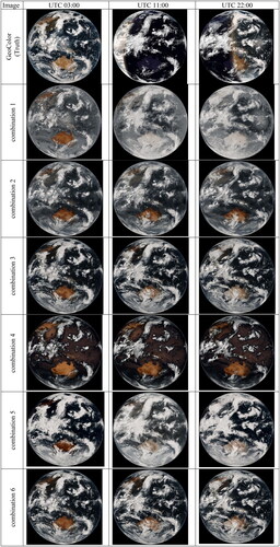
Figure 5 shows the visible band images simulated by different channel combinations of FY-4B/AGRI and the GeoColor visible band at 03:00, 11:00 and 22:00 UTC on 20220905 for comparison purposes, where x_r, x_g and x_b represent the red, green and blue bands, respectively, used for the colour image composition. The model using combination 1 (x_r + x_g + x_b + C7 + C8) as input clearly makes the cloud darker overall and diminishes the stereoscopic effect. At night, all the land is predicted to be cloud, and the prediction of flare in the picture is poor. With combination 2 (water vapor channel combination), the colour is slightly greyer in cloudless areas, and the clouds near the South Pole appear fog-like with no characteristic cloud features. With combination 3 (x_r + x_g + x_b + C13 + C14 + C15), there are no missing clouds, and the cloud types are broadly the same as those in the GeoColor image, but some cloudless land is predicted to be cloud at night. Combination 4 (x_r + x_g + x_b + C12) predicts a lot of missing cloud. Combination 5 (x_r + x_g + x_b + C12 + C13 + C14 + C15) predicts cloud with distorted colour, and the overall effect of the forecast map is not as satisfactory as that achieved when only C13, C14 and C15 are used (combination 3). Combination 6 (x_r + x_g + x_b + C9 + C10 + C11 + C13 + C14 + C15) involves the addition of C9, C10 and C11 based on C13 and C15. The stereoscopic effect of the clouds is enhanced, the colour is brighter, and the effect of the prediction map is better than that achieved when using only C13, C14 and C15. In summary, when the input data comprise combination of the colour base map, C9, C10, C11, C13, C14 and C15, the simulation effect is the best among all the combinations considered.

Figure 5. Comparison of FY-4B/AGRI GeoColor images and visible bands simulated with different infrared band combinations at three times on 20220905. (combination 1: x_r + x_g + x_b + C7 + C8; combination 2: x_r + x_g + x_b + C9 + C10 + C11; combination 3: x_r + x_g + x_b + C13 + C14 + C15; combination 4: x_r + x_g + x_b + C12；combination 5: x_r + x_g + x_b + C12 + C13 + C14 + C15; combination 6: x_r + x_g + x_b + C9 + C10 + C11 + C13 +C14 + C15).

3.3. Modification of surface features

Although the true colour image predicted by the model when using the colour base map from BlueMarble, together with C9, C10, C11, C13, C14 and C15 as input, is the best of all the combinations considered, there are still some cases where cloud-free land is predicted to be cloud. To resolve this problem, surface feature correction was performed on the predicted image using the AGRI cloud mask product (Min et al. 2017) as supplemental information, and non-cloud parts were replaced by the cloud-free background map from the synthesized 10-day FY-4B true colour images.

Figure 6 shows the synthesized cloud-free background image of FY-4B/AGRI true colour images from 20220715 to 20220818. Evidently, only clear background data are retained, and the vegetation texture, mountain texture, desert and Gobi texture on the surface, and snow-covered mountain data in plateau areas are well preserved. In terms of water bodies, the Yellow River and the Yangtze River estuary sediment, together with the water colour are effectively reflected. The pale blue reefs in Southeast Asia and Australia also remain. The overall effect of the clear-sky background data is considered realistic and suitable for input into the DNN.

Figure 6. Synthetic clear-sky background map data from FY-4B/AGRI as the background map.

3.4. Verification of visible band simulation

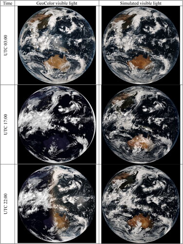
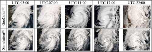
Three representative real images—full day, full night and alternation of day and night—were selected to verify the effect of simulation of the visible band. Figure 7 shows the observed true colour image and the simulated true colour image observed by the FY-4B/AGRI at 03:00, 15:00 and 22:00 UTC on 20220905. The visible cloud image produced by the model after adding the cloud mask as supplemental information is closest to the real image. The simulated visible band image can reproduce the real daytime visible band image reasonably well. In areas where the real visible band cannot be displayed, the simulation results create realistic visible band images and realize continuous observation of cloud features. At 03:00 UTC, the coverage of the FY-4B/AGRI is of full daytime data. At that time, the cloud patterns of the predicted image (right) and the real image (left) are broadly consistent and there are no obvious lost clouds. The flare in the left-hand image is no longer present in the right-hand image. In comparison with the real image on the left, the predicted image on the right has fewer scattered clouds (white scatter on the sea surface) because scattered clouds cannot be displayed in infrared bands. Additionally, the background colour of the predicted map is darker. This is because the real map is affected by sunlight that makes the background map brighter, while the background colour of the predicted map is provided by the quasi-static base map that is not affected by sunlight. The full night coverage visible band image simulated by the model is shown for 17:00 UTC. The clouds are clearly displayed in the predicted image. However, certain places in Australia that are not clouds are predicted to be clouds. This is because the model predicts clouds based on brightness temperatures and the brightness temperatures at night in some places are too low (eg close to the brightness temperatures of clouds), thereby causing misprediction. The predicted clouds have transversals, which are due to the presence of transversals in the brightness temperatures themself, and these transversals can be removed via de-transversal processing. The simulated FY-4B/AGRI true colour image of alternation between day and night is shown for 22:00 UTC. The cloud pattern is mostly correct, and all the clouds that were not visible at night have been restored, although some night-time low clouds have the same colour as different clouds in the predicted image.

Figure 7. Observed visible band and the simulated visible band of FY-4B/AGRI true colour images on 20220905 at 03:00, 17:00 and 22:00 UTC.

The local effect of the visible band was simulated and verified against four typical meteorological events and geographical images in the true colour image, i.e. the typhoon region, Southern Hemisphere region, low cloud region and flare region.

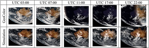
Figure 8 shows the FY-4B/AGRI-observed true colour images of the Southern Hemisphere region and the corresponding simulation at different times on 20220905. The simulated Southern Hemisphere cloud system clearly fits the real Southern Hemisphere cloud system very well. Visible observations in this area at night are lacking, but the simulation results effectively provide an accurate visible image of this area for continuous monitoring of cloud, land and ocean features.

Figure 8. Observed FY-4B/AGRI true colour images of Southern Hemisphere region and the corresponding simulated images at different times on 20220905.

The local effect of the simulated visible band is verified against two typical meteorological events and geographical images: the typhoon region and the Southern Hemisphere region where the cloud cover, land and sea elements are more obvious. Figure 9 shows the observed visible typhoon area of FY-4B/AGRI true colour images and the corresponding simulation at different times on 20220905. The typhoon was named as the eleventh typhoon of 2022, i.e. Typhoon Xuan Lanuo. The cloud characteristics and dynamics of Typhoon Xuanlano are well represented in the simulated image. The cloud distribution and the cloud texture are clear, and the process of transition from giant circulation to a gradually weakening cyclone is coherent and smooth. Thus, accurate simulation could help in monitoring the evolution process of typhoons and in analysis of their characteristics.

Figure 9. Observed FY-4B/AGRI true colour images and the corresponding simulated images of Typhoon Xuanlano at different times on 20220905: (a) GeoColor visible light images of typhoon area and (b) simulated visible light images of typhoon area.

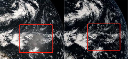
Figures 10 and 11 show the true colour image simulation results of the low cloud area and flare area, respectively, at 22:00 UTC (night) on 20220905. The fuzzy low clouds in the red box (left) become clear and layered in the corresponding simulation (right). In Figure 11, the visible flare present in the red box (left) is also lost in the simulated image (right). The above results show that the visible image generated by this method can clearly display and highlight the characteristics of low clouds and eliminate flare.

Figure 10. Medium–low clouds in (left) FY-4B/AGRI true colour image and (right) simulated low clouds on 20220905 at 22:00 UTC.

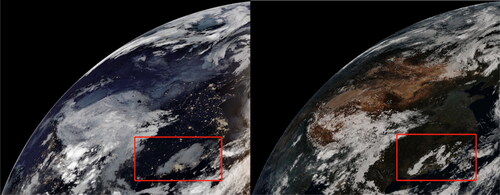
Figure 11. FY-4B/AGRI true colour image and the corresponding simulated image for flare at 22:00 UTC on 20220905.

Table 4 lists details of the fitting results of the visible light images simulated for 20220905 and 20220906 at 03:00, 04:00 and 07:00 UTC and the corresponding GeoColor visible light images. The RMSE values of 8.2–8.6 and the coefficient of determination (R²) values of up to 0.99 indicate that the simulated visible light images effectively reproduce the GeoColor visible light images.

Table 4. Fitting results of simulated visible light and corresponding GeoColor visible light.

UTC	0905/3:00	0905/4:00	0905/7:00	0906/3:00	0906/4:00	0906/7:00
RMSE	8.31	8.25	8.59	8.29	8.27	8.57
R^2	0.99	0.99	0.99	0.99	0.99	0.99

To understand the contribution factor of each band to the final simulation, Table 5 lists the average weights of all the input bands in the model. The weights of the red, green and blue bands in the background map are lower than those of the infrared band. This is because the background map is used as one input in the model for all times, i.e. it remains unchanged unlike the data of the infrared bands. The weight of the blue band in the base map is higher than that of the red and green bands. This is because the proportion of ocean in the base map is much higher than that of land, and because the colour of the ocean is mainly determined by the blue band. Corresponding to the six infrared bands, the role of the three water vapor absorption bands (i.e. C9, C10 and C11) in the model is mainly to improve the representation of convective clouds and typhoons, and for determination of cloud shape. The extraction of cloud features is mainly determined by the C13, C14 and C15 bands (the results of x_r + x_g + x_b + C13 + C14 + C15 are closer to the results of x_r + x_g + x_b + C9 + C10 + C11 + C13 + C14 + C15). Therefore, the weights of C13, C14 and C15 are higher than those of C9, C10 and C11.

Table 5. Weight of each input band in the model.

Satellite	Load	Channel	Weights
FY-4B	AGRI	x_r	0.269
FY-4B	AGRI	x_g	0.295
FY-4B	AGRI	x_b	0.344
FY-4B	AGRI	C9	0.370
FY-4B	AGRI	C10	0.376
FY-4B	AGRI	C11	0.375
FY-4B	AGRI	C13	0.473
FY-4B	AGRI	C14	0.470
FY-4B	AGRI	C15	0.548

4. Conclusion and discussion

This study proposed a visible light simulation algorithm based on deep learning for the FY-4B/AGRI. The method uses FY-4B/AGRI infrared channel data and input data to input geographical features and cloud features into a DNN to synthesize and generate a prediction of visible light at night, and it uses GeoColor to synthesize images to correct geographical features in the simulation results, and to finally obtain an image with reasonable simulation of visible light. In comparison with other existing methods, the approach proposed in this study has three innovations. First, the NightDNN no longer processes image to image, but pixel to pixel. To deal with flare and the night part of a full-disc image, pixels affected by flare and night are removed, and the 2D image is converted into 1D pixels as input data to simulate visible light. The output result of the model is no longer a night-time visible image, but the pixels of the image. The second innovation is the incorporation of geographic information into the model. Because of the lack of geographic information in the infrared channels, the proposed model incorporates a base map with geographic information. The third innovation involves experimentation with all the FY-4B/AGRI infrared channels and selection of the optimal combination as input for the model. The visible light simulation method proposed in this study can create realistic daytime and night-time visible light images and overcome the problems of lack of geographic information and lack of cloud features at night. The visible light images generated can be applied to the earth true colour map display, as well as the monitoring and analysis of complex weather events such as clouds, fog and typhoons during the day and at night. Specifically, it can provide details of night-time weather and provide data support for weather forecasting and meteorological research.

For cloud detection at night, different responses of infrared bands under the conditions of clouds and clear skies are usually used to distinguish cloud types and phases. Because cloud characteristics are mainly reflected by cloud phase state (including ice clouds, water clouds and mixed clouds, etc.) and cloud top parameters (including cloud top height, cloud top temperature, cloud top pressure, etc.), the phase and height information of clouds should be considered in the simulation of cloud in the visible band at night.

Cloud phase state and cloud top parameters are effectively reflected by measurements from infrared bands. Ice clouds and water clouds react differently to similar incident radiation. For example, ice clouds absorb more at 10 and 12 μm than water clouds with the same water content owing to difference in the refractive index. From 8–11 μm, changes in the microphysical characteristics of clouds can be detected. Additionally, owing to absorption by carbon dioxide, the transparency of the atmosphere decreases with increasing wavelength, and the radiation value of the band between 13.3 and 15 μm decreases. Therefore, MODIS also uses the CO₂ absorption zone near 15 μm for retrievals of cloud phase state and cloud top parameters (Levy et al. 2009). Six infrared bands ranging from 10.8 to 14.4 μm are used in the retrieval of MODIS cloud top parameters. For GOES-R, cloud top height is retrieved by the ABI cloud height algorithm using three bands: 11.2, 12.3 and 13.3 μm. The 7.4, 8.5, 11.2, 12.3 μm bands are used to retrieve cloud types and cloud phase states (Pavolonis 2010).

Changes in the atmosphere caused by water vapor are sometimes not visible in the infrared window bands, but the water vapor absorption bands can be affected substantially (Heidinger and Straka 2010). Krebs et al. (2007) used water vapor absorption bands to detect cirrus clouds in MeCiDA, a second-generation cirrus detection algorithm designed for Meteosat. In GOES-R cloud detection, Heidinger and Straka used either a 7.0 μm band or a 7.4 μm band (Heidinger and Straka 2010) to detect cirrus clouds.

Fog is formed by reduction in the near-surface temperature and the unsaturated condensation of water droplets or ice crystals in the air. It has strong grounding property, and the temperature of fog top is close to that of the surface (Ma et al. 2022). The specific emissivity of cloud and fog in the middle-wave infrared band (3.9 μm) is different to that of the surface under a clear sky. The specific emissivity of cloud and fog in this band is <1, while the approximate blackbody emissivity of the surface is equal to 1 (Ma et al. 2022). Therefore, low cloud and fog can be distinguished using the 3.75–3.9 μm band.

In this study, nine infrared bands of the FY-4B/AGRI were classified and freely combined and input into a DNN with geographical background correction for visible band simulation. For the best combination, the contributions of the red, green and blue bands in the background map are lower than those of the infrared bands owing to the fact that they represent a quasi-static input in comparison with the infrared bands. The contribution of the blue band in the background map is higher than that of the red and green bands because the proportion of ocean in the background map is much higher than that of land, and because the colour of the ocean is mainly determined by the blue band. For the corresponding six infrared bands, the function of the three water vapor absorption bands (i.e. C9, C10 and C11) in the model is mainly to improve the representation of convective clouds and typhoons. For cloud shape, the extraction of cloud features is mainly determined by the C13, C14 and C15 bands (the result of x_r + x_g + x_b + C13 + C14 + C15 is closer to that of x_r + x_g + x_b + C9 + C10 + C11 + C13+ C14 + C15). Additionally, South Pole clouds were fully predicted by the model only when C13, C14 and C15 were included.

Acknowledgments

The authors thank anonymous reviewers for their constructive comments to improve the quality of this paper.

Disclosure statement

No potential conflict of interest was reported by the author(s).

Data availability statement

The datasets available from the corresponding author on reasonable request.

Correction Statement

This article has been corrected with minor changes. These changes do not impact the academic content of the article.

Additional information

Funding

This research was funded by the National Natural Science Foundation of China, grant number 42201399.

References

- Cheng W, Li Q, Wang Z, Zhang W, Huang F. 2022. Creating synthetic night-time visible-light meteorological satellite images using the GAN method. Remote Sens Lett. 13(7):738–745. doi:10.1080/2150704X.2022.2079016.
- Harder P, Jones W, Lguensat R, Bouabid S, Fulton J, Quesada-Chacón D, Marcolongo A, Stefanovi S, Rao Y, Manshausen P, Watson-Parris D. 2020. NightVision: generating nighttime satellite imagery from infra-Red observations. Paper presented at: Virtual-only Conference. Tackling Climate Change with Machine Learning workshop at NeurIPS 2020; Dec 8. https://arxiv.org/abs/2011.07017
- Heidinger A, Straka WC. 2010. Algorithm theoretical basis document for ABI Cloud Mask. Maryland: NOAA NESDIS Center for Satellite Applications and Research; 1–86. https://www.star.nesdis.noaa.gov/star/contact.php
- Kim K, Kim JH, Moon YJ, Park E, Shin G, Kim T, Kim Y, Hong S. 2019. Nighttime reflectance generation in the visible band of satellites. Remote Sens. 11(18):2087. doi:10.3390/rs11182087.
- Krebs W, Mannstein H, Bugliaro L, Mayer B. 2007. A new day- and night-time meteosat second generation cirrus detection algorithm MeCidA. Atmos Chem Phys. 7(24):6145–6159. doi:10.5194/acp-7-6145-2007.
- Levy RC, Remer LA, Tanré́ D, Mattoo S, Kaufman YJ. 2009. Algorithm for remote sensing of tropospheric aerosol over dark targets from MODIS: Collections 005 and 051: revision 2. MODIS Algorithm Theoretical Basis Document. 1–96.
- Li J, Menzel WP, Schmit TJ, Schmetz J. 2022. Applications of geostationary hyperspectral infrared sounder observations: progress, challenges, and future perspectives. Bull Am Meteorol Soc. 103(12):E2733–E2755. doi:10.1175/BAMS-D-21-0328.1.
- Lu W, Qiu Y, Yang L, Huang Y. 2022. Analysis of the ranging systematic error of the FY-4 geostationary satellite and its influence on orbit determination. Chin J Sci Instrum. 43(2):73–83.
- Ma H, L Y, Wu X, Ran Y, Yan J. 2022. Automatic detection of night land fog based on H8/AHI satellite data. Remote Sens Technol Appl. 37(2):408–415.
- Min M, Wu C, Li C, Liu H, Xu N, Wu X, Chen L, Wang F, Sun F, Qin D, et al. 2017. Developing the science product algorithm testbed for Chinese next-generation geostationary meteorological satellites: fengyun-4 series. J Meteorol Res. 31(4):708–719. doi:10.1007/s13351-017-6161-z.
- Pavolonis M. 2010. GOES-R Advanced Baseline Imager (ABI) algorithm theoretical basis document for cloud type and cloud phase. Maryland: NOAA NESDIS Center for Satellite Applications and Research; 1–86. https://www.star.nesdis.noaa.gov/star/contact.php
- Qu J, Yan J, Wang Y. 2019. Global clear-sky data synthesis technology based on FY-3D MERSI-II instrument. Meteorol Sci Technol. 47(4):539–545.
- Xie L, Wu S, Wu R, Chen J, Xu Z, Cao L. 2023. Cross-comparison of radiation response characteristics between the FY-4B/AGRI and GK-2A/AMI in China. Remote Sens. 15(3):779. doi:10.3390/rs15030779.
- Yang J, Zhang Z, Wei C, Lu F, Guo Q. 2017. Introducing the new generation of Chinese geostationary weather satellites, Fengyun-4. Bull Am Meteorol Soc. 98(8):1637–1658. doi:10.1175/BAMS-D-16-0065.1.
- Zhang P, Guo Q, Chen B, Feng X. 2016. The Chinese next-generation geostationary meteorological satellite FY-4 compared with the Japanese Himawari-8/9 Satellites. Adv Meteorol Sci Technol. 6(1):72–75.
- Zhu Z, Shi C, Gu J. 2023. Characterization of bias in Fengyun-4B/AGRI infrared observations using RTTOV. Remote Sens. 15(5):1224. doi:10.3390/rs15051224.