A generalized framework for quantifying and monitoring the severity of meteorological drought

Abstract

The current study proposes a new framework for quantifying and monitoring the severity of meteorological drought. The proposed framework consists of three phases. The first phase of the framework uses K-component Gaussian Mixture Distribution (GMD) in the computation. The second phase is mainly based on the dissimilarity matrix-based clustering using C-index and Monte Carlo Feature-based Selection (MCFS) method. The third phase uses the Markov chain, transition probabilities and a non-homogeneous Poisson process under the Bayesian estimation. The Relative Importance (RI) values are used to choose appropriate stations. The Deviance Information Criteria (DIC) is used to check model suitability, and Root Mean Square Error (RMSE) is utilized for determining model performance. The proposed framework is validated to the 52 meteorological stations in Pakistan for 49 years from 1968 to 2016. Moreover, the outcomes of the current analysis provide insight to quantify and monitor meteorological drought comprehensively and accurately.

Keywords:

• Meteorological drought
• standardized precipitation evapotranspiration index
• k-component Gaussian mixture distributions
• hierarchical clustering
• Bayesian estimation

1. Introduction

Drought is the shortage of water reserves compared to normal conditions due to the high temperature and below-average precipitation in an area for a period (Moazzam et al. 2022; Shorachi et al. 2022) . It is one of the most destructive and complex natural disasters that may lead to severe health, social and agricultural losses (Kron et al. 2019). In addition, it adversely affects ecosystems, livelihoods, and socioeconomic, and environmental conditions (Asmall et al. 2021; Oyounalsoud et al. 2022). The drought effects include wildfire, food crisis, food shortages, immigration and irregulating in climate and hydrological cycle (Zeng et al. 2022). Drought is generally classified into four major types: meteorological drought, ie insufficient precipitation, agricultural drought, ie insufficient soil moisture; hydrological drought, ie groundwater & water flow reduction and socio-economic drought, ie the gap between water demand and supply (Zhang et al. 2020; Wang et al. 2021).

The meteorological drought is the leading type of drought that may occur due to a shortage of precipitation (Jiménez-Donaire et al. 2020). Due to the shortage of precipitation for a moderate period, meteorological drought propagates to agricultural drought, ie the agricultural land becomes soil moisture deficient, and the long duration of this situation shifts prominently toward hydrological drought (Shah et al. 2021). The water reservoirs are highly affected due to the hydrological drought, and the effect of water shortage remains for a long period (O’Connor et al. 2022). All these types of droughts are interconnected and occur sequentially, which may lead to some difficulties in distinguishing between these types and generate an uncertain decision in quantifying the drought effect. Drought events have various interconnected properties, ie recurrence interval, intensity, duration and severity. Drought is a complex natural hazard that cannot be eliminated, but its effect could be reduced or eliminated by utilizing decision support tools for quantifying the physical characteristics (duration, intensity and severity) of droughts (Anshuka et al. 2019; Orimoloye 2022). For this purpose, globally the researchers and climatologists utilized drought indicators or indices to analyse the meteorological and hydrological cycles and use this information to monitor the drought community for framing drought policies and making decisions (Alahacoon and Edirisinghe 2022; Kafy et al. 2023).

The subsequent decision support tools highly rely on indices and indicators, widely used to quantify the drought events along their intensities, severity and magnitude (Alahacoon and Amarnath 2022; Vélez-Nicolás et al. 2022). Drought indices are used in the broad sense to aggregate parameters, ie precipitation, temperature, humidity, streamflow, etc. and are formulated to monitor drought events with all their characteristics (Niaz et al. 2021a, 2021b, 2022d). Based on the influential hydroclimatic variables, drought indices estimate a single value which has a significant advantage over mere raw data in quantifying drought characteristics. With the passage of time, the drought assessment tools remain under significant progress and improvements. Drought indices have a highly significant role in drought assessment studies and the researchers developed various drought indices for studying different types of droughts at their multiple levels/conditions (Alahacoon and Amarnath 2022; Vélez-Nicolás et al. 2022). The Standardized Runoff Index (SRI) is applicable to assess and analyse the hydrological drought events and soil moisture percentile for agricultural drought assessment (Tigkas et al. 2016; Babre et al. 2022). Climatologists around the world utilized the Standardized precipitation index (SPI) proposed by McKee et al. (1993), the Standardized precipitation evapotranspiration index (SPEI) proposed by Vicente-Serrano et al. 2010 and the Standardized Precipitation Temperature Index (SPTI) purposed by Ali et al. (2017) for the assessment of meteorological, agricultural and hydrological drought event based on various time scale. Harisuseno (2020) used SPI, RAI (Rainfall Anomaly Index) integrated through SSI (standardized Stream flow Index) in a comparative study to assess the drought severity and duration in Pekalen River Basin, Indonesia. Ellahi et al. (2020) and Ellahi et al. (2021) utilized 6-month and 12-month SPI utilized for agricultural and hydrological drought assessment. Liu et al. (2021) utilized SPI and SPEI at multiple time scales in the spatiotemporal analysis of drought in Sichuan Province, China. Sein et al. (2021) used SPEI at a 3-month time scale for the assessment of agricultural drought to analyse the spatial-temporal pattern of drought and its effect on crop production in Myanmar. In contrast, the SPI is widely used as a drought monitoring tool but has some limitations (Mishra et al. 2022; Niaz et al. 2022a, 2022b, 2022c). The index only relies on precipitation and does not consider other variables influencing drought severity, such as temperature, evapotranspiration, etc. Moreover, the areas where the evapotranspiration is high and low precipitation, or the precipitation is highly variable SPI may underestimate drought severity (Dibi-Anoh et al. 2023). Meanwhile, SPI may overestimate drought severity in areas with high precipitation but low evapotranspiration or high runoff. The researchers discussed the use of different statistical approaches in various studies of drought analysis and provided the foundations for the use of advanced statistical tools/methods in improving these assessments (Ali et al. 2019; Vélez-Nicolás et al. 2022; Kafy et al. 2023).

The evolution and spatiotemporal analysis of drought events based on reliable and improved scientific statistical tools for predicting drought occurrences is still needed to reduce losses due to such abnormal climatological and drought events (Niaz et al. 2023a, 2023b). So, the significant efforts of the researchers are to improve the currently employed techniques for monitoring the drought patterns and efficiently address the abnormalities of climatological variables. This may help the management and authorities in decision-making or early mitigation of drought events to minimize damages produced by such events. The study aims to propose an effective new framework based on a standardized drought monitoring index (ie improved standardized precipitation evaporation index (SPEI)) and advanced statistical methods. The study provides a pathway to help the decision-makers better understand the climatological variables’ effects on drought conditions and their worst impact on living organisms, ensuring the effective implementation of drought mitigation policies to help the farmers and authorities/government for reducing the social and economic losses caused by it.

2. Methods

2.1. Standardized precipitation evapotranspiration index (SPEI)

Climatologists around the globe introduced various statistical techniques for drought monitoring (Alahacoon and Amarnath 2022). SPI is a multi-scale drought index that considers only the precipitation to calculate the drought index. On the other hand, SPEI is the extension of SPI, incorporating precipitation and potential evapotranspiration (PET). PET is an important climate factor and plays a significant role in categorizing drought at numerous time scales. The SPEI is calculated from the non-exceedance probability of the water balance based on the difference between Precipitation and PET. SPEI could capture more severe and moderate droughts than SPI (Tirivarombo et al. 2018). The potential evapotranspiration is a reasonable indicator of the soil water moister conditions, so it is an important climatological factor in the drought analysis. The potential evapotranspiration provides a reasonable indication of the soil water losses; therefore, it is an important climatological factor in calculating drought analysis. Based on these characteristics, the SPEI is more effective for the appropriate and timely interventions to the impacts of droughts requiring monitoring tools that can objectively quantify the drought severity level. The appropriate fitting of probability distribution to the water deficit data in the standardization procedure plays a significant role in the estimation of SPEI. For this purpose, the K-Component Gaussian distributions are utilized for the current analysis to enhance the accuracy of the standardization procedure.

2.2. K-component Gaussian mixture distributions (GMDs) in the computation of SPEI

Gaussian mixture distribution (GMD) is the weighted linear combination of Gaussian distributions. Various recent studies utilized GMDs to handle multi-distributed data as it has many computational and theoretical benefits over unimodal distribution (Xia et al. 2022; Siena et al. 2023). A GMD is the parametric probability density function represented as a weighted sum of Gaussian component densities. GMDs are commonly used as a parametric model of the probability distribution of continuous variables. The analysts and researchers used GMDs to analyse data in various fields because it plays an important role in the precise and accurate results regarding distribution fitting (see Wang et al. 2015; Prabakaran et al. 2019). Chen and Sang (2018) used K-component GMDs in their proposed method to construct the model of human faces. In the calculation of SPEI, the data of water deficit (calculated by precipitation and potential evapotranspiration (PET)) might follow a mixture distributions, but in previous studies, the fitting of a single distribution might lead to diminishing the accuracy of SPEI calculation for drought monitoring and related analysis. In the computation of SPEI, at the stage of standardization, divided the data set into K-components. Fitted these components by Gaussian distributions and generated cumulative Gaussian mixture distribution function for k-components. Mathematically, it could be formulated as: $$P\left(Z\left(S_i\right)\right)={\sum }_{k=1}^{K}P\left(\mathrm{k}\right)P\left(Z\left(S_i\right)/k\right)={\sum }_{k=1}^K{W}_{ik}P\left(Z\left(S_i\right)/{\mathrm{\mu }}_{ik},{\sigma }_{ik}\right)$$

Where, $P\left(Z\left(S_i\right)/{\mu }_{ik},{\sigma }_{ik}\right)$ present the probability distribution of the kth component for the ‘i-th’ location in the mixture, $\mathrm{‘}Z(S_i)\mathrm{’}$ is the spatial variable denotes the water deficit vector at the space ‘$S_i$’, $W_{ik}$ is the weight under the constraint ${\sum }_{k=1}^K{W}_{ik}=1,$ representing the contribution of kth component in the mixture distribution for the location ‘$S_i$’, ${\mu }_{ik}$ and ${\sigma }_{ik}$ are the average and variance value for kth component for ith location. Further, after the computation of the cumulative probabilities of the mixture model, standardized the vector using the standardizing procedure adopted by Zhao et al. (2018). Some metrological stations have parallel drought characteristics distribution and temporal patterns of drought occurrence. These stations could be classified into homogeneous clusters and analyse each group’s drought characteristics. Therefore, after calculating SPEI for each observed metrological station, distributed these metrological stations in homogeneous clusters for further analysis.

The clustering of multiple stations is significantly effective in drought mitigation and management policies as it helps in collecting comprehensive data, developing accurate early warning systems and developing confined drought management strategies.

2.3. Hierarchical clustering based on agglomerative strategy

The main purpose of clustering is to group the data with minimum variation within groups and maximum variation between these groups. For this purpose, the challenging task for the optimal clustering process is determining the optimal number of clusters and adapting an appropriate clustering scheme by various combinations of cluster numbers, distance measures and clustering methods. The hierarchical clustering algorithm based on agglomerative strategy performed in our proposed framework.

The Euclidian distance measures were calculated as $$d\left(Z\left(S_i\right),\mathrm{ }Z\left(S_j\right)\right)=\sqrt{{\sum }_{l=0}^t{\left(Z\left(S_{il}\right)+Z\left(S_{jl}\right)\right)}^2},$$ where $Z\left(S_i\right) \& Z(S_j)$ are the two ‘t’ dimensional vectors for the station $S_i\mathrm{ }\&\mathrm{ }{S}_j$ and $d\left(Z\left(S_i\right), Z(S_j)\right)$ presents their Euclidian distance measure.

The complete link aggregation method is used to build a hierarchy of clusters. The ‘complete’ method for the computation of between cluster distances in cluster analysis is formulated as: $$D_{mn}={\max }_{Z\left(S_i\right)\in C_m,\mathrm{ }Z\left(S_j\right)\in C_n}d\left(Z\left(S_i\right),\mathrm{ }Z\left(S_j\right)\right),$$

Where, $D_{mn}$ is the distance between clusters $C_m$ & $C_n,$ which is the maximum distance between two points of $Z\left(S_i\right) \& Z\left(S_j\right)$ with $Z\left(S_i\right)\in C_m$ & $Z\left(S_j\right)\in C_n.$

The minimum value for the number of clusters is between one and the number of stations minus one. In contrast, the value for the maximum number of clusters is between two and the number of stations minus one, ie greater than or equal to the minimum number of clusters. But in our experimental study for the minimum number of clusters, we consider the values 2 and 10 for the maximum number of clusters. C-index is an index that might be used to optimize the value of clusters number for a given data. Mathematically, C-index is formulated as: $$C-\mathit{index}={(S}_w-S_{\min })/{(S}_{\max }-S_{\min })$$ where, $S_{\max }\ne S_{\min },$ $S_w$ is the sum of the within-cluster distances, $S_{\min }$ is the sum of $N_w$ (the total number of pairs of observations from the same cluster) smallest distances between all the $N_t$ pairs (the total number of pairs of observations) in the entire dataset and $S_{\max }$ is the sum of $N_w$ largest distances in all the $N_t$ pairs of points in the entire data. The value of C-index lies between 0 and 1. The number of clusters with minimum C-index value are considered the appropriate number for given data. For a detailed description of hierarchical clustering and C-index visit Charrad et al. (2014). The homogeneity within the group is investigated after the distribution of observed meteorological stations in various clusters. The selection of a single important station from each homogeneous cluster is performed by Monte Carlo Feature Selection (MCFS).

2.4. Monte Carlo Feature Selection

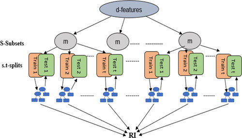
Draminski et al. (2008) provided an algorithm called MCFS for feature selection by ranking each attribute or feature in terms of their relative importance or discrimination in high-dimensional data problems. According to this algorithm, classification trees may declare a feature more important. The features importance (Relative Importance (RI)) was determined by building many trees for randomly chosen subsets (Niaz et al. 2020 ). For detail description, let d denotes the number of features, m is the number of randomly selected fixed features in each subset denoted by s and t represent the number of constructed trees for every s. Furthermore, we split every set s into training and test parts, then t trees are trained and validated. The relative importance of each feature, say f_k was measured by $${RI}_{fk}={\sum }_{\gamma =1}^{s.t}{\mathit{wAcc}}_{\gamma }^u{\sum }_{n_{fk}\left(\gamma \right)}GR\left(n_{fk}\right(\gamma \left)\right){\left(\frac{No.\mathrm{ }in\mathrm{ }{n}_{fk}\left(\gamma \right)}{No.\mathrm{ }in\mathrm{ }\gamma }\right)}^v$$ where, ${\mathit{wAcc}}_{\gamma }^u$ is the weighted accuracy over $\gamma$’s trees, $GR(n_{fk}(\gamma ))$ denotes the gain ratio for tree nodes, $No.\mathit{\text{ in }}{n}_{fk}(\gamma )$ is the number of samples in the node $n_{fk}(\gamma )$ and $No.\mathit{\text{ in γ}}$ is the number of samples in the root of ${\gamma }^{th}$ tree. The values of three parameters, m, s and t were prespecified by a practitioner and set u = v = 1. For the main step procedure, overall s.t trees are generated, where s and t would be so large that every feature has a chance of being appeared in many different subsets. For more details, see Figure 1.

Figure 1. Monte Carlo Feature Selection algorithm flow chart.

2.5. Non-homogeneous Poisson process

The non-homogeneous Poisson process models are the widely used models for the analysis of counting processes (failure or event occurrence, reliabilities) and to analyse the rate of change of a process (Guler Dincer et al. 2022; Liu and Xie 2022). Thaduri (2020) utilized the NHPP model to estimate the probabilities for rerouting traffic using TMS. This study analysed life data from a growth curve to calculate the mean number of repairs and the rate of failure occurrence. The goal was to predict the nowcast for the present working condition. Al-Dousari et al. (2021) conducted a comparative study of NHPP models. They utilized appropriate models to analyse the rate of change in the process and predictions of COVID-19 confirmed cases, recoveries and deaths. The counting process $M\left(t\right), t\ge 0,$ is a stochastic process as it is non-decreasing, integer-valued, and non-negative for all $t\ge 0.$ Let $M\left(t\right)$ is the number of events that occurred during time t, then $M\left(t, t+h\right),$ is the number of events that occurred during the time interval $\left[t, t+h\right], h\ge 0$ and can be presented as $M\left(t, t+h\right)=M\left(t+h\right)-M(t).$ The counting process having independent event occurrence in non-overlapping time intervals has independent increments, ie has stationary increments if the distribution of the number of events occurred during the time interval $\left[t, t+h\right],$ depends on the time interval. In other words, $M\left(t\right)$ is a Poisson random variable having intensity function $\lambda (t)$ varying over time, is a NHPP with mean value function $\mu \left(t\right)=E\left(M\left(t\right)\right)$ and $\lambda \left(t\right)=\frac{\partial }{\partial t}\mu \left(t\right).$ For the interval $\left[t, t+h\right],$ the mean value function is $\left(t, t+h\right)=E\left(M\left(t+h\right)-M(t)\right)=E\left(M\left(t+h\right)\right)-E\left(M\left(t\right)\right)=\mathrm{ }\mu \left(t+h\right)-\mu \left(t\right),$ where, $\mu \left(t+h\right)$ is the mean value function at the time interval $\left[0, t+h\right].$ So, the probability mass function for the NHPP can be defined as: $$P\left(M\left(t,\mathrm{ }t+h\right)=k\right)=\frac{{\left(\mu \left(t,\mathrm{ }t+h\right)\right)}^k}{k!}\left(\exp \hspace{0.17em}\left(-\mu \left(t,\mathrm{ }t+h\right)\right)\right)$$ where, $k$ is the number of events that occurred at the time interval $\left[t, t+h\right].$

2.6. Bayesian estimation

The Markov Chain Monte Carlo (MCMC) simulation-based Bayesian inference estimation procedures, which incorporate prior distributions of model parameters, are the most efficient and effective methods for parameter estimation. NHPP models rely on intensity and mean value functions that include various hyperparameters. The estimation of these hyperparameters is based on the joint or marginal posterior distributions of these parameters, which are calculated using MCMC simulation algorithms based on Bayesian estimation procedures (Al-Dousari et al. 2021; de Oliveira Peres et al. 2022; Kim and Kottas 2022). For the mathematical description of the Bayesian estimation, let $\mathbf{\Theta }$ denote the parameters of the intensity function of the NHPP model, $P(\mathbf{\Theta })$ be the joint prior distribution of the parameters, $L(\mathbf{\Theta };{\mathbf{T}}_{\mathbf{k}})$ is the likelihood function of the model of interest, ${\mathbf{T}}_{\mathbf{k}}=\left(\mathrm{k};\mathrm{ }{\mathrm{t}}_1,\mathrm{ }{\mathrm{t}}_2,{\mathrm{t}}_3\dots \dots \dots {\mathrm{t}}_{\mathrm{k}};\mathrm{T}\right)$ is the data set having $k$ observed occurrence time ${\mathrm{t}}_1,\mathrm{ }{\mathrm{t}}_2,{\mathrm{t}}_3\dots \dots \dots {\mathrm{t}}_{\mathrm{k}}$ on a time interval T and $P(\mathbf{\Theta }/{\mathbf{T}}_{\mathbf{k}})$ is the joint posterior distribution for $\mathrm{\Theta }$ given the data ${\mathrm{T}}_{\mathrm{k}}$ for the time interval [0, T]. Mathematically, $$P\left(\mathbf{\Theta }/{\mathbf{T}}_{\mathbf{k}}\right)\propto \mathrm{ }P\left(\mathbf{\Theta }\right)L\left(\mathbf{\Theta };{\mathbf{T}}_{\mathbf{k}}\right)$$ $$L\left(\mathbf{\Theta };{\mathbf{T}}_{\mathbf{k}}\right)=\left(\prod _{i=1}^k\lambda \left(t_i\right)\right)\mathrm{e}\mathrm{xp}\left(\mu \right(T\left)\right)$$

The simulated samples for the $P\left(\mathbf{\Theta }/{\mathbf{T}}_{\mathbf{k}}\right)$ and the posterior summaries of interest are obtained for $\mathrm{\Theta }$ by utilizing the standard MCMC method, ie Gibbs sampling. Mostly, Gibbs sampling is initiated by providing initial values or generating the initial values of parameters from the prior distribution and then gradually converging to the target value. The Trace plots and some useful summary statistics are the frequently used techniques to check the convergence, and these results provide a clear indication of stabilized simulations. A library, ‘R2jags’ of R software introduced by Su et al. (2015), provides considerable simplifications in these calculations. A Bayesian adequacy model, Deviance Information Criteria (DIC), is considered to check the model’s suitability.

Root Mean Square Error (RMSE) can be calculated for estimated drought events to validate the fitted model’s performance for each cluster representative station. This is accomplished by comparing the observed drought events with those predicted by the model for each representative station. It delivers an understanding of the accuracy of the fitted model for each location and could help us identify the locations where the model may need improvement. Mathematically RMSE presented as $$\mathit{RMSE}=\sqrt{\frac{\sum _{i=1}^n{\left(\mathit{Observed}-\mathit{Predicted}\right)}^2}{n}}$$

Where, ‘Observed’ is the original data value, ‘Predicted’ is the fitted model estimated value and ‘n’ is the number of observation s.

2.7. Proposed framework algorithm

The proposed framework mainly focused on the regionally integrated clusters study. First, it distributes the observed meteorological stations of the region in the optimal number of homogenous clusters. Then it targets the single important and representative location for the drought events analysis of the respective cluster. The proposed framework mainly consists of three phases. The flowchart of the proposed framework is presented in Figure 2. Each step of the algorithm at each stage is as follows:

Figure 2. Flow chart of proposed framework.

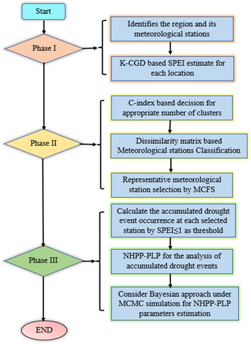
• Phase I: K-component Gaussian distribution-based SPEI calculation

1. Decide the study area and the meteorological stations to collect time series precipitation data.

2. Calculate the SPEI vector for each meteorological station by utilizing K-component Gaussian distribution in the standardization process, as discussed earlier in Section 2.1.

• Phase II: decision on the appropriate number of clusters using C-index, dissimilarity matrix-based classification of meteorological stations and MCFS-based identification of representative meteorological stations.

• 3. Utilize the method of C-index to identify the appropriate number of clusters for given data. The mathematical description for calculating C-index is provided in Section 2.2.

• 4. Utilize the clustering scheme based on the dissimilarity matrix and use the Euclidian distance measures to calculate the dissimilarity matrix. Section 2.2 provides a detailed mathematical description of clustering.

• 5. Utilize the MCFS algorithm to identify representative meteorological stations in each cluster based on their relative importance in the cluster. For the mathematical description and algorithm details, see Section 2.3.

• Phase III: Drought events analysis using NHPP and the estimation of model parameters under Gibbs sampling

1. The Poisson events of interest are the months the SPEI measurement has exceeded a given interest threshold. Here, $\mathit{SPEI}\le -1$ is the threshold of interest and considers the drought event occurrence (ie observed drought event) for each such month in the time.

2. The threshold corresponds to the overall average measurement of SPEI for each meteorological station. So, based on our interest, the number of times the monthly SPEI values exceed their threshold over a given time interval is a counting process, particularly NHPP. It allows calculating the probability of the number of drought events and the rate of change of drought event occurrences in a given time interval.

3. Consider the NHPP, ie Power Law Process (PLP) model, to study the accumulated number of drought event occurrence months at each representative meteorological station of the clusters for any time interval in the given period. The intensity and mean value function parametric forms depending on time and on unknown parameters assumed for the NHPP are $\lambda \left(t\right)=\left(\frac{a}{b}\right){\left(\frac{t}{b}\right)}^{a-1}$ and $\mu \left(t\right)={\left(\frac{t}{b}\right)}^a, a \& b \in \left(0, \infty \right), t\ge 0.$

4. The statistical analysis for estimating NHPPs parameters considers the hierarchical Bayesian approach with non-informative priors of model parameters under MCMC simulation methods (ie Gibbs sampling) to get the posterior summaries of interest. We further assume prior independence among the parameters and the appropriateness of models for each representative meteorological station of each cluster using Deviance Information Criteria (DIC).

3. Application

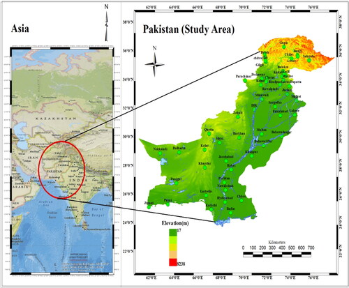
Globally, the agricultural and economic sectors of various countries are influenced due to the adverse effects of climate change; Pakistan is one of those highly affected countries. Pakistan is facing many challenges of water deficiency and water contamination. Almost all regions of the country are affected due to unbalance and irregular behavior of the precipitation. Especially in Sindh and southern Punjab, several human deaths and livestock destruction have been reported in the last three decades. So, it is necessary to strengthen the monitoring of precipitation patterns, drought monitoring and the generation of effective mitigation policies for early warnings by developing and collecting efficient and accurate monitoring frameworks and tools (Tehreem et al. 2022). To evaluate the proposed framework strength, efficacy and efficiency, time series precipitation and temperature (minimum & maximum) data from various meteorological stations dispersed throughout Pakistan have been considered. The monthly average precipitation, minimum temperature and maximum temperature data from January 1968 to December 2016 were collected from the Pakistan meteorological department. The study area and the observed locations are presented in Figure 3.

Figure 3. Study area with observed meteorological stations.

4. Results

At the initial stage of the proposed framework, the modified SPEI based on GMD is estimated. The scatter plots and histograms of theoretical and empirical CDF of K-CGMD for water deficit values were calculated from temperature and precipitation data sets. The CDFs for each station are utilized to standardize Water deficit values ‘D’ for calculating SPEI values. Figure 4 presents the scatter plots and histograms of theoretical and empirical CDF for Cherat, Kakul, DIK and Darosh. Table 1 presents the K-CGMD Bayesian Information Criteria (BIC) values for selected stations. The small BIC values and QQ plots for each station indicated the appropriateness of 12-CGMD fitting and improved the accuracy of drought monitoring and its related analysis. The largest value of BIC is −5710.38 for Jiwani, and the smallest value of BIC is −6983.29 for Balakot. Figure 5 presents the temporal behavior of SPEI-1 for 49 years at Cherat, Kakul, DIK and Drosh. It clearly shows the variation in the annual pattern of SPEI-1 at each station, and these variations in the annual pattern differ from station to station. After calculating the SPEI-1 of the individual station, in Phase II, first, we generate the clusters of all 52 meteorological stations based on these calculated SPEI-1 values. Moreover, the optimal number of clusters is selected based on the C-index before generating the clusters. The number of clusters and their C-index values are given in Table 2. The minimum value of the C-index indicated that its corresponding number of clusters is optimal. The minimum value of the C-index is 0.5429, indicating that the optimal number of clusters is 9. The 52 stations are further distributed in 9 clusters based on their dissimilarity matrix calculated using the Euclidian distance. The list of meteorological stations corresponding to each cluster is presented in Table 3. The number of stations for each cluster varies, ie cluster 1, 2, 3, 4, 5, 6, 7, 8 and 9 has 4, 5, 4, 8, 2, 4, 12, 8 and 5 stations, respectively. Furthermore, the homogeneity within the cluster is analysed using the Pearson Chi-square test of homogeneity, with the null hypothesis being that the stations within clusters are homogeneous. The results of the Pearson chi-square test of homogeneity for each cluster are presented in Table 4, where the P-value for each cluster is ≥ 0.9976. It indicates that all the generated clusters are homogeneous, even though the number of stations varies in each cluster.

Figure 4. The scatter plots and Histogram of theoretical and empirical CDF of K-CGMD.

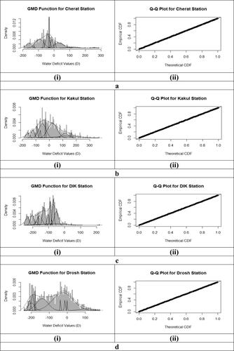
Figure 5. Time series plots of SPEI (a) Cherat (b) Kakul (c) DIK and (d) Drosh.

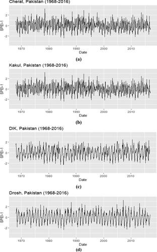
Table 1. K-CGMD BIC values for all observed stations.

Stations	BIC	Stations	BIC	Stations	BIC
Cherat	−6443.57	Nawabshah	−6120.31	Khanpur	−6097.13
Peshawar	−6503.37	Dalbadin	−6238.63	Lahore	−6568.35
Kakul	−6750.19	Panjgur	−6048.53	Rawalpindi	−6972.93
DIK	−6235.07	Pasni	−5773.71	Sargodha	−6362.13
Drosh	−6643.90	Kalat	−6266.78	Murree	−6958.54
Parachinar	−6573.81	Quetta	−6388.70	Mianwali	−6398.15
Kohat	−6409.03	Sibbi	−6198.63	Bahawalnagar	−6192.85
Risalpur	−6647.92	Jiwani	−5710.38	Gilgit	−6138.02
Balakot	−6983.29	Lasbella	−5986.49	Sakardu	−6327.74
Chitral	−6623.50	Zohub	−6131.86	Bunji	−6047.10
Dir	−6929.61	Nokkundi	−5934.32	Chilas	−6186.41
Hyderabad	−5994.85	Khuzdar	−6162.56	Astore	−6350.72
Jacobabad	−6161.84	Barkhan	−6107.76	Gupis	−6056.78
Padidan	−6105.77	Faisalabad	−6248.98	Kotli	−6906.54
Rohri	−6124.40	Jhelum	−6766.23	Muzaffarabad	−6911.58
Badin	−6064.86	Sialkot	−6881.34	Garhi Dupatta	−6903.76
Chhor	−6084.78	Bahawal Pur	−6097.37
Karachi	−5741.13	Multan	−6101.98

Table 2. The number of clusters and its calculated C-index values.

Number of clusters	C-index values	Number of clusters	C-index values
2	0.5617	7	0.5656
3	0.5458	8	0.5674
4	0.554	9	0.5429
5	0.5755	10	0.7227
6	0.6159

Table 3. Stations distribution for each cluster.

Cluster 1	Cluster 2	Cluster 3	Cluster 4	Cluster 5	Cluster 6	Cluster 7	Cluster 8	Cluster 9
Cherat	Kakul	DIK	Drosh	Parachinar	Hyderabad	Jacobabad	Dalbadin	Jhelum
Peshawar	Balakot	Faisalabad	Chitral	Dir	Badin	Padidan	Panjgur	Sialkot
Kohat	Murree	Sargodha	Gilgit		Chhor	Rohri	Kalat	Lahore
Risalpur	Muzaffarabad	Mianwali	Sakardu		Karachi	Nawabshah	Quetta	Rawalpindi
	GarhiDupatta		Bunji			Pasni	Sibbi	Kotli
			Chilas			Jiwani	Zohub
			Astore			Lasbella	Nokkundi
			Gupis			Barkhan	Khuzdar
						BahawalPur
						Multan
						Khanpur
						Bahawalnagar

Table 4. Pearson Chi-square test for homogeneity.

Cluster #	Degree of freedom	Chi-square statistics	p Value
1	18	3.7642	.9998
2	24	2.3733	1
3	18	1.8169	1
4	42	8.4088	1
5	6	0.51555	.9976
6	18	3.8027	.9998
7	66	10.036	1
8	42	4.9166	1
9	24	1.4295	1

The MCFS algorithm provides the ranked list based on the relative importance of each station in each cluster. Table 5 presents the relative importance values for stations of each cluster except cluster 5 because it has only two stations, and the MCFS is unsuitable for such small clusters. The most important stations for Cluster 1 to 4 are Peshawar, Muzaffarabad, DIK and Chitral, with relative importance values of 0.4234, 0.2381, 0.5190 and 0.6660. The least important stations for clusters 1 to 4 are Cherat, Murree, Sargodha and Astore, with relative importance values of 0.2187, 0.1973, 0.3442 and 0.1560. Similarly, the most important stations for Clusters 6 to 9 are Hyderabad, Rohri, Nokkundi and Lahore, with relative importance values of 0.7748, 0.7536, 1.2512 and 0.5373, respectively. The least important stations for clusters 6 to 9 are Karachi, Barkhan, Zohub and Kotli, with relative importance values of 0.3845, 0.1436, 0.1380 and 0.1939. The important stations of each cluster are selected and utilized for the analysis of drought events. Based on the climate moisture categories in Liu et al. (2021), drought events are considered or observed for the month having SPEI≤-1. For months with a Standardized Precipitation-Evapotranspiration Index (SPEI) value of ≤ −1, the months in which drought events occur are considered as the observed drought events at each representative station. The accumulated number of observed drought events for time ‘T’ is the total number of months having $\mathit{SPEI}\le -1$ till that time.

Table 5. MCFS based estimated Relative importance (RI) for the stations in each cluster.

Cluster 1		Cluster 2		Cluster 3		Cluster 4
Stations	Relative importance	Stations	Relative importance	Stations	Relative importance	Stations	Relative importance
Peshawar	0.4234	Muzaffarabad	0.2381	DIK	0.5190	Chitral	0.6660
Risalpur	0.3988	Balakot	0.2228	Faisalabad	0.4254	Gilgit	0.6419
Kohat	0.2392	Kakul	0.2163	Mianwali	0.3492	Sakardu	0.4072
Cherat	0.2187	GarhiDupatta	0.1986	Sargodha	0.3442	Bunji	0.4039
		Murree	0.1973			Chilas	0.3835
						Drosh	0.3170
						Gupis	0.2725
						Astore	0.1560
Cluster 6		Cluster 7		Cluster 8		Cluster 9
Stations	Relative importance	Stations	Relative importance	Stations	Relative importance	Stations	Relative importance
Hyderabad	0.7748	Rohri	0.7536	Nokkundi	1.2512	Lahore	0.5373
Badin	0.6726	Padidan	0.7109	Dalbadin	0.7487	Sialkot	0.4626
Chhor	0.5322	Jacobabad	0.6565	Quetta	0.5009	Jhelum	0.4462
Karachi	0.3845	Nawabshah	0.6486	Sibbi	0.4668	Rawalpindi	0.2927
		Khanpur	0.6442	Panjgur	0.3912	Kotli	0.1940
		BahawalPur	0.2981	Kalat	0.3090
		Pasni	0.2977	Khuzdar	0.1663
		Multan	0.2883	Zohub	0.1380
		Jiwani	0.2696
		Lasbella	0.2468
		Bahawalnagar	0.2078
		Barkhan	0.1436

The Bayesian analysis for the NHPP-PLP model is conducted under MCMC simulation, and the Posterior summaries of interest are presented in Table 6, along with the DIC values for each important station and the two stations of cluster 5 (10 selected important stations). For all these stations, the values of MC errors and standard deviations are small enough. It is assumed that the prior distribution of ‘a’ and ‘b’ is Uniform(0, 100]. The marginal posterior densities of the hyperparameters (a,b) and their trace plots for each station are presented in Figure 6. These plots are presented to observe the convergence in the process. The burn-in sample of size 5000 was considered to eliminate the effect of the initial values. The results for marginal posterior distributions with Monte Carlo estimates for DIC are generated based on 25,000 simulated Gibbs samples. The estimated parameter values for the NHPP-PLP model of each station are utilized to estimate the cumulative drought events over the time in the study time for Peshawar, Muzaffarabad, DIK, Chitral, Dir, Parachinar, Hyderabad, Rohri, Nokkundi and Lahore. The observed accumulative drought events over time and the estimated drought events for each station are presented in Figure 7, and the Mean Square Error for each station is provided in Table 7. In NHPP model validation results, the MSE values for Peshawar, Muzaffarabad, DIK, Chitral, Dir, Parachinar, Hyderabad, Rohri, Nokkundi & Lahore are 2.765, 6.104, 1.709, 1.675, 6.071, 12.954, 1.316, 2.804, 1.595 and 0.994. Generally, the results revealed that the PLP model performed efficiently in predicting drought events over time, but its performance is not as effective in Cluster 5(see Figure 7 ei & eii).

Figure 6. NHPP model parameters marginal posterior density and trace plots for each station.

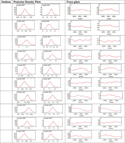
Figure 7. Accumulated number of drought events at each representative station of each cluster (a) cluster 1, (b) cluster 2, (c) cluster 3, (d) cluster 4, (e i ii) cluster 5, (f) cluster 6, (g) cluster 7, (h) cluster 8 and (i) cluster (9).

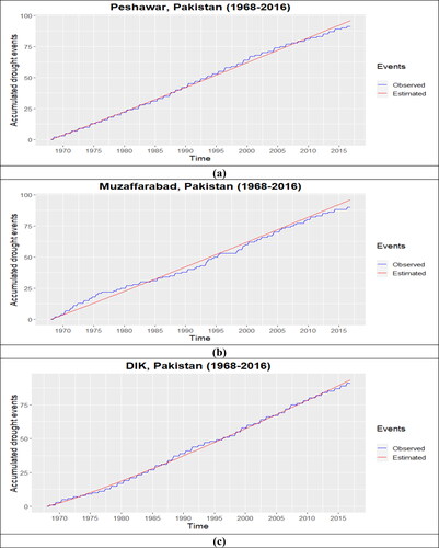
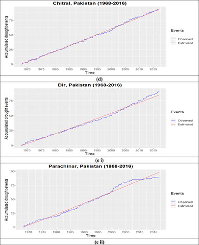
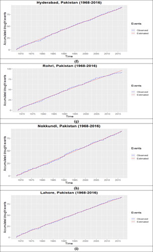
Table 6. NHPP model parameters MCMC summary statistics for the representative station of each cluster.

Stations	Parameters	Mean	Standard deviation	MC error	95% C.I	DIC
Peshawar	a	1.034	0.012	6.681E-04	[1.01, 1.058]	3199.36
	b	7.121	0.338	1.819E-02	[6.472, 7.788]
Muzaffarabad	a	0.914	0.011	5.657E-04	[0.8932, 0.9355]	3297.94
	b	4.342	0.230	1.192E-02	[3.917, 4.804]
DIK	a	1.150	0.013	6.719E-04	[1.125, 1.176]	3137.21
	b	11.390	0.449	2.335E-02	[10.52, 12.3]
Chitral	a	1.039	0.012	6.147E-04	[1.016, 1.063]	3181.99
	b	7.471	0.342	1.726E-02	[6.825, 8.147]
Dir	a	1.052	0.013	6.815E-04	[1.027, 1.078]	3204.77
	b	8.690	0.407	2.116E-02	[7.925, 9.5]
Parachinar	a	1.042	0.012	6.245E-04	[1.02, 1.066]	3349.71
	b	7.224	0.325	1.709E-02	[6.626, 7.895]
Hyderabad	a	0.922	0.012	6.574E-04	[0.8981, 0.9443]	3241.96
	b	4.499	0.250	1.403E-02	[4.006, 4.991]
Rohri	a	0.913	0.011	6.295E-04	[0.8905, 0.9353]	3284.41
	b	3.952	0.224	1.226E-02	[3.523, 4.395]
Nokkundi	a	1.016	0.012	6.438E-04	[0.9932, 1.041]	3174.53
	b	7.071	0.334	1.775E-02	[6.453, 7.754]
Lahore	a	0.917	0.011	6.407E-04	[0.8944, 0.9393]	3233.21
	b	4.316	0.238	1.335E-02	[3.868, 4.801]

Table 7. NHPP model validation result.

Station	RMSE	Station	RMSE
Peshawar	2.765	Parachinar	12.954
Muzaffarabad	6.104	Hyderabad	1.316
DIK	1.709	Rohri	2.804
Chitral	1.675	Nokkundi	1.595
Dir	6.071	Lahore	0.994

5. Discussion

Researchers and climatologists have introduced various drought indices, but standardized drought indices are the most frequently used drought indices (Tigkas et al. 2016; Ali et al. 2020; Harisuseno 2020; Liu et al. 2021; Niaz et al. 2021a, 2022b, 2022e, 2022f; Sein et al. 2021; Babre et al. 2022). The probability distribution fitting during standardization is the main issue in accurately calculating standardized drought indices. This issue was addressed by Ali et al. (2021), who introduced the K-CGMD fitting in standardization. It significantly improved the values of standardized drought indices. Therefore, in our study, during the calculation of SPEI, 12-CGMD is utilized for standardizing and fitting the distribution of Water deficit values. The R library ‘mixtools’, introduced by Benaglia et al. (2009) for the mixture model, are used for K-CGMD fitting. The BIC values of the fitted GMD at each station, the density plots and QQ plots provided significant insights into the accuracy of fitting the distributions. The time series plots of modified SPEI for randomly selected four stations are also provided in the study. Although the drought index SPEI is widely used that combines the temperature and precipitation data to provide a standardized measure of water availability, it assumes that the relationship between temperature and precipitation is constant over time. But in some regions, this relationship may depend on other factors, particularly in such areas; the fluctuation in the relationship of precipitation and temperature significantly impacts water availability and may lead to inaccurate estimates (Zaki and Noda 2022). The major factors affecting water availability are precipitation, evapotranspiration, land surface characteristics, humidity, wind speed and climate change (Mukherjee et al. 2018; Rehana et al. 2021). But SPEI ignored some significant variables and were not considered in calculating water availability. However, the SPEI is recommended as an alternative to SPI because it quantifies anomalies in accumulated climatic water balance, incorporating potential evapotranspiration to investigate drought events (Tefera et al. 2019).

Clustering of meteorological stations may help in developing more accurate drought monitoring and early warning systems. It also helps to establish localized drought management strategies (Feeny 2017). By analysing the specific cluster, it is possible to identify the areas particularly exposed to drought and get targeted interventions that are altered to the specific needs of those societies (Aladaileh et al. 2019). Therefore in our study, clusters of all 52 meteorological stations based on their time series data of SPEI are obtained using hierarchical clustering. The decision of the optimal number of clusters is decided using C-index. The minimum value of the C-index indicates the optimal number of clusters of 52 meteorological stations in the study area. The optimal number of clusters is 9, with a minimum value of C-index, ie 0.5429. After generating nine homogeneous clusters, a test for homogeneity indicates that the stations within each cluster exhibit homogeneity. In the next step of the proposed framework, the main target is to obtain the important representative station in each cluster. For this purpose, the MCFS technique provides an efficient and effective way to select each cluster’s important station. The stations are ranked based on their relative importance for each cluster. The selected relatively important stations enable us to assign the correct decision regarding drought severity conditions to each cluster every month for 49 years. To implement the last phase, the threshold of $\mathrm{SPEI}\le -1.0$ are used to obtain the vector of accumulated drought events that occurred at the selected 10 important stations. The PLP-based NHPP model is utilized to investigate the drought occurrence rate and estimate the drought events over time. For the Bayesian analysis, we assume that the prior distribution of ‘a’ and ‘b’ is uniform with the range (0, 100] along with the prior independence among the parameters. The Monte Carlo error indicates that the margin of error is very small when using the MCMC samples to estimate the posterior means for each parameter at each station. Therefore, the means of marginal posterior distributions of the parameters at each important and cluster-representative station are used to estimate the drought events over time and the rate of change of drought event occurrence. At the end of our study, the estimated over-observed drought events and the RMSE for each station showed that for Peshawar, DIK, Chitral, Hyderabad, Rohri, Nokkundi and Lahore, the PLP model performed well, for Muzaffarabad and Dir it performs average, but for Parachinar, it performs worst due to some abrupt changes occurred during the time.

6. Conclusion

The current study proposes a generalized framework for quantifying and monitoring meteorological drought severity. The performance of the proposed framework is validated and assessed for 52 stations in Pakistan. The modified and improved SPEI based on GMD is estimated in the proposed framework. The recommended clustering method in the farmwork efficiently produced various homogeneous clusters, and MCFS performs well in selecting important representative stations for each cluster. The Bayesian-based approach MCMC simulation is utilized to fit the NHPP-PLP model to estimate average drought events along its rate of change of events occurrence. DIC values for MCMC-based NHPP-PLP model parameters estimation and the RMSEs for the fitted NHPP-PLP model indicate the accuracy and significance, respectively. The outcomes of the proposed framework effectively quantify and monitor the severity of meteorological drought. Therefore the proposed framework for spatiotemporal assessment of drought events and their severity is a significant addition to the literature that helps the decision-makers to understand the effects of drought occurrences better and implement their drought mitigation policies to reduce the losses caused by it. The framework can further be improved by adding new climatological variables to calculate the indices to that quantify and monitor the severity of meteorological drought.

Ethics statement

All procedures followed were in accordance with the ethical standards with the Helsinki Declaration of 1975, as revised in 2000.

Consent form

All authors are agreed to for publication, there is no legal constraint in publishing the data used in the manuscript. All authors are voluntarily agreed to participate in this research

Authors contribution

All authors contributed equally.

Disclosure statement

No potential conflict of interest was reported by the author(s).

Data availability statement

The data and codes used for the preparation of the manuscript are available with the corresponding author and can be provided upon request.

Additional information

Funding

This work was supported by the Deanship of Scientific Research at King Khalid University through Large Groups Research Project under grant number (RGP.2/23/44). And this study is supported via funding from Prince Sattam bin Abdulaziz University project number (PSAU/2023/R/1444).

References

- Aladaileh H, Al Qinna M, Karoly B, Al-Karablieh E, Rakonczai J. 2019. An investigation into the spatial and temporal variability of the meteorological drought in Jordan. Climate. 7(6):82. doi: 10.3390/cli7060082.
- Alahacoon N, Amarnath G. 2022. Agricultural drought monitoring in Sri Lanka using multisource satellite data. Adv Space Res. 69(11):4078–4097. doi: 10.1016/j.asr.2022.03.009.
- Alahacoon N, Edirisinghe M. 2022. A comprehensive assessment of remote sensing and traditional based drought monitoring indices at global and regional scale. Geomatics Nat Hazards Risk. 13(1):762–799. doi: 10.1080/19475705.2022.2044394.
- Al-Dousari A, Ellahi A, Hussain I. 2021. Use of non-homogeneous Poisson process for the analysis of new cases, deaths, and recoveries of COVID-19 patients: a case study of Kuwait. J King Saud Univ Sci. 33(8):101614. doi: 10.1016/j.jksus.2021.101614.
- Ali Z, Ellahi A, Hussain I, Nazeer A, Qamar S, Ni G, Faisal M. 2021. Reduction of errors in hydrological drought monitoring–a novel statistical framework for spatio-temporal assessment of drought. Water Resour Manage. 35(13):4363–4380. doi: 10.1007/s11269-021-02952-x.
- Ali Z, Hussain I, Faisal M, Almanjahie IM, Ahmad I, Khan DM, Grzegorczyk M, Qamar S. 2019. A probabilistic weighted joint aggregative drought index (PWJADI) criterion for drought monitoring systems. Tellus A Dyn Meteorol Oceanogr. 71(1):1588584. doi: 10.1080/16000870.2019.1588584.
- Ali Z, Hussain I, Faisal M, Khan DM, Niaz R, Elashkar EE, Shoukry AM. 2020. Propagation of the multi-scalar aggregative standardized precipitation temperature index and its application. Water Resour Manage. 34(2):699–714. doi: 10.1007/s11269-019-02469-4.
- Ali Z, Hussain I, Faisal M, Nazir HM, Moemen MAE, Hussain T, Shamsuddin S. 2017. A novel multi-scalar drought index for monitoring drought: the standardized precipitation temperature index. Water Resour Manage. 31(15):4957–4969. doi: 10.1007/s11269-017-1788-1.
- Anshuka A, van Ogtrop FF, Willem Vervoort R. 2019. Drought forecasting through statistical models using standardised precipitation index: a systematic review and meta-regression analysis. Nat Hazards. 97(2):955–977. doi: 10.1007/s11069-019-03665-6.
- Asmall T, Abrams A, Röösli M, Cissé G, Carden K, Dalvie MA. 2021. The adverse health effects associated with drought in Africa. Sci Total Environ. 793:148500. doi: 10.1016/j.scitotenv.2021.148500.
- Babre A, Kalvāns A, Avotniece Z, Retiķe I, Bikše J, Jemeljanova KPM, Zelenkevičs A, Dēliņa A. 2022. The use of predefined drought indices for the assessment of groundwater drought episodes in the Baltic States over the period 1989–2018. J Hydrol Reg Stud. 40:101049.
- Benaglia T, Chauveau D, Hunter DR, Young DS. 2009. mixtools: an R package for analyzing mixture models. J Stat Soft. 32(6):1–29. doi: 10.18637/jss.v032.i06.
- Charrad M, Ghazzali N, Boiteau V, Niknafs A. 2014. NbClust: an R package for determining the relevant number of clusters in a data set. J Stat Soft. 61(6):1–36. doi: 10.18637/jss.v061.i06.
- Chen Q, Sang L. 2018. Face-mask recognition for fraud prevention using Gaussian mixture model. J Vis Commun Image Represent. 55:795–801. doi: 10.1016/j.jvcir.2018.08.016.
- de Oliveira Peres MV, de Oliveira RP, Achcar JA, Nunes AA. 2022. Case-fatality rate by Covid-19: a hierarchical Bayesian analysis of countries in different regions of the world. Braz J Biom. 40(2). doi: 10.28951/bjb.v40i2.565.
- Dibi-Anoh PA, Koné M, Gerdener H, Kusche J, N’Da CK. 2023. Hydrometeorological extreme events in West Africa: droughts. Surv Geophys. 44(1):173–195. doi: 10.1007/s10712-022-09748-7.
- Draminski M, Rada-Iglesias A, Enroth S, Wadelius C, Koronacki J, Komorowski J. 2008. Monte Carlo feature selection for supervised classification. Bioinformatics. 24(1):110–117. doi: 10.1093/bioinformatics/btm486.
- Ellahi A, Almanjahie IM, Hussain T, Hashmi MZ, Faisal S, Hussain I. 2020. Analysis of agricultural and hydrological drought periods by using non-homogeneous Poisson models: linear intensity function. J Atmos Sol Terr Phys. 198:105190. doi: 10.1016/j.jastp.2020.105190.
- Ellahi A, Hussain I, Hashmi MZ, Almazah MMA, Al-Duais FS. 2021. Agricultural drought periods analysis by using non-homogeneous Poisson models and regionalization of appropriate model parameters. Tellus A Dyn Meteorol Oceanogr. 73(1):1948241. doi: 10.1080/16000870.2021.1948241.
- Feeny E. 2017. From early warning to early action in Somalia: what can we learn to support early action to mitigate humanitarian crises?. Oxford, UK: Oxfam; p. 44.
- Guler Dincer N, Demir S, Yalçin MO. 2022. Forecasting COVID19 reliability of the countries by using non-homogeneous Poisson process models. New Gener Comput. 40(4):1143–1164. doi: 10.1007/s00354-022-00183-1.
- Harisuseno D. 2020. Comparative study of meteorological and hydrological drought characteristics in the Pekalen River Basin, East Java, Indonesia. J Water Land Dev. 45(IV–VI):29–41. doi: 10.24425/jwld.2020.133043.
- Jiménez-Donaire MDP, Tarquis A, Giráldez JV. 2020. Evaluation of a combined drought indicator and its potential for agricultural drought prediction in southern Spain. Nat Hazards Earth Syst Sci. 20(1):21–33. doi: 10.5194/nhess-20-21-2020.
- Kafy AA, Bakshi A, Saha M, Al Faisal A, Almulhim AI, Rahaman ZA, Mohammad P. 2023. Assessment and prediction of index based agricultural drought vulnerability using machine learning algorithms. Sci Total Environ. 867:161394. doi: 10.1016/j.scitotenv.2023.161394.
- Kim H, Kottas A. 2022. Erlang mixture modeling for Poisson process intensities. Stat Comput. 32(1):1–15. doi: 10.1007/s11222-021-10064-0.
- Kron W, Löw P, Kundzewicz ZW. 2019. Changes in risk of extreme weather events in Europe. Environ Sci Policy. 100:74–83. doi: 10.1016/j.envsci.2019.06.007.
- Liu C, Yang C, Yang Q, Wang J. 2021. Spatiotemporal drought analysis by the standardized precipitation index (SPI) and standardized precipitation evapotranspiration index (SPEI) in Sichuan Province, China. Sci Rep. 11(1):1280. doi: 10.1038/s41598-020-80527-3.
- Liu X, Xie N. 2022. Grey-based approach for estimating software reliability under non-homogeneous Poisson process. J Syst Eng Electron. 33(2):360–369. doi: 10.23919/JSEE.2022.000038.
- McKee TB, Doesken NJ, Kleist J. 1993. The relationship of drought frequency and duration to time scales. Proceedings of the 8th Conference on applied climatology. Boston (MA): American Meteorological Society, Vol. 17, pp. 179–183.
- Mishra A, Alnahit A, Mukherjee S. 2022. Rainfall and droughts. In: Rainfall. Elsevier; p. 451–474.
- Moazzam MFU, Rahman G, Munawar S, Farid N, Lee BG. 2022. Spatiotemporal rainfall variability and drought assessment during past five decades in South Korea using SPI and SPEI. Atmosphere. 13(2):292. doi: 10.3390/atmos13020292.
- Mukherjee S, Mishra A, Trenberth KE. 2018. Climate change and drought: a perspective on drought indices. Curr Clim Change Rep. 4(2):145–163. doi: 10.1007/s40641-018-0098-x.
- Niaz R,Almanjahie IM,Ali Z,Faisal M,Hussain I. 2020. A novel framework for selecting informative meteorological stations using Monte Carlo feature selection (MCFS) algorithm. Adv. Meteorol. 2020:1–13. doi: 10.1155/2020/5014280.
- Niaz R,Almazah MM,Hussain I,Faisal M,Al-Rezami AY,Naser MA. 2022a. A new comprehensive approach for regional drought monitoring. PeerJ. 10:e13377. doi: 10.7717/peerj.13377.
- Niaz R, Almazah MM, Al-Duais FS, Iqbal N, Khan DM, Hussain I. 2022e. Spatiotemporal analysis of meteorological drought variability in a homogeneous region using standardized drought indices. Geomatics Nat Hazards Risk. 13(1):1457–1481. doi: 10.1080/19475705.2022.2079429.
- Niaz R, Almazah MM, Hussain I, Ali Z, Hussain A, Al-Rezami AY. 2023a. Proposing a new framework for analyzing the severity of meteorological drought. Geocarto Int. 38(1):2197512. doi: 10.1080/10106049.2023.2197512.
- Niaz R, Almazah MM, Hussain I, Filho JDP. 2021b. A new framework to substantiate the prevalence of drought intensities. Theor Appl Climatol. 147(3-4):1079–1090. doi: 10.1007/s00704-021-03876-7.
- Niaz R, Almazah M, Zhang X, Hussain I, Faisal M. 2021a. Prediction for various drought classes using spatiotemporal categorical sequences. Complexity. 2021:1–11. doi: 10.1155/2021/7145168.
- Niaz R, Hussain A, Almazah MM, Hussain I, Ali Z, Al-Rezami AY. 2023b. Identifying inter-seasonal drought characteristics using binary outcome panel data models. Geocarto International. 38(1):1–21. doi: 10.1080/10106049.2023.2178527.
- Niaz R, Iqbal N, Al-Ansari N, Hussain I, Elsherbini Elashkar E, Shamshoddin Soudagar S, Gani SH, Mohamd Shoukry A, Sh Sammen S. 2022c. A new spatiotemporal two-stage standardized weighted procedure for regional drought analysis. PeerJ. 10:e13249. doi: 10.7717/peerj.13249.
- Niaz R, Raza MA, Almazah MM, Hussain I, Al-Rezami AY, Al-Shamiri MMA. 2022b. Proportional odds model for identifying spatial inter-seasonal propagation of meteorological drought. Geomatics Nat Hazards Risk. 13(1):1614–1639. doi: 10.1080/19475705.2022.2095934.
- Niaz R, Tanveer F, Almazah M, Hussain I, Alkhatib S, Al-Razami AY. 2022d. Characterization of meteorological drought using Monte Carlo feature selection and steady-state probabilities. Complexity. 2022:1–19. doi: 10.1155/2022/1172805.
- O’Connor P, Murphy C, Matthews T, Wilby RL. 2022. Historical droughts in Irish catchments 1767–2016. Int J Climatol. 42(11):5442–5466. doi: 10.1002/joc.7542.
- Orimoloye IR. 2022. Agricultural drought and its potential impacts: enabling decision-support for food security in vulnerable regions. Front Sustain Food Syst. 6:15. doi: 10.3389/fsufs.2022.838824.
- Oyounalsoud MS, Najah A, Yilmaz AG, Abdallah M, Siddique M. 2022. Meteorological drought assessment in Sharjah, UAE using drought indices. Int J Environ Sci Dev. 13(1):16–20. doi: 10.18178/ijesd.2022.13.1.1366.
- Prabakaran I, Wu Z, Lee C, Tong B, Steeman S, Koo G, Zhang PJ, Guvakova MA. 2019. Gaussian mixture models for probabilistic classification of breast cancer. Cancer Res. 79(13):canres-0573–3502. doi: 10.1158/0008-5472.CAN-19-0573.
- Rehana S,Sireesha Naidu G,Monish NT, Sowjanya U. 2021. Modeling hydro-climatic changes of evapotranspiration over asemi-arid river basin of India. Journal of Water and Climate Change. 12(2):502 –520. doi: 10.2166/wcc.2020.173.
- Sein ZMM, Zhi X, Ogou FK, Nooni IK, Lim Kam Sian KT, Gnitou GT. 2021. Spatio-temporal analysis of drought variability in Myanmar based on the standardized precipitation evapotranspiration index (SPEI) and its impact on crop production. Agronomy. 11(9):1691. doi: 10.3390/agronomy11091691.
- Shah D, Shah HL, Dave HM, Mishra V. 2021. Contrasting influence of human activities on agricultural and hydrological droughts in India. Sci Total Environ. 774:144959. doi: 10.1016/j.scitotenv.2021.144959.
- Shorachi M, Kumar V, Steele-Dunne SC. 2022. Sentinel-1 SAR backscatter response to agricultural drought in the Netherlands. Remote Sens. 14(10):2435. doi: 10.3390/rs14102435.
- Siena M, Recalcati C, Guadagnini A, Riva M. 2023. A Gaussian-mixture based stochastic framework for the interpretation of spatial heterogeneity in multimodal fields. J Hydrol. 617:128849. doi: 10.1016/j.jhydrol.2022.128849.
- Su YS, Yajima M, Su MYS, SystemRequirements JAGS. 2015. Package ‘R2jags’. R package version 0.03-08. http://CRAN. R-project.org/package=R2jags.
- Tefera AS, Ayoade JO, Bello NJ. 2019. Comparative analyses of SPI and SPEI as drought assessment tools in Tigray Region, Northern Ethiopia. SN Appl Sci. 1(10):1–14. doi: 10.1007/s42452-019-1326-2.
- Tehreem Z, Ali Z, Al-Ansari N, Niaz R, Hussain I, Sammen SS. 2022. A novel appraisal protocol for spatiotemporal patterns of rainfall by reconnaissance the precipitation concentration index (PCI) with global warming context. Math Prob Eng. 2022:1–9. doi: 10.1155/2022/3012100.
- Thaduri A. 2020. Nowcast models for train delays based on the railway network status. Int J Syst Assur Eng Manag. 11(S2):184–195. doi: 10.1007/s13198-020-01002-w.
- Tigkas D, Vangelis H, Tsakiris G. 2016. Introducing a modified reconnaissance drought index (RDIe) incorporating effective precipitation. Proc Eng. 162:332–339. doi: 10.1016/j.proeng.2016.11.072.
- Tirivarombo S, Osupile D, Eliasson P. 2018. Drought monitoring and analysis: standardised precipitation evapotranspiration index (SPEI) and standardised precipitation index (SPI). Phys Chem Earth Parts A/B/C. 106:1–10. doi: 10.1016/j.pce.2018.07.001.
- Vélez-Nicolás M, García-López S, Ruiz-Ortiz V, Zazo S, Molina JL. 2022. Precipitation variability and drought assessment using the SPI: application to long-term series in the strait of Gibraltar area. Water. 14(6):884. doi: 10.3390/w14060884.
- Vicente-Serrano SM, Beguería S, López-Moreno JI. 2010. A multiscalar drought index sensitive to global warming: the standardized precipitation evapotranspiration index. J Clim. 23(7):1696–1718. doi: 10.1175/2009JCLI2909.1.
- Wang JC, Yang YH, Wang HM, Jeng SK. 2015. Modeling the affective content of music with a Gaussian mixture model. IEEE Trans Affective Comput. 6(1):56–68. doi: 10.1109/TAFFC.2015.2397457.
- Wang Q, Zeng J, Qi J, Zhang X, Zeng Y, Shui W, Xu Z, Zhang R, Wu X, Cong J. 2021. A multi-scale daily SPEI dataset for drought characterization at observation stations over mainland China from 1961 to 2018. Earth Syst Sci Data. 13(2):331–341. doi: 10.5194/essd-13-331-2021.
- Xia X, Yang W, Ren J, Li Y, Zhan Y, Han B, Liu T. 2022. Pluralistic image completion with gaussian mixture models. Adv Neural Inf Process Syst. 35:24087–24100.
- Zaki MK, Noda K. 2022. A systematic review of drought indices in tropical Southeast Asia. Atmosphere. 13(5):833. doi: 10.3390/atmos13050833.
- Zeng J, Zhang R, Qu Y, Bento VA, Zhou T, Lin Y, Wu X, Qi J, Shui W, Wang Q. 2022. Improving the drought monitoring capability of VHI at the global scale via ensemble indices for various vegetation types from 2001 to 2018. Weather Clim Extremes. 35:100412. doi: 10.1016/j.wace.2022.100412.
- Zhang L, Song W, Song W. 2020. Assessment of agricultural drought risk in the Lancang-Mekong region, South East Asia. Int J Environ Res Public Health. 17(17):6153. doi: 10.3390/ijerph17176153.
- Zhao Q, Chen Q, Jiao M, Wu P, Gao X, Ma M, Hong Y. 2018. The temporal-spatial characteristics of drought in the Loess Plateau using the remote-sensed TRMM precipitation data from 1998 to 2014. Remote Sens. 10(6):838. doi: 10.3390/rs10060838.