Spatial-temporal dynamics of transboundary forest disturbance-recovery and its influencing factors in the central Himalayas

Abstract

Transboundary forests in the Himalayas are one of the world’s biodiversity hotspots, but exploring the patterns and influencing factors related to forest disturbance-recovery is still limited. In this study, we used a random forests model, a LandTrendr temporal segmentation algorithm and geographical detector to investigate the spatial and temporal evolution characteristics of forest disturbance and recovery and their influencing factors in the central Himalayas from 1995 to 2018. The results showed that forest disturbance was dominant (∼2.94 × 10⁴ km²) and greater than recovery (∼0.56 × 10⁴ km²). Both disturbance and recovery showed a significant decreasing trend (p < 0.01); disturbance occurred mainly at low elevations and the Gandaki basin, while recovery was in eastern Nepal. Disturbance rates were highest in Nepal (1.14%) and recovery rates in China (0.29%). The main influencing factors on forest dynamics were elevation, temperature and population. The interaction of all factors was synergistically enhanced.

Keywords:

• Forest disturbance
• forest recovery
• Himalayas
• LandTrendr
• GEE
• natural and anthropogenic factors

1. Introduction

Forest ecosystems occupy one third of the Earth’s land surface (UNEP and FAO 2020), and they play a crucial role in biodiversity conservation, terrestrial carbon cycling, and soil and water conservation (Gibson et al. 2011; Bustamante et al. 2016). Forests are the predominant component of terrestrial ecosystems and are considered essential to any climate change mitigation strategy necessary for human well-being (Vancutsem et al. 2021). The worldwide forests are currently in a state of constant change and these changes occur in diverse forms and trajectories (Sloan and Sayer 2015; Chen et al. 2019; Senf and Seidl 2020; Burrell et al. 2022). These changes can be attributed to both natural phenomena, such as drought (Allen et al. 2015) and wildfires (Bowman et al. 2020), as well as anthropogenic activities, including selective logging (Matricardi et al. 2020) and deforestation. In contrast, forests also recover through natural vegetation succession or anthropogenic forest management. Timely and accurate monitoring of dynamic changes (disturbance and recovery processes) in forest ecosystems and identification of change impact mechanisms are essential for regional ecological, environmental protection and sustainable development.

The Himalayan region has extensive forests, and the livelihoods of over 50 million people are sustained by various timber and non-timber forest resources (Verma et al. 2021). As a significant natural resource, forests contribute immensely to the region’s ecological, social, cultural and economic aspects (Rao and Pant 2001; Dhyani and Dhyani 2020). Indeed, previous studies have found that forest disturbance still occurs in these forested landscapes. For example, Cui et al. (2022) found an overall declining trend in forests since 1990 in the Gandaki River basin of the central Himalayas. Chakraborty et al. (2017) studied the forests of Kumaon district, North Akhand, India, and found that it is experiencing intensive forest fragmentation. Sahana et al. (2018) reported about 112.5 km² of forest ecosystem in Rudraprayag district, India, has been deforested in the last 25 years. In particular, the forests in the central Himalayas are experiencing an accelerating fragmentation process. (Rao and Pant 2001; Sharma et al. 2016). In addition, other studies showed that forest degradation in the Himalayas appears to be a more severe problem than deforestation (Nandy et al. 2011). Nevertheless, such studies are limited mainly because much of the evidence is based on case studies, small samples, or surveys of geographically narrow areas. So far, comprehensive quantitative information on forest dynamics is still lacking on larger scales. In addition, most studies have focused on deforestation and degradation in the Himalayas, and little is known about forest recovery. However, disturbance and recovery are often concurrent geographic processes, and simultaneously studying them provides a more comprehensive understanding of forest ecosystem processes (Da Cruz et al. 2021). Similarly, the extent, magnitude and trend of forest disturbance and recovery in the Himalayan region in recent decades are unknown due to the lack of support for dynamic analysis of long time series. Although forest maps of acceptable accuracy are currently available globally, data accuracy varies by region (Milodowski et al. 2017; Hamunyela et al. 2020). Especially in ecosystem conversion and mountain region spatially explicit data on forest resource dynamics are urgently required to meet the analysis of change impact mechanisms.

Satellite remote sensing provides a spatially continuous, highly consistent representation of the Earth’s surface, and it has become an important data source for monitoring forest dynamics (Boyd and Danson 2005). The entire archive of the Landsat series has been widely used for global and regional fine-scale forest change mapping due to its medium to high resolution, free availability and accessibility (Hansen et al. 2013). Supervised classification mapping based on machine learning has recently been extensively developed. Many existing studies have shown that machine learning methods such as random forests (RF), support vector machines (SVM), and artificial neural networks (ANN) are usually more generalizable and robust for land change detection than traditional classification schemes based on logistic regression, maximum likelihood (Gómez et al. 2016). Accurate and adequate training samples are challenging in machine learning supervised classification. Traditional sample extraction still has disadvantages such as time-consuming and laborious, limited training samples, uneven distribution, and difficulty in timely updating (Ghorbanian et al. 2020). Therefore, strategies for efficiently acquiring reliable samples to support time-series land cover mapping need to be further developed. Further, many remote sensing time series modeling approaches have been applied to evaluate forest changes. It is mainly based on pixel-level derived time trajectories to identify abrupt breakpoints and continuous trends. Some techniques that employ annual time series of spectral indices to distinguish disturbance due to abrupt changes as well as recovery including the Vegetation Change Tracker (VCT) model (Huang et al. 2010) and the Landsat-based detection of trends in disturbance and recovery (LandTrendr) algorithm (Kennedy et al. 2010). The Breaks for Additive Seasonal and Trend (BFAST) method (Verbesselt et al. 2010) and the Continuous Change Detection and Classification (CCDC) technique (Zhu and Woodcock 2014) are used to perform boundary estimates of seasonal and interannual trends, and any significant deviation from the boundary is detected as change.

The above methods have shown great potential in the past for detecting forest changes on a large scale. Still, the need for high storage and computational power and time-consuming operations have limited their implementation. In recent years, with the accelerated development of remote sensing cloud platforms, the rapid processing and storage of large-scale and long-term sequence satellite remote sensing images is no longer a problem. Among various cloud computing platforms, Google Earth Engine (GEE) has powerful computing efficiency and a considerable amount of geoscience data (Gorelick et al. 2017). In addition, among these algorithms, LandTrendr was initially developed in 2010 using interactive data language (IDL) software and later implemented in the Google Earth Engine (GEE) platform in 2018. This provides the ability to evaluate forest disturbance and recovery in terms of both time and cost effectiveness, particularly in inaccessible mountainous regions. The LandTrendr algorithm represents changes in pixel feature parameters, such as spectral values, as linear segments. The segmented results are further used to identify specific change events and capture related information, such as the year of change, duration of change, and magnitude of change. It not only captures long-term slow forest changes but also detects abrupt change trends, making it widely applicable (Zhu et al. 2019; Senf and Seidl 2020; Liu et al. 2023). For example, recent studies have demonstrated the effectiveness of LandTrendr in detecting disturbance and recovery in temperate, subtropical, and tropical forests (Shen et al. 2022; Wimberly et al. 2022).

Transboundary regions are areas close to or cross-national political boundaries that define countries and territories (Liu et al. 2020). The Himalayan forest is inherently transboundary and heterogeneous regarding governance systems and cultural and social diversity. In addition, as one of the 36 global biodiversity hotspots (Mittermeier et al. 2011), the Himalayan landscape has complex forest types and ecosystems (Zhang et al. 2020). Forest change is usually caused by a combination of direct causes and underlying forces (Verma et al. 2021). As globalization advances, national borders and frontier areas can be transformed into urban agglomerations with dense cultural and commercial populations (Bański and Janicki 2013). These land use may interact with natural disturbances. The central Himalayas are more affected by climate change than the global average. Over the last three decades, temperatures have risen by 0.6 °C per decade, while changes in precipitation patterns have also been observed (Liu and Rasul 2007). Climate change increases exposure to other risks, such as more frequent and severe fires, storms, landslides and floods. These events may lead to changes in the Himalayan forest landscape, affecting the livelihoods and well-being of local rural populations (Gurung et al. 2021). However, few studies have quantitatively characterized the interactions among various influencing factors. The intricate linkages between natural and anthropogenic processes have left our understanding of the factors influencing transboundary forest change in the Himalayas incomplete. Therefore, it is necessary to quantify the relative contribution of each potential natural and anthropogenic variable to forest change, which has important implications for the development of regional adaptation policies and cross-country cooperation.

To address the issues mentioned above, this study investigated the spatial and temporal evolutionary characteristics of transboundary forests and their influencing factors in the Central Himalayas from 1995 to 2018 using a change detection research framework. Specifically, the main objectives of this study were to: (1) expand the research framework for forest change detection to the Himalayan transboundary region, (2) identify spatial and temporal patterns of transboundary forest ecosystem disturbance-recovery and country differences, and (3) explore the mechanisms and interaction effects of natural and anthropogenic factors on forest change in mountainous regions.

2. Materials and methods

2.1. Study area

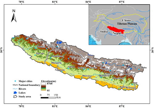
The study area is located in the central Himalayas, bordered by the Tibetan Plateau in the north and the Ganges Plain in the south (Figure 1). It spans 77°2′E to 88°58′N and 26°19′N to 31°29′N. It is about 1332 km long from east to west and 230 km long from north to south, with a total area of approximately 270,000 km². The central mountain ranges in the study area include the Siwalik Mountains, the Lower Himalayas, and the Greater Himalayas. Elevation varies from 60 to 8768 m amsl. The world’s major rivers originate here, such as the Ganges and the Tsangpo-Brahmaputra. The vast elevation range and complex terrain mean they experience a wide range of climates, from low elevation humid subtropical climate to subtropical highland climate (Peel et al. 2007). The precipitation regime is driven by the Indian monsoon in summer and the mid-latitude westerlies in winter, with over 80% of annual precipitation occurring between June and September (Bohner 2006). Moreover, there has recently been a significant warming and drying trend (Norris et al. 2020). The forests are roughly divided into subtropical montane evergreen broadleaf forests, montane warm temperate mixed coniferous forests, and montane cold temperate coniferous forests. It is home to over 40 million people with a fragile economic and environmental, high poverty rates and fast population growth. Local livelihood is sustained by various timber and non-timber forest resources and is highly dependent on forests (Gurung et al. 2021). Study area involves three countries, China, Nepal, and India, with 39 administrative units at the district level.

Figure 1. Topography map and location of the central Himalayas (the digital boundary of the GRB from (Nie et al. 2017) and Tibetan Plateau from (Zhang et al. 2021).

2.2. Data source and processing

This study collected and used a variety of datasets (Table 1). The data used included standard Level 1 Terrain-corrected (L1T) orthorectified surface reflectance images of the 1995–2018 Landsat TM/ETM+/OLI archived in the GEE. All Landsat surface reflectance images were atmospherically corrected by the United States Geological Survey (USGS) using the Landsat Ecosystem Disturbance Adaptive Processing System (LEDAPS) or Land Surface Reflectance Code (LaSRC) algorithms. All remote sensing image processing is performed at GEE. In addition, slope and aspect were calculated from Shuttle Radar Topography Mapping Mission (SRTM) data to reflect terrain changes better and detect forests growing on steep slopes.

Table 1. Datasets used in this study.

	Data	Abbreviation	Data sources	Spatial resolution	Time series
Datasets	Landsat	–	http://landsat.usgs.gov	30m	1995–2018
	MODIS land cover type collection	MCD12Q1	https://lpdaac.usgs.gov/products/mcd12q1v006/	500m	2001–2019
	Climate change initiative-land Cover	CCI-LC	https://www.esa-landcover-cci.org/	300m	1992–2015
	GlobaLand30	–	http://www.globeland30.com	30m	2000, 2010 and 2020
	Finer resolution observation and monitoring-global land cover	FROMGLC	http://data.ess.tsinghua.edu.cn/data/Simulation/	30m	2015 and 2017
Natural factors	Annual maximum temperature	MAT	https://www.climatologylab.org/terraclimate.html/	2.5 arc minutes	1995–2018
	Annual minimum temperature	MNT	https://www.climatologylab.org/terraclimate.html/	2.5 arc minutes	1995–2018
	Average annual precipitation	PRE	https://www.climatologylab.org/terraclimate.html/	2.5 arc minutes	1995–2018
	Palmer drought severity index	PDSI	https://www.climatologylab.org/terraclimate.html/	2.5 arc minutes	1995–2018
	Elevation	DEM	https://earthexplorer.usgs.gov/	30m	–
	Aspect	ASP	Calculated according to elevation	30m	–
Anthropogenic factors	Population density	POP	https://www.worldpop.org/	100m	2000, 2007 and 2018
	Distance to roads	RDD	https://www.openstreetmap.org Euclidean distance from nearest roads	–	2017
	Distance to residential areas	RAD	https://www.icimod.org/ Euclidean distance from nearest residential areas	–	2000
	Distance to rivers	RVD	https://www.icimod.org/ Euclidean distance (m) from nearest rivers	–	2000
	Forest management		https://zenodo.org/record/5879022	100m	2015

To construct a reliable database of samples, we proposed to automatically collect samples through four sets of land cover products for our annual 30 m forest probability classification. Concretely, the MODIS Land Cover Type collection (MCD12Q1) used data with a spatial resolution of 500 m from 2001 to 2019. This dataset employed the IGBP classification system, which included 17 types such as Evergreen Needleleaf Forests, Evergreen Broadleaf Forests, etc. Climate Change Initiative-Land Cover (CCI-LC) has a 300 m spatial resolution for products from 1993 to 2015. This dataset utilized the Food and Agriculture Organization’s Land Cover Classification System (LCCS), which includes 22 types such as Cropland rainfed, Herbaceous cover, Tree or shrub cover, etc. The Finer Resolution Observation and Monitoring-Global Land Cover (FROM-GLC) has two phases of 30 m spatial resolution products in 2015 and 2017. GlobeLand30 included three phases of 30 m spatial resolution classification products in 2000, 2010 and 2020. The aforementioned two datasets consist of 10 land cover types, including cropland, forest, grassland, etc. To minimize the raster misalignment between products caused by different boundaries, we used GlobeLand30 to unify the grid positions. Also, four sets were resampled to 30 m resolution and reclassified as forest and non-forest.

Here we selected five natural factors and four background variables related to anthropogenic activities to analyze factors influencing forest change based on geographic detector. Namely, annual maximum temperature (MAT), annual minimum temperature (MNT), annual precipitation (PRE), Palmer Drought Severity Index (PDSI), elevation (DEM), aspect (ASP), population density (POP), distance to roads (RDD), distance to residential areas (RAD), distance to rivers (RVD). DEM and ASP remained constant throughout the study period, while MAT, MNT, PRE and POP changed throughout the detection period, and RDD, RAD and RVD were the state quantities of the initial year. In addition, we calculated the percentage of forest management area using the newly derived forest management dataset for 2015 (forest management activities’ pixels divided by all forest pixels in a 1 km grid cell) and analyzed the forest disturbance and recovery area under different forest management class, such as naturally regenerating forest without any signs of management, naturally regenerating forest with signs of management and agroforestry.

2.3. Methods

2.3.1. Research procedure

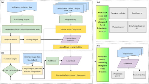
The research framework is divided into the following four main steps (Figure 2). First, the best pixel composite was applied in GEE to obtain Landsat surface reflectance images without cloud and shadow coverage (Zhu et al. 2015) for each year of the study area from 1995 to 2018. Annual forest probabilities were generated using a random forest classifier (Breiman 2001) based on a sample database obtained by statistical filtering. Second, applying the LandTrendr temporal segmentation algorithm (Kennedy et al. 2010) and calibration samples determined the forest disturbance and recovery. The overall accuracy and F1 score were calculated from the error matrix to evaluate the accuracy of the detection results. Third, the spatial and temporal evolution characteristics and country differences of forest disturbance and restoration were analyzed using methods such as the Theil-Sen estimator and stability analysis. Finally, we used the geographical detector (Wang et al. 2016) to evaluate the influence and interaction of natural and anthropogenic factors on the dynamics of Himalayan forests.

Figure 2. The flow chart to generate forest disturbance recovery mapping and influencing factors analysis, which includes (a) annual forest probability estimation module, (b) forest disturbance and recovery change mapping module, (c) forest spatial and temporal evolution analysis module and (d) analysis of factors influencing changes in forest dynamics module.

2.3.2. Image composition

High-quality satellite images are essential for generating annual forest maps. We used all available Landsat surface reflectance images during the from 1995 to 2018 to obtain as many good observations as possible. There are 13,931 scenes of Landsat 5/7/8 images in the study area, with an average of 17 good observations per year and poor observation quality in the high elevation region (Figure S1). In addition, considering that Landsat8/OLI has a higher sensor radiometric resolution than Landsat7/ETM+, we used the method of Roy et al. (2016) to improve the agreement between sensors, which generates normalized reflectance by cross-calibrating the different sensor reflectance. Subsequently, we used the pixel quality assessment bands to identify clouds, shadows, and snow/ice pixels for masked. These pixel quality assessments were generated using the FMASK algorithm (Zhu et al. 2015). Finally, the annual Landsat surface reflectance dataset for 1995–2018 was created using a centroid-based synthesis method (Flood 2013).

2.3.3. Training sample generation

This study extended an automatic method of generating and purifying high-quality samples. First, we performed an overlay analysis of four processed land cover products (MCD12Q1, CCI-LC, FROMGLC, and GlobeLand30) and developed a large initial sample database by creating numerous samples in stable forest regions (pixels with completely consistent types). Secondly, to minimize the spatial variation in the complex Himalayan landscape, we divided the study area into 324 hexagons with a 20 km side length. A total of 4214 samples were selected by random filtering within each grid to ensure spatial distribution and diversity of sample points. Thirdly, we applied pixel-based and neighborhood-based strategies to purify the samples to ensure reliability. Specifically, the pixel band values of the samples were extracted for the synthetic images of 1995, 2000, 2010, and 2018, respectively, and the outlier sample points were determined according to the 2-fold variance principle, which is based on a 95% confidence interval, which removes values that fall outside of the range of (μ-2σ, μ + 2σ). Then, we created sample kernels of size 3 × 3 Landsat pixels (∼0.81 ha) around the samples. The variance within each kernel was calculated and sorted in descending order, and sample points with variance in the top 10% of all four images were excluded. Finally, a total of about 6% of the samples were removed. 1746 and 2200 stable forest and non-forest samples were retained for subsequent classification.

2.3.4. Change reference sample

Obtaining consistent reference data in the Himalayan region is challenging. The availability of historical very high-resolution data varies with space and time. Therefore, we determined the forest disturbance and recovery labels by manual visual interpretation based on reference Google Earth history images supplemented with Landsat composite images within three detection periods. We obtained 372 and 314 forest disturbance and recovery samples in this study. More specifically, 124 disturbance and 107 recovery samples for 1995–2003; 133 disturbance and 102 recovery samples for 2004–2011; and 115 disturbance and 105 recovery samples for 2012–2018.

2.3.5. Random forests classification

Random Forests (RF) is a robust non-parametric machine learning algorithm that generates predictions by creating a set of regression trees from the bootstrap sampling of the original data and aggregating the results to improve prediction accuracy (Breiman 2001). RF has a clear advantage in multidimensional elemental data processing and is insensitive to overfitting, covariance problems, outliers and noise. It has been widely used for the supervised classification of long-term remote sensing data (Gómez et al. 2016).

In this study, we used the RF classifier to map the forest probabilities for each year. The number of trees was set to 500, the package fraction was 0.5, the variables split each time were equal to the square root of the number of predicted variables, and the minimum number of terminal nodes was set to 10. We randomly partitioned the aforementioned samples into a training set (90%) and a validation set (10%), Furthermore, considering the possible systematic differences in remote sensing images from different years, we trained images for each year from 1995 to 2018 using the same stable classes (i.e. forest and non-forest) to ensure comparable land cover classification results. Finally, we selected 12 variables as inputs to the RF classifier. These include six spectral bands: red, green, blue, near-infrared (NIR), shortwave infrared (SWIR1) and SWIR2. Four remote sensing indices: Normalized Difference Vegetation Index (NDVI), the Normalized Burn Ratio (NBR), modified Normalized Difference Water Index (mNDWI), green chlorophyll vegetation index (GCVI). and two topography-related bands: elevation and slope. For more detailed information on the input variables, see Supplementary Material S1.

2.3.6. Forest change detection

In this study, for each detection period, if the forest probability was less than 0.5 in both initial and final year classifications, the pixel was classified as permanent non-forest. Pixels with forest probability greater than 0.5 in either initial or final year were classified as forest. Since more than half of the study area (∼58%) is non-forest, some non-forest lands (Shrublands, fallow lands, etc.) have spectral characteristics close to forests and change under phenological or land use management practices influences, thus causing errors in forest change detection. Therefore, we masked out the permanent non-forest areas and performed forest change detection in the forested regions.

After establishing the annual forest classification probability stack, we applied the LandTrendr temporal segmentation algorithm to detect and characterize the change in class probability over time for each pixel. The main outputs of the model include the start and end times of the temporal segments, the segment lengths and the magnitude of the changes, etc. A more detailed description of this algorithm was previously provided by (Kennedy et al. 2010). In this study, the significance threshold (p = 0.05) and the maximum number of trajectory segments for the model fit were adjusted to 6 by referring to the fitting parameters of previous studies (Kennedy et al. 2018; Hu and Hu 2020). Besides, we divided the study period into three detection periods (1995–2003, 2004–2011, 2012–2018) for change detection to capture more detailed forest changes in the probability time series.

In this study, we conducted parameter tests on the magnitude of the change in classification probability, the year of change initiation, the year of change termination, the probability of change initiation classification, and the probability of change termination classification. In order to determine the optimal characteristic parameters of forest change in study area, we employed the calibration method of the optimal probability change magnitude (Yin et al. 2018). The F1 score for forest disturbance and recovery was calculated using the stable and change samples obtained in Section 2.3.3 as calibration samples with different combinations of feature discriminant parameters (for details, see S2, TableS2). The threshold of the relevant feature parameter corresponding to the F1 score reaching its maximum value is the optimal threshold. (1.) $$\begin{array}{c}F{1}_{\max }=\max \left\{2·\left(\frac{U{A}_i\times P{A}_i}{U{A}_i+P{A}_i}\right)\right\}\end{array}$$(1.) where UA is the user accuracy, PA is the producer accuracy, and i is the probability change step of 0.01.

To assess the accuracy of the forest change detection results, we performed forest change mapping validation every eight years using the stable forest samples, non-forest samples and forest change samples obtained above. In addition, the stable forest samples and stable non-forest samples are constant in each detection period, and there is only one category for a single pixel. Finally, the accuracy assessment of forest disturbance and recovery was performed by confusion matrix, including producer accuracy (PA), user accuracy (UA), overall accuracy (OA) and F1 score.

2.3.7. Statistical analysis

Theil-Sen slope estimate method was employed to detect time-series trends in Himalayan forest disturbance and recovery (Sen 1968). We first quantified the pixel areas of disturbance and recovery for each year and analyzed the entire research period and each detection period separately. The trend is calculated by: (2.) $$\begin{array}{c}\beta =\mathrm{Median}\left(\frac{x_j-x_i}{j-i}\right),1<j<i<m\end{array}$$(2.) where β is the Theil-Sen slope estimate. A positive value of β indicates an upward trend in a time series and vice versa; Median () is the median function; $x_j$ and $x_j$ denotes the forest disturbance or recovery in year j and i, respectively; m is the length of the forest change time series.

The coefficient of variation (CV) is a statistic that measures and evaluates the degree of variation of the observed values (Reed et al. 2002). Here the coefficient of variation was applied to assess the stability of forest disturbance and recovery. The CV is calculated as follows: (3.) $$\begin{array}{c}CV=\frac{\sqrt{\frac{\sum _{i=1}^n {\left(A_i-\overline{A}\right)}^2}{n-1}}}{\overline{A}}\end{array}$$(3.) where n is the total number of years; in this study, n equals 24. A_i is the forest change (disturbance or recovery) area in the ith year, and $\overline{A}$ is the average area from 1995 to 2018. The range of values for CV is between 0 and 1, with larger values indicating higher variability.

To capture the changes in national forests, we calculated the annual disturbance and recovery rates of forests in China, Nepal and India for each detection period, respectively. The calculation equations are as follows (Liu et al. 2023): (4.) $$\begin{array}{c}{R}_m\text{=}\frac{{\mathrm{a}}_{\text{im}}}{{\mathrm{A}}_{\mathrm{m}}}\mathrm{\times }100\text{\%}\end{array}$$(4.) where ${\mathrm{R}}_{\mathrm{m}}$ is the annual forest disturbance (recovery) rate in country m, ${\mathrm{A}}_{\mathrm{m}}$ is the total forest area of in country m during the detection period, and ${\mathrm{a}}_{\text{im}}$ is the forest disturbance (recovery) area in country m in the year i.

In addition, the intensity of absolute forest change (forest disturbance and recovery) was obtained for each country on the district-scale from 1995 to 2018. The expressions are as follows (Aldwaik and Pontius 2012): (5.) $$\begin{array}{c}CI=\frac{{\mathrm{C}}_{\mathrm{d}}+{\mathrm{C}}_{\mathrm{r}}}{{\mathrm{A}}_{\mathrm{f}}}\times \frac{1}{\mathrm{n}}\times 100\%\end{array}$$(5.) where CI is the intensity of forest change at the district level; ${\mathrm{C}}_{\mathrm{d}}$ and ${\mathrm{C}}_{\mathrm{r}}$ are the total amount of forest disturbance and recovery in a district during the study period, respectively; and ${\mathrm{A}}_{\mathrm{f}}$ is the total forest area at the beginning of detection period in a district; n is the total number of years.

2.3.8. Geographical detector

The geographic detector is a statistical tool that measures the spatial heterogeneity of geographic variables and explores potential influences. It consists of four modules, risk detector, factor detector, ecological detector and interaction detector. This method is usually more applicable than the linear model when there is a nonlinear relationship between the independent and dependent variables (Wang et al. 2016). In this study, factor detector was used to capture the effects of natural and anthropogenic factors on the changes in forest dynamics. The factor detector used the PD value to quantify the impact of the factor with the following mathematical expression: (6.) $$\begin{array}{c}PD=1-\frac{\sum _{h=1}^L N_h{\sigma }_h^2}{N{\sigma }^2}=1-\frac{\mathit{SSW}}{\mathit{SST}},\mathit{SSW}=\sum _{h=1}^L N_h{\sigma }_h^2,\mathit{SST}=N{\sigma }^2\end{array}$$(6.) where PD is the determining power of the influencing factor on forest change; the study region is divided into h to L sub-regions; $N_h$ and $N$ denote the number of units in strata h and the entire study region, respectively; ${\sigma }_h^2$ and ${\sigma }^2$ denote the variance of the dependent variable in strata h and the entire study region, respectively; SSW and SST are the sum of squares and the total sum of squares, respectively. PD values range from 0 to 1, meaning that the influencing factor explains PD $\times$100% of the dependent variable. The larger the PD implies that the influencing factor has a more substantial effect on forest change. In this study, a total of 6941 sample points with a resolution of 1 km were generated within the study area. Data processing was performed using the ‘GD’ package in the R programming language.

Using the interaction detector to identify interactions of influencing factors and determine whether the interaction between the two factors is weakening, enhancing, or completely independent of the effect on forest change. The interactive relationship was determined by comparing the PD values of individual factors and the two-factor interaction PD values, respectively (Table 2).

Table 2. Interaction categories of two factors and the interaction relationship.

Description	Interaction
$\mathrm{q}\mathrm{(}\text{X1}\mathrm{\cap }\text{X2}\mathrm{)}\mathrm{<}\text{ Min }\text{(q(}\text{X1}\mathrm{)}\text{,q}\mathrm{(}\text{X2}\mathrm{)}\mathrm{)}$	Nonlinear − weaken
$\mathrm{Min}(q(X1),q(X2))<q(X1\cap X2)<\mathrm{Max}(q(X1),q(X2))$	Univariate − weaken
$q(X1\cap X2)>\mathrm{Max}(q(X1),q(X2))$	Bivariate-enhance
$q(X1\cap X2)=q(X1)+q(X2)$	Independent
$q(X1\cap X2)>q(X1)+q(X2)$	Nonlinear − enhance

3. Results

3.1. Accuracy assessment of change detection

The forest disturbance and recovery aggregated map accuracy assessment in the study area from 1995 to 2018 showed an average OA of 0.92 ± 0.03 and a kappa coefficient of 0.89 ± 0.04. The F1 score was over 80% for all types, but the stability and change category errors differed between detection periods (Table 3). Overall, the average F1 score for the stable category is relatively higher than the change category. For each class, non-forest achieved the highest mean F1 score (0.96 ± 0.01), followed by stable forest (0.92 ± 0.04), forest recovery (0.87 ± 0.06), and forest disturbance (0.86 ± 0.03). The change detection results showed that forest disturbance and recovery were better captured. The average UA and PA of forest disturbance were 85.07% and 88.93%, respectively. The average UA of forest recovery was over 90%, but the lowest PA was 71.96%, mainly due to the confusion between the stable forest and the disturbance categories.

Table 3. Accuracy assessment of forest change detection for each period.

Period		1	2	3	4	UA	PA	F1	OA
1995–2003	1	228	4	5	0	96.20	96.20	96.20	89.11
	2	4	182	15	20	82.35	94.30	87.92
	3	4	4	102	10	85.00	82.26	83.61
	4	1	3	2	77	92.77	71.96	81.05
2004–2011	1	228	3	8	1	95.00	96.20	95.60	92.78
	2	4	182	1	9	92.86	94.30	93.57
	3	4	8	124	9	85.52	93.23	89.21
	4	1	0	0	83	98.81	81.37	89.25
2012–2018	1	230	1	3	0	98.29	97.05	97.66	94.78
	2	2	189	5	1	95.94	97.93	96.92
	3	4	3	105	12	84.68	91.30	87.87
	4	1	0	2	93	96.88	87.74	92.01

Note: 1: Non-forest; 2: Stable forest; 3: Forest disturbance; 4: Forest recovery; UA: User Accuracy; PA: Producer Accuracy; OA: overall accuracy. The F1 represents the harmonic mean of the PA and the UA.

3.2. Temporal evolution characteristics of transboundary forest disturbance-recovery

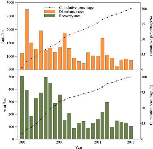
From 1995 to 2018, the total forest disturbance area in the study area was 2.94 × 10⁴ km², and the recovery area was 0.56 × 10⁴ km². In general, we found that 36% of the montane forests were disturbed, few areas undergoing forest recovery, and only 7% of the forests regenerated within 24 years. The average annual disturbed area for all three detection periods was greater than the recovered area (Figure 3). The maximum size of forest disturbance (0.27 × 10⁴ km²) occurred in 1996 and the minimum (0.06 × 10⁴ km²) in 2015. The top restoration area was 0.05 × 10⁴ km² in 1995. Notably, the size of forest disturbance from 1995 to 2003 accounted for about 46% of the total disturbed area. Both disturbed and restored areas showed a significant negative trend during the study period (Table S2), indicating a gradual decrease in transboundary forest change in the Himalayas. Yet the disturbance decreased more rapidly compared to the rate of change in recovery. In particular, the most significant rate of decline was observed from 2004 to 2011 (–60.01 km² yr⁻¹). However, the overall CV of forest recovery (0.56) outweighed that of disturbance (0.37), implying that transboundary forest recovery is less stable. Specifically, the most extensive CV for forest disturbance (0.33) and recovery (0.47) was in 1995–2003 and 2004–2011, respectively.

Figure 3. Annual forest disturbance-recovery area changes and cumulative percentage from 1995 to 2018.

3.3. Spatial evolution characteristics of transboundary forest disturbance-recovery

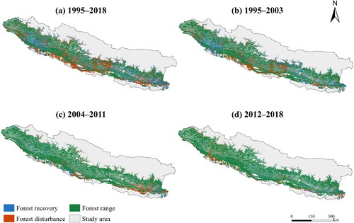
We found noticeable regional differences in transboundary forest change in the Himalayan region. In other words, disturbance and recovery occurred mainly in different zones. Most disturbances are in the southern Himalayan low elevation region and Gandaki Basin. In comparison, the restoration areas were distributed in the western part of the study area and the eastern part of Nepal (Figure 4). In addition, the spatial distribution of forest disturbance-restoration varied widely among the different detection periods. From 1995 to 2003, the spatial distribution of two types of forest change was similar to the distribution throughout the study period. Forest disturbance has been observed mainly in the Siwalik Hills and Terai region of the Himalayas and the Gandaki basin of Nepal. In contrast, forest recovery has occurred in the eastern part of the Uttaranchal state of India and the central-eastern part of the study area. From 2004 to 2011, although the distribution of forest disturbances was more concentrated, besides Siwalik and Terai in the southern part of the study area, where there were still persistent disturbances, the Koshi Basin in the eastern part of the study area showed a spreading trend from lower to higher elevations. Recovery areas were sporadically scattered across the study area. Forest disturbance within the eastern Middle Mountains of the study area decreased from 2012 to 2018, while Terai disturbance patches in India increased. Interestingly, the east part of the study area disturbed in 2004–2011 seemed to have shown forest regeneration after 2011.

Figure 4. Spatial patterns of transboundary forest disturbance-recovery in each detection period. (a) 1995–2018, (b) 1995–2003, (c) 2004–2011, (d) 2012–2018.

3.4. Analysis of national differences and intensity of transboundary forest change

3.4.1. Forest disturbance and recovery rates in China, India, and Nepal

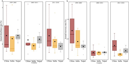
We further estimated China, Nepal and India’s forest disturbance and recovery rates for each detection period (Figure 5). Overall, Nepal experienced the highest forest disturbance rate (1.14%) and China had the highest forest recovery rate (0.29%) over the past 24 years. Characteristics of changes in forest disturbance and recovery rate were found in three countries. Although the forest disturbance rate was highest in Nepal from 1995 to 2003, it showed more pronounced volatility in China. India had the lowest disturbance rate (0.75%) among the three countries. The forest disturbance rate in Nepal had decreased from 2004 to 2011 and increased but reduced fluctuations in India. Furthermore, the forest disturbance rate in Nepal had been high until 2011, but the overall magnitude of change had been low. After 2011, China had the highest forest disturbance rate (1.18%). The recovery rate was relatively high in all countries before 2003. Specifically, China had the highest forest recovery rate (0.62%). India and Nepal exhibited similar overall levels of recovery rate, but forests within India were more unstable. It is noteworthy that the forest recovery rate was lower in the three countries from 2004 to 2011 compared to the other two detection periods. After 2011, China’s forest recovery rate rebounded, while India’s and Nepal’s recovery rates continue to decline.

Figure 5. Annual disturbance and recovery rates of forests in India, Nepal, and China for each detection period. (a) Forest disturbance rate; (b) forest recovery rate.

3.4.2. Spatial distribution of forest change intensity at the district level

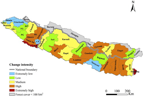
We used natural breakpoint method to classified district-level forest change intensity (CI) into five categories: extremely low (CI ≤ 1.44), low (1.44 < CI ≤ 1.63), medium (1.63 < CI ≤ 1.84), high (1.84 < CI ≤ 2.7), extremely high (CI ≥ 2.7) (Figure 6). Overall, the average annual change intensity on the district-scale was 1.86%, indicating that forest disturbance and recovery dynamics were relatively active from 1995to 2018. It is noticeable that Udham Singh Nagar (3.48%) and Darjiling (3.15%) were the only two regions in all districts where the CI exceeds 3%, which may be due to the lower elevation and more vulnerability to human activities (Chakraborty et al. 2017). About 45% of the forests (15 districts) had high and above CI. Still, only 33% (12 districts) of the forests had low and below CI, suggesting that the extent of forest change in the Central Himalayas has remained relatively high over the last 20 years. Moreover, the area disturbed was larger than the area recovered in each district, implying that forest disturbance was the main contribution to the variation of transboundary forest CI in the Himalayas.

Figure 6. Forest change intensity at the district level in the study area between 1995 and 2018. DD: Dehra dun; TG: Tehri Garhwal; RP: Rudra prayag; PG: Pauri Garhwal; BS: Bageshwar; CP: Champawat; UN: Udham Singh Nagar. The intensity of change (P) was divided into five categories: extremely low (p ≤ 1.44), low (1.44 < p ≤ 1.63), medium (1.63 < p ≤ 1.84), high (1.84 <p ≤ 2.7), extremely high (p ≥ 2.7).

3.5. Quantitative impact of influencing factors on forest dynamic change

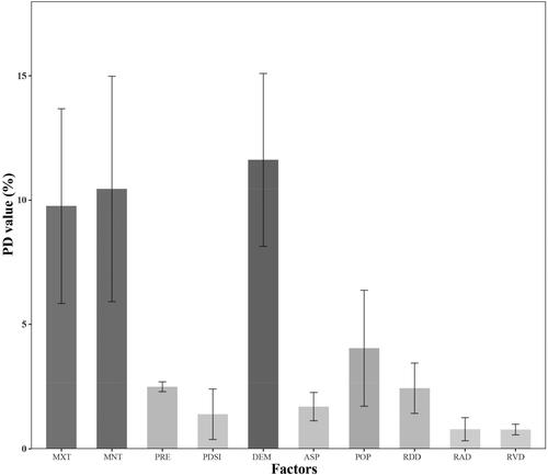
Factor detectors were applied to explain the degree of influence of each environmental factor on transboundary forest change. In this study, the PD values of natural and anthropogenic factors were determined by evaluating the impact of different factors on forest change. As shown in Figure 7, the impact of all the factors on forest change from 1995–2003 was ranked from highest to lowest: DEM > MNT > MXT > POP >PRE > RDD > ASP > PDSI > RAD > RVD. Of all the factors, the influence of natural factors was greater than that of anthropogenic factors. DEM was the most influential contributor (11.62%), followed by MNT (10.45%) and MXT (9.76%). This indicated that elevation and temperature were the dominant factors of forest change in the study area. With respect to anthropogenic factors, POP and RDD were the most contributing anthropogenic factors to forest change, with an average explanatory power of 4.04% and 2.43%, respectively. In general, elevation, temperature and population were the main determinants of the dynamics of the Central Himalayan forests.

Figure 7. PD values of the influencing factors from 1995 to 2018 in the transboundary forest. All PD values were statistically significant at the 1% level. The error bars represent the 1 – σ uncertainty. MXT: annual maximum temperature; MNT: annual minimum temperature; PRE: annual precipitation; DEM: elevation; ASP: aspect; POP: population density; RDD: distance to roads; RAD: distance to residential areas; RVD: distance to rivers.

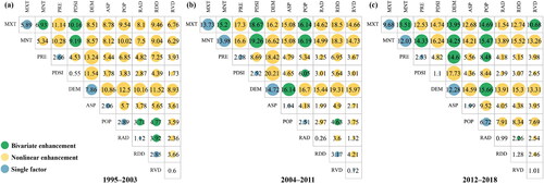
Interaction detection was employed to analyze whether the contribution of each factor to forest change between the two factors was enhanced or diminished or whether the effect was independent. Using an interaction detector, we identified interactions between nine influencing factors (Figure 8). The results showed that changes in transboundary forest dynamics were subject to synergistic enhancement effects among factors. Regardless of the detection period, the interaction PD value between any factors exceeded the PD value of a single. The types of interactions of the influencing factors were expressed as bivariate enhancement and nonlinear enhancement. Specifically, DEM, MNT and MXT interacted more strongly with other influencing factors, suggesting that elevation and temperature were the main factors affecting forest change. The nonlinear interaction between DEM and PRE was most substantial from 1995 to 2003. Interestingly, despite the limited explanatory power of PDSI for forest change, the interaction with factors such as temperature and elevation led to a substantial increase in explanatory power. Notably, the nonlinear interaction between PDSI and DEM had the greatest explanatory power (20.21%) on forest change from 2004 to 2011. Moreover, compared to before 2003, the proportion of anthropogenic-related interactions with higher explanatory power has gradually increased. POP had the strong bivariate interaction with DEM (15.66%), followed by RDD and MNT (15.52%), POP and MNT (15.47%) and RDD and DEM (15.30%) for the period 2012–2018. This indicated that the influence of anthropogenic activities continued to increase from 2003 onwards and became an important contribution to changes in transboundary forest dynamics.

Figure 8. Interaction effects of factors influencing transboundary forest dynamic change in each detection period. (a) 1995–2003; (b) 2004–2011; (c) 2012–2018; MXT: annual maximum temperature; MNT: annual minimum temperature; PRE: annual precipitation; DEM: elevation; ASP: aspect; POP: population density; RDD: distance to roads; RAD: distance to residential areas; RVD: distance to rivers.

4. Discussion

4.1. Transboundary forest disturbance and recovery mapping

Based on existing land cover data products and the GEE cloud platform, this study used machine learning and temporal segmentation to achieve dynamic mapping of transboundary forest disturbance and recovery in the Himalayas from 1995 to 2018. The results showed that the research framework enabled efficient quantitative and spatially explicit descriptions of forest disturbance and recovery. Numerous reliable land cover samples have always been a precondition for accurate land classification mapping. (Ghorbanian et al. 2020). In this study, we expanded a comprehensive sample collection method and constructed a stable and long-term reliable sample database, thus providing a basis for rapid implementation of high-precision mapping of Himalayan forest classification probabilities. In addition, previous studies have often used temporal segmentation algorithms for forest change detection based on one or more bands or spectral indices (Cohen et al. 2018). In contrast, we used the classification probability time series as the input to the LandTrendr algorithm. This approach can take interannual variability into account and effectively reduce the influence of external factors such as topography and atmosphere on surface reflectance (Wimberly et al. 2022). To our knowledge, this is the first implementation of this method in the Himalayan region while supporting the application of the framework of this study to identify other areas for forest change detection. Although we generated high-resolution (30 m) maps of forest disturbance and recovery in the central Himalayas, there are still some uncertainties.

High-quality remote sensing images are the basis for reliable disturbance and recovery detection. In the transboundary Himalayan mountains, the problems of enormous elevation differences, frequent cloud cover due to topographic rain, and the limited revisit period result in insufficient cloud-free clear images available throughout the year, which may affect the actual value of surface reflectance to some extent. Therefore, for the composition of annual images, unlike the existing studies that mostly used growing season period images (Liu et al. 2017; Senf et al. 2022). Here all available Landsat images for the study period were used. Nevertheless, there was still a lack of sufficient image composites in parts of the region in 1997. In addition, in order to minimize mixing spectral effects, we eliminated permanent non-forest areas and used a centroid-based image composition method before conducting disturbance and recovery detection. However, it is important to note that the exclusion of permanent non-forest areas based on a single date classification may inadvertently exemption forest pixels with lower probabilities in the initial and final years of observation.

Compared with the coarse spatial resolution images, this study adopted the fine spatial resolution Landsat images, which can capture the forest change processes at more fine scales. However, it is still difficult to identify the slow loss of vigor caused by insects in the forest and understory, as well as changes in individual tree stands. In addition, considering the diversity of forest types, short-rotation agricultural cropping patterns, and extensive smallholder economy characterize the Himalayas (Paudel et al. 2019; Wu et al. 2021). We divided the study period into three detection periods to enable a more comprehensive exploration and capture of forest disturbance and recovery. However, this study mapped the maximum forest change (disturbance and recovery) based on the pixel scale, which means that only one disturbance or recovery event per 900 m² was recorded during each detection period. This may lead to a certain degree of underestimation of change. In addition, pixel-based forest change detection mapping ‘salt and pepper’ noise is inevitable. A combination of object-oriented monitoring and temporal segmentation could be considered to reduce this effect.

The LandTrendr algorithm based on the GEE platform allowed the rapidly implementing large-scale forest change detection. However, it is critical to determine the optimal parameters of the algorithm to produce reliable detection results. In this study, the control parameters in the LandTrendr algorithm used the same parameters as in previous studies (Yin et al. 2018; Hu and Hu 2020). To determine the optimal magnitude of forest change, we performed an analysis of the feature combination parameters using a calibration sample. Moreover, reliable and accurate ground truth data are important for model calibration, but are often difficult to collect in the field. Calibration samples for this study were obtained based on 2 m spatial resolution Google Earth historical imagery in 2003, 2011 and 2018 and annual Landsat composite images to be visually interpreted. Nevertheless, the sparse availability of limited historical images and differences in the level of interpreters are still limitations of this study.

4.2. Spatio-temporal dynamics and influencing factors of transboundary forests

The transboundary forests of the Central Himalayas are undergoing remarkable changes. The study area generally suffered from continuous forest disturbance from 1995 to 2018, but recover with a gradually decreasing trend (Figure 3). The three detection periods found that more dramatic forest changes occurred in the study area until 2003, after which the magnitude of changes moderated. Similar situations have been found in other parts of the Himalayas (Paudel et al. 2016; Mannan et al. 2019). Meanwhile, this study resulted in a central Himalayan forest disturbance rate of 1.22%/yr, which is higher than that in the contiguous United States (1.09%/yr) (Masek et al. 2013), northern forests in Canada (0.43%/yr) (Wulder et al. 2020), and European forests (0.43%/yr) (Senf and Seidl 2020), similar to that in China (1.16%/yr) (Liu et al. 2023), but lower than the global average (5.6%/yr) (Hansen et al. 2013). While a previous study found a forest loss rate of 0.22% in the region (Gu et al. 2020). Our results are higher than this rate, which is unsurprising because it is well known that forest disturbance patterns can be naturally occurring or caused by human disturbance. In addition to agricultural expansion in the Himalayas, deforestation due to urbanization has permanently transformed the forest into another land cover type. There is also climate change, degradation of non-timber forest products such as firewood extraction for household consumption, and fodder extraction for livestock that reduces forest cover or quality (Nandy et al. 2011; Gurung et al. 2021). Recently, the forest canopy detection study in the Terai region of the Himalayas also found that the forest affected by disturbance was larger than the area of deforestation (Aryal et al. 2021), which supported the finding of this study.

We found that about 36% of the montane forest was disturbed. Most of the disturbances occurred in the lower elevation regions of the southern Himalayas and the Gandaki Basin(Figure 4). Similarly, published studies in the Chitwan district of the south part of the Gandaki basin found a decrease in forest canopy density of −7.95% since 1989 with most of the forest area decreasing (Panta et al. 2008). In addition, the National Forest Condition Survey released by the Government of Nepal in 2015 reported that Siwalik in the southern Himalayas had the highest forest disturbance incidence (Department of Forest Research and Survey 2015). These case studies are consistent with the findings of this study. Notably, we found that few areas were experiencing forest recovery, which may be attributed to the study area’s subsistence and semi-commercial farming practices. Families own the land and the prospects for ecological restoration are limited by repeated cultivation and illegal encroachment (Teegalapalli and Datta 2016).

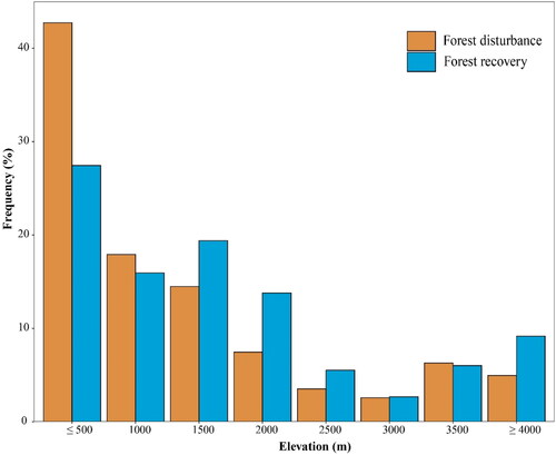
Understanding the influencing factors associated with forest disturbance and recovery is necessary to improve policies and mitigation measures for forest ecosystem management. In this study, we tried to quantitatively determine the attribution of forest change in terms of natural and anthropogenic factors. The results of the influence factor analysis indicated that natural factors play a key role in shaping forest disturbance and restoration in the Central Himalayas. The study area is the region with the most prominent elevation drop in the world (> 8000 above sea level). Climate and human activities have been governed by elevation as the most dominant factor in Himalayan forest change (Wu et al. 2021). Figure 9 clearly illustrates the heavy disturbances that occur at low elevations. Around 60% of the forest disturbance is below 1000 meters above sea level. Geographically, the region is hilly by nature, and forests in lower areas are more accessible to local communities and therefore suffer the most anthropogenic disturbance (Xie et al. 2021). Interestingly the high elevation forest seems to have recovered somewhat. Furthermore, the present results confirmed the importance of temperature on Himalayan forest changes, probably because the Himalayas is one of the fastest-warming regions in the world and the alpine biota is highly sensitive to climate warming. The combination of increased temperature and decreased precipitation results in temperature-induced drought stress in tropical mountains (Sigdel et al. 2018). Avalanche disturbance is an important process in many subalpine forest ecosystems, as it can damage or kill individual trees over areas larger than 10–100 hectares in fragile terrain environments (Bebi et al. 2009). Previous studies have also found that invasion and colonization by alien species can slowly reduce Central Himalayan forests’ growth and recovery potential (Shrestha et al. 2019). Besides, temperature and moisture are associated with wildfire, an important driver. Forests are vulnerable to irreversible degradation because of the positive feedback between vegetation and fire spread and intensity (Cochrane et al. 1999).

Figure 9. Occurrence frequency of transboundary forest disturbance and restoration along elevation gradient from 1995 to 2018 in the central Himalayas.

The analysis of interaction effects based on geographic detectors further emphasized that human factors have played an increasingly important role (Figure 8). In the central Himalayas, community forest management is a common livelihood strategy, with over 84.3% of forests affected by management activities. Forest change primarily occurs in naturally regenerating forests with signs of forest management (65.0%), followed by agroforestry (24.7%). However, forests without any signs of management, including primary forests, account for only 10.0% of the total. High population pressure and increased demand for agricultural land and timber harvesting have led to deforestation and degradation in the Himalayas. Population growth drives infrastructure development and road construction inevitably leads to increased forest fragmentation (Charlery et al. 2016). In addition, the expansion of illegal settlement agriculture in the Terai has contributed to forest disturbance and may result in the permanent conversion of forests to non-forest land uses. High elevation forests suffered degradation directly from stocking livestock units over nine times their carrying capacity (Chaudhary 2000). However, a quarter of the forests in Nepal are managed directly by the country’s rural population. Land use restrictions for forest management in these communities can limit agricultural production, logging and forest product extraction (Oldekop et al. 2019), thereby reducing forest disturbance and accelerating reforestation.

This study also found that all influence factor interactions were synergistic enhancement, implying that the effects of natural and anthropogenic factors on forest disturbance or recovery are not independent but synergistically enhanced. This is reasonable because past abundant studies also confirmed that the causes of changes in Himalayan forest dynamics are complex, with a high degree of connectivity among drivers. For example, international migration, transnational aid development programs, etc., significantly impact forest cover on a larger regional and national scale (Verma et al. 2021). The extensive interactions between disturbance agents may impact forest disturbance (Seidl et al. 2017). For example, interactions between drought and other controlling factors such as forest productivity, topography, fire weather, and management activities can affect fire intensity, severity, extent, and frequency (Littell et al. 2016). The formation of young forests after avalanches can affect the spread of wildfires by reducing landscape connectivity (Veblen et al. 1994). The Intergovernmental Panel on Climate Change (IPCC) has designated the Himalayan Hindu Kush as a data deficient region (IPCC 2014). It should be acknowledged that due to data and knowledge limitations, this study only provides a preliminary exploration of the influencing factors of forest changes in the central Himalayas. Future research is needed to conduct more detailed investigations of historical wildfires, avalanches, and other proxy indicators, to further explore multidimensional approaches for supplementing interactive studies, and to gain a more comprehensive understanding of the driving factors and mechanisms behind these dynamics.

Natural or human activities affect forest ecosystems’ structure, composition and function. The restoration or disturbance in forest ecosystems can positively or negatively impact ecosystem services, especially carbon storage (Bullock and Woodcock 2021). Changes in the type, magnitude, frequency, and intensity of disturbances can affect the balance between live and dead biomass stocks in forest ecosystems, leading to the potential for forests to become a carbon source or sink (Yatskov et al. 2019). It has also been confirmed that biodiversity nevertheless benefits from high severity disturbance events (Thom and Seidl 2016). In addition, the Himalayas is essentially a transboundary region, with considerable variation in forest disturbance and recovery among countries. Nepalese forests have generally higher disturbance, while China has high recovery rates but is more volatile (Figure 5). In view of the large disparities in geography, population, governance systems, level of economic development and culture of each country, the power allocated to the forest sector varies according to political boundaries. The future development of scientifically and effectively forest conservation policies and adaptation to changing disturbance regimes may be a key challenge for forest ecosystem management in each country.

5. Conclusions

This study combined supervised classification of machine learning model and time-series segmentation algorithms to identify disturbance and recovery of Himalayan transboundary forests from 1995 to 2018 using Landsat remote sensing image. Subsequently, the spatial and temporal evolution and national differences in forest disturbance-recovery and their influencing factors were investigated using trend and stability analysis as well as the geographical detector. This is the preliminary quantitative evaluation of patterns and trends in forest disturbance and recovery status in the Himalayan region. The results showed that forest disturbance was about five times greater than recovery over the past 24 years. We found that 36% of the montane forest was disturbed and only 7% of the forest regenerated. Forest disturbance and recovery showed a decreasing trend, but there was an apparent heterogeneity in the spatial pattern. Most disturbances occur in the lower elevation regions of the southern Himalayas and the Gandaki Basin. In contrast, the recovery areas were distributed in the western part of the study area and the eastern part of Nepal. In addition, annual disturbance rates and recovery rates of forests fluctuated markedly across countries during the study period. In particular, the highest disturbance rate was in Nepal (1.14%) and the highest recovery rate was in China (0.29%). The forest change intensity at an extremely high level was in Udham Singh Nagar district and Darjiling district. DEM, MXT, MNT and POP were the main influencing factors on the dynamics of transboundary forests in the Himalayas. The interaction of all factors showed synergistic enhancement, and RDD and DEM had the greatest explanatory power (19.31%). In addition, the expanded research framework of this study can serve as an important reference for forest change monitoring in other regions. These findings provided valuable information for data deficient regions and guidance for collaborative management of multinational forest ecosystems in the transboundary areas.

Data availability statement

The data that support the findings of this study are available from the corresponding author, upon reasonable request.

Disclosure statement

No potential conflict of interest was reported by the authors.

Additional information

Funding

This research was supported by the Second Tibetan Plateau Scientific Expedition and Research (Grant No. 2019QZKK0603), the Strategic Priority Research Program of the Chinese Academy of Sciences (Grant No. XDA20040201).

References

- Aldwaik SZ, Pontius RG. Jr., 2012. Intensity analysis to unify measurements of size and stationarity of land changes by interval, category, and transition. Landscape Urban Plann. 106(1):103–114. doi: 10.1016/j.landurbplan.2012.02.010.
- Allen CD, Breshears DD, Mcdowell NG. 2015. On underestimation of global vulnerability to tree mortality and forest die‐off from hotter drought in the anthropocene. Ecosphere. 6(8):art129. doi: 10.1890/ES15-00203.1.
- Aryal RR, Wespestad C, Kennedy R, Dilger J, Dyson K, Bullock E, Khanal N, Kono M, Poortinga A, Saah D, et al. 2021. Lessons learned while implementing a time-series approach to forest canopy disturbance detection in nepal. Remote Sensing. 13(14):2666. doi: 10.3390/rs13142666.
- Bański J, Janicki W. 2013. The influence of the eu’s eastern frontier on the socioeconomic situation of border areas. Eur Urban Reg Stud. 20(3):299–313. doi: 10.1177/0969776411432991.
- Bebi P, Kulakowski D, Rixen C. 2009. Snow avalanche disturbances in forest ecosystems—state of research and implications for management. For Ecol Manage. 257(9):1883–1892. doi: 10.1016/j.foreco.2009.01.050.
- Bohner J. 2006. General climatic controls and topoclimatic variations in central and high asia. Boreas. 35(2):279–295. doi: 10.1080/03009480500456073.
- Bowman DMJS, Kolden CA, Abatzoglou JT, Johnston FH, Van Der Werf GR, Flannigan M. 2020. Vegetation fires in the anthropocene. Nat Rev Earth Environ. 1(10):500–515. doi: 10.1038/s43017-020-0085-3.
- Boyd DS, Danson FM. 2005. Satellite remote sensing of forest resources: three decades of research development. Prog Phys Geogr. 29(1):1–26. doi: 10.1191/0309133305pp432ra.
- Breiman L. 2001. Random forests. Mach Learn. 45(1):5–32. doi: 10.1023/A:1010933404324.
- Bullock EL, Woodcock CE. 2021. Carbon loss and removal due to forest disturbance and regeneration in the amazon. Sci Total Environ. 764:142839. doi: 10.1016/j.scitotenv.2020.142839.
- Burrell AL, Sun Q, Baxter R, Kukavskaya EA, Zhila S, Shestakova T, Rogers BM, Kaduk J, Barrett K. 2022. Climate change, fire return intervals and the growing risk of permanent forest loss in boreal eurasia. Sci Total Environ. 831:154885. doi: 10.1016/j.scitotenv.2022.154885.
- Bustamante MMC, Roitman I, Aide TM, Alencar A, Anderson LO, Aragão L, Asner GP, Barlow J, Berenguer E, Chambers J, et al. 2016. Toward an integrated monitoring framework to assess the effects of tropical forest degradation and recovery on carbon stocks and biodiversity. Glob Chang Biol. 22(1):92–109., doi: 10.1111/gcb.13087.
- Chakraborty A, Ghosh A, Sachdeva K, Joshi PK. 2017. Characterizing fragmentation trends of the himalayan forests in the kumaon region of uttarakhand, india. Ecol Inf. 38:95–109. doi: 10.1016/j.ecoinf.2016.12.006.
- Charlery L, Nielsen MR, Meilby H, Smith-Hall C. 2016. Effects of new roads on environmental resource use in the central himalaya. Sustainability. 8(4):363. doi: 10.3390/su8040363.
- Chaudhary RP. 2000. Forest conservation and environmental management in nepal: a review. Biodiversity & Conservation. 9(9):1235–1260. doi: 10.1023/A:1008900216876.
- Chen C, Park T, Wang X, Piao S, Xu B, Chaturvedi RK, Fuchs R, Brovkin V, Ciais P, Fensholt R, et al. 2019. China and india lead in greening of the world through land-use management. Nat Sustain. 2(2):122–129., doi: 10.1038/s41893-019-0220-7.
- Cochrane MA, Alencar A, Schulze MD, Souza CM, Jr., Nepstad DC, Lefebvre P, Davidson EA. 1999. Positive feedbacks in the fire dynamic of closed canopy tropical forests. Science. 284(5421):1832–1835. doi: 10.1126/science.284.5421.1832.
- Cohen WB, Yang Z, Healey SP, Kennedy RE, Gorelick N. 2018. A landtrendr multispectral ensemble for forest disturbance detection. Remote Sens Environ. 205:131–140. doi: 10.1016/j.rse.2017.11.015.
- Cui B, Zhang Y, Wang Z, Gu C, Liu L, Wei B, Gong D, Rai MK. 2022. Ecological risk assessment of transboundary region based on land-cover change: a case study of gandaki river basin, himalayas. Land. 11(5):638. doi: 10.3390/land11050638.
- Da Cruz DC, Benayas JMR, Ferreira GC, Santos SR, Schwartz G. 2021. An overview of forest loss and restoration in the brazilian amazon. New For. 52(1):1–16. doi: 10.1007/s11056-020-09777-3.
- Department of Forest Research and Survey. 2015. State of Nepal’s Forests. Kathmandu: Department of Forest Research and Survey.
- Dhyani S, Dhyani D. 2020. Local socio-economic dynamics shaping Forest ecosystems in Central Himalayas. In: Roy N, Roychoudhury S, Nautiyal S, Agarwal S, Baksi S. editors. Socio-economic and eco-biological dimensions in resource use and conservation. Cham, CH: Springer; p. 31–60.
- Flood N. 2013. Seasonal composite landsat tm/etm + images using the medoid (a multi-dimensional median). Remote Sens. 5(12):6481–6500. doi: 10.3390/rs5126481.
- Ghorbanian A, Kakooei M, Amani M, Mahdavi S, Mohammadzadeh A, Hasanlou M. 2020. Improved land cover map of iran using sentinel imagery within google earth engine and a novel automatic workflow for land cover classification using migrated training samples. ISPRS J Photogramm Remote Sens. 167:276–288. doi: 10.1016/j.isprsjprs.2020.07.013.
- Gibson L, Lee TM, Koh LP, Brook BW, Gardner TA, Barlow J, Peres CA, Bradshaw CJA, Laurance WF, Lovejoy TE, et al. 2011. Primary forests are irreplaceable for sustaining tropical biodiversity. Nature. 478(7369):378–381. doi: 10.1038/nature10425.
- Gómez C, White JC, Wulder MA. 2016. Optical remotely sensed time series data for land cover classification: a review. ISPRS J Photogramm Remote Sens. 116:55–72. doi: 10.1016/j.isprsjprs.2016.03.008.
- Gorelick N, Hancher M, Dixon M, Ilyushchenko S, Thau D, Moore R. 2017. Google earth engine: planetary-scale geospatial analysis for everyone. Remote Sens Environ. 202:18–27. doi: 10.1016/j.rse.2017.06.031.
- Gu C, Zhao P, Chen Q, Li S, Li L, Liu L, Zhang Y. 2020. Forest cover change and the effectiveness of protected areas in the himalaya since 1998. Sustainability. 12(15):6123. doi: 10.3390/su12156123.
- Gurung LJ, Miller KK, Venn S, Bryan BA. 2021. Climate change adaptation for managing non-timber forest products in the nepalese himalaya. Sci Total Environ. 796:148853. doi: 10.1016/j.scitotenv.2021.148853.
- Hamunyela E, Brandt P, Shirima D, Do HTT, Herold M, Roman-Cuesta RM. 2020. Space-time detection of deforestation, forest degradation and regeneration in montane forests of eastern tanzania. Int J Appl Earth Obs Geoinf. 88:102063. doi: 10.1016/j.jag.2020.102063.
- Hansen MC, Potapov PV, Moore R, Hancher M, Turubanova SA, Tyukavina A, Thau D, Stehman SV, Goetz SJ, Loveland TR, et al. 2013. High-resolution global maps of 21st-century forest cover change. Science. 342(6160):850–853., doi: 10.1126/science.1244693.
- Hu Y, Hu Y. 2020. Detecting forest disturbance and recovery in primorsky krai, russia, using annual landsat time series and multi–source land cover products. Remote Sensing. 12(1):129. doi: 10.3390/rs12010129.
- Huang C, Goward SN, Masek JG, Thomas N, Zhu Z, Vogelmann JE. 2010. An automated approach for reconstructing recent forest disturbance history using dense landsat time series stacks. Remote Sens Environ. 114(1):183–198. doi: 10.1016/j.rse.2009.08.017.
- IPCC. 2014. Climate change 2014: impacts, adaptation, and vulnerability. New York (NY): Cambridge University Press Cambridge; 1132.
- Kennedy RE, Yang Z, Cohen WB. 2010. Detecting trends in forest disturbance and recovery using yearly landsat time series: 1. Landtrendr—temporal segmentation algorithms. Remote Sens Environ. 114(12):2897–2910. doi: 10.1016/j.rse.2010.07.008.
- Kennedy RE, Yang Z, Gorelick N, Braaten J, Cavalcante L, Cohen WB, Healey S. 2018. Implementation of the landtrendr algorithm on google earth engine. Remote Sens. 10(5):691. doi: 10.3390/rs10050691.
- Littell JS, Peterson DL, Riley KL, Liu Y, Luce CH. 2016. A review of the relationships between drought and forest fire in the United States. Glob Chang Biol. 22(7):2353–2369. doi: 10.1111/gcb.13275.
- Liu J, Rasul G. 2007. Climate change, the himalayan mountains, and ICIMOD. Sustain Moun Dev. 53:11–14.
- Liu Z, Wang WJ, Ballantyne A, He HS, Wang X, Liu S, Ciais P, Wimberly MC, Piao S, Yu K, et al. 2023. Forest disturbance decreased in china from 1986 to 2020 despite regional variations. Commun Earth Environ. 4(1):15. doi: 10.1038/s43247-023-00676-x.
- Liu S, Wei X, Li D, Lu D. 2017. Examining forest disturbance and recovery in the subtropical forest region of zhejiang province using landsat time-series data. Remote Sens. 9(5):479. doi: 10.3390/rs9050479.
- Liu J, Yong DL, Choi C-Y, Gibson L. 2020. Transboundary frontiers: an emerging priority for biodiversity conservation. Trends Ecol Evol. 35(8):679–690. doi: 10.1016/j.tree.2020.03.004.
- Mannan A, Liu J, Zhongke F, Khan TU, Saeed S, Mukete B, ChaoYong S, Yongxiang F, Ahmad A, Amir M, et al. 2019. Application of land-use/land cover changes in monitoring and projecting forest biomass carbon loss in pakistan. Global Ecol Conserv. 17:e00535. doi: 10.1016/j.gecco.2019.e00535.
- Masek JG, Goward SN, Kennedy RE, Cohen WB, Moisen GG, Schleeweis K, Huang C. 2013. United states forest disturbance trends observed using landsat time series. Ecosystems. 16(6):1087–1104. doi: 10.1007/s10021-013-9669-9.
- Matricardi E, Skole DL, Costa OB, Pedlowski MA, Samek JH, Miguel EP. 2020. Long-term forest degradation surpasses deforestation in the Brazilian amazon. Science. 369(6509):1378–1382. doi: 10.1126/science.abb3021.
- Milodowski DT, Mitchard ETA, Williams M. 2017. Forest loss maps from regional satellite monitoring systematically underestimate deforestation in two rapidly changing parts of the amazon. Environ Res Lett. 12(9):094003. doi: 10.1088/1748-9326/aa7e1e.
- Mittermeier RA, Turner WR, Larsen FW, Brooks TM, Gascon C. 2011. Global biodiversity conservation: the critical role of hotspots. In: Zachos FE, Habel JC, editors. Biodiversity hotspots. Berlin: Springer; 3–22.
- Nandy S, Kushwaha SPS, Dadhwal VK. 2011. Forest degradation assessment in the upper catchment of the river tons using remote sensing and GIS. Ecol Indic. 11(2):509–513. doi: 10.1016/j.ecolind.2010.07.006.
- Nie Y, Sheng Y, Liu Q, Liu L, Liu S, Zhang Y, Song C. 2017. A regional-scale assessment of himalayan glacial lake changes using satellite observations from 1990 to 2015. Remote Sens Environ. 189:1–13. doi: 10.1016/j.rse.2016.11.008.
- Norris J, Carvalho L, Jones C, Cannon F. 2020. Warming and drying over the central himalaya caused by an amplification of local mountain circulation. Npj Clim Atmos Sci. 3(1):1–11. doi: 10.1038/s41612-019-0105-5.
- Oldekop JA, Sims KRE, Karna BK, Whittingham MJ, Agrawal A. 2019. Reductions in deforestation and poverty from decentralized forest management in nepal. Nat Sustain. 2(5):421–428. doi: 10.1038/s41893-019-0277-3.
- Panta M, Kim K, Joshi C. 2008. Temporal mapping of deforestation and forest degradation in Nepal: applications to forest conservation. For Ecol Manage. 256(9):1587–1595. doi: 10.1016/j.foreco.2008.07.023.
- Paudel B, Zhang Y-L, Li S-C, Liu L-S, Wu X, Khanal NR. 2016. Review of studies on land use and land cover change in Nepal. J Mt Sci. 13(4):643–660. doi: 10.1007/s11629-015-3604-9.
- Paudel B, Zhang Y, Yan J, Rai R, Li L. 2019. Farmers’ perceptions of agricultural land use changes in Nepal and their major drivers. J Environ Manage. 235:432–441. doi: 10.1016/j.jenvman.2019.01.091.
- Peel MC, Finlayson BL, Mcmahon TA. 2007. Updated world map of the köppen-geiger climate classification. Hydrol Earth Syst Sci. 11(5):1633–1644. doi: 10.5194/hess-11-1633-2007.
- Rao KS, Pant R. 2001. Land use dynamics and landscape change pattern in a typical micro watershed in the mid elevation zone of central Himalaya, India. Agricult Ecosyst Environ. 86(2):113–124. doi: 10.1016/S0167-8809(00)00274-7.
- Reed GF, Lynn F, Meade BD. 2002. Use of coefficient of variation in assessing variability of quantitative assays. Clin Diagn Lab Immunol. 9(6):1235–1239. doi: 10.1128/cdli.9.6.1235-1239.2002.
- Roy DP, Kovalskyy V, Zhang HK, Vermote EF, Yan L, Kumar SS, Egorov A. 2016. Characterization of landsat-7 to landsat-8 reflective wavelength and normalized difference vegetation index continuity. Remote Sens Environ. 185:57–70. doi: 10.1016/j.rse.2015.12.024.
- Sahana M, Hong H, Sajjad H, Liu J, Zhu AX. 2018. Assessing deforestation susceptibility to forest ecosystem in Rudraprayag District, India using fragmentation approach and frequency ratio model. Sci Total Environ. 627:1264–1275. doi: 10.1016/j.scitotenv.2018.01.290.
- Seidl R, Thom D, Kautz M, Martin-Benito D, Peltoniemi M, Vacchiano G, Wild J, Ascoli D, Petr M, Honkaniemi J, et al. 2017. Forest disturbances under climate change. Nat Clim Chang. 7(6):395–402. doi: 10.1038/nclimate3303.
- Sen PK. 1968. Estimates of the regression coefficient based on Kendall’s tau. J Am Stat Assoc. 63(324):1379–1389. doi: 10.1080/01621459.1968.10480934.
- Senf C, Seidl R. 2020. Mapping the forest disturbance regimes of Europe. Nat Sustain. 4(1):63–70. doi: 10.1038/s41893-020-00609-y.
- Senf C, Seidl R, Poulter B., 2022. Post‐disturbance canopy recovery and the resilience of Europe’s forests. Global Ecol Biogeogr. 31(1):25–36. doi: 10.1111/geb.13406.
- Sharma M, Areendran G, Raj K, Sharma A, Joshi PK. 2016. Multitemporal analysis of forest fragmentation in Hindu Kush Himalaya—a case study from khangchendzonga biosphere reserve, Sikkim, India. Environ Monit Assess. 188(10):596. doi: 10.1007/s10661-016-5577-8.
- Shen J, Chen G, Hua J, Huang S, Ma J. 2022. Contrasting forest loss and gain patterns in subtropical china detected using an integrated Landtrendr and machine-learning method. Remote Sensing. 14(13):3238. doi: 10.3390/rs14133238.
- Shrestha BB, Shrestha UB, Sharma KP, Thapa-Parajuli RB, Devkota A, Siwakoti M. 2019. Community perception and prioritization of invasive alien plants in chitwan-annapurna landscape, Nepal. J Environ Manage. 229:38–47. doi: 10.1016/j.jenvman.2018.06.034.
- Sigdel SR, Wang Y, Camarero JJ, Zhu H, Liang E, Peñuelas J. 2018. Moisture‐mediated responsiveness of treeline shifts to global warming in the Himalayas. Glob Chang Biol. 24(11):5549–5559. doi: 10.1111/gcb.14428.
- Sloan S, Sayer JA. 2015. Forest resources assessment of 2015 shows positive global trends but forest loss and degradation persist in poor tropical countries. For Ecol Manage. 352:134–145. doi: 10.1016/j.foreco.2015.06.013.
- Teegalapalli K, Datta A. 2016. Field to a forest: patterns of forest recovery following shifting cultivation in the eastern Himalaya. For Ecol Manage. 364:173–182. doi: 10.1016/j.foreco.2016.01.006.
- Thom D, Seidl R. 2016. Natural disturbance impacts on ecosystem services and biodiversity in temperate and boreal forests. Biol Rev Camb Philos Soc. 91(3):760–781. doi: 10.1111/brv.12193.
- UNEP & FAO. 2020. The state of the world’s forests 2020. In: Andrea Perlis, editor. Forests, biodiversity and people. Rome. UNEP & FAO.
- Vancutsem C, Achard F, Pekel JF, Vieilledent G, Carboni S, Simonetti D, Gallego J, Aragao LEOC, Nasi R. 2021. Long-term (1990–2019) monitoring of forest cover changes in the humid tropics. Sci Adv. 7(10):eabe1603. doi: 10.1126/sciadv.abe1603.
- Veblen TT, Hadley KS, Nel EM, Kitzberger T, Reid M, Villalba R. 1994. Disturbance regime and disturbance interactions in a rocky mountain subalpine forest. J Ecol. 82(1):125–135. doi: 10.2307/2261392.
- Verbesselt J, Hyndman R, Zeileis A, Culvenor D. 2010. Phenological change detection while accounting for abrupt and gradual trends in satellite image time series. Remote Sens Environ. 114(12):2970–2980. doi: 10.1016/j.rse.2010.08.003.
- Verma A, Schmidt-Vogt D, De Alban JDT, Lim CL, Webb EL. 2021. Drivers and mechanisms of forest change in the Himalayas. Global Environ Change. 68:102244. doi: 10.1016/j.gloenvcha.2021.102244.
- Wang J, Zhang T, Fu B. 2016. A measure of spatial stratified heterogeneity. Ecol Indic. 67:250–256. doi: 10.1016/j.ecolind.2016.02.052.
- Wimberly MC, Dwomoh FK, Numata I, Mensah F, Amoako J, Nekorchuk DM, Mcmahon A. 2022. Historical trends of degradation, loss, and recovery in the tropical forest reserves of Ghana. Int J Digital Earth. 15(1):30–51. doi: 10.1080/17538947.2021.2012533.
- Wu X, Paudel B, Zhang Y, Liu L, Wang Z, Xie F, Gao J, Sun X. 2021. Vertical distribution changes in land cover between 1990 and 2015 within the Koshi river basin, central Himalayas. J Geogr Sci. 31(10):1419–1436. doi: 10.1007/s11442-021-1904-2.
- Wulder MA, Hermosilla T, White JC, Coops NC. 2020. Biomass status and dynamics over Canada’s forests: disentangling disturbed area from associated aboveground biomass consequences. Environ Res Lett. 15(9):094093. doi: 10.1088/1748-9326/ab8b11.
- Xie F, Wu X, Liu L, Zhang Y, Paudel B. 2021. Land use and land cover change within the koshi river basin of the central Himalayas since 1990. J Mt Sci. 18(1):159–177. doi: 10.1007/s11629-019-5944-3.
- Yatskov MA, Harmon ME, Barrett TM, Dobelbower KR. 2019. Carbon pools and biomass stores in the forests of coastal Alaska: uncertainty of estimates and impact of disturbance. For Ecol Manage. 434:303–317. doi: 10.1016/j.foreco.2018.12.014.
- Yin H, Pflugmacher D, Li A, Li Z, Hostert P. 2018. Land use and land cover change in inner mongolia-understanding the effects of china’s re-vegetation programs. Remote Sens Environ. 204:918–930. doi: 10.1016/j.rse.2017.08.030.
- Zhang Y, Li B, Liu L, Zheng D. 2021. Redetermine the region and boundaries of Tibetan plateau. Geograph Res. 40(6):1543–1553.
- Zhang Y, Wu X, Zheng D. 2020. Vertical differentiation of land cover in the central himalayas. J Geogr Sci. 30(6):969–987. doi: 10.1007/s11442-020-1765-0.
- Zhu L, Liu X, Wu L, Tang Y, Meng Y. 2019. Long-term monitoring of cropland change near Dongting Lake, china, using the Landtrendr algorithm with Landsat imagery. Remote Sens. 11(10):1234. doi: 10.3390/rs11101234.
- Zhu Z, Wang S, Woodcock CE. 2015. Improvement and expansion of the FMASK algorithm: cloud, cloud shadow, and snow detection for Landsats 4–7, 8, and sentinel 2 images. Remote Sens Environ. 159:269–277. doi: 10.1016/j.rse.2014.12.014.
- Zhu Z, Woodcock CE. 2014. Continuous change detection and classification of land cover using all available Landsat data. Remote Sens Environ. 144:152–171. doi: 10.1016/j.rse.2014.01.011.