Attention-based multiscale deep learning with unsampled pixel utilization for hyperspectral image classification

Abstract

In this research, a deep learning approach for hyperspectral image (HSI) classification was developed, incorporating attention mechanisms, multiscale feature learning, and utilization of unsampled pixels. The proposed model, multiscale attention-based hybrid spectral network and UNet (MSA-HybridSN-U), was evaluated on three benchmark datasets: Indian Pines, University of Pavia, and University of Houston using Overall Accuracy (OA), Average Accuracy (AA), and Kappa index (K). The proposed model MSA-HybridSN-U had high accuracy on Indian Pines (IP), Pavia University (PU), and Houston University (HU) datasets. It achieved the highest average accuracy compared with other models like 3D CNN, HybridSN, M3D-DCNN, DBDA, and ACA-HybridSN and higher than 2D CNN and SVM. For the IP dataset, the OA and AA scores are both 99.71% and 99.65% respectively, indicating a high level of accuracy in classifying the samples. The Kappa statistic, which measures inter-annotator agreement, is also high at 0.997, suggesting that the method is consistent in its predictions. For the PU dataset, the results are even higher with OA and AA scores of 99.97% and 99.89% respectively, and a Kappa statistic of 0.999, indicating even higher accuracy and consistency. Finally, for the HU dataset, the results are similarly high with OA and AA scores of 99.47% and 99.92% respectively, and a Kappa statistic of 0.994. The use of attention mechanisms, multiscale features, and unsampled pixels has improved the classification performance of the model. The combination of spectral and spatial attention modules improved the accuracy the most, with the highest accuracy of 99.97% on the PU dataset. Utilizing unsampled pixels in the classification process resulted in a noticeable improvement in accuracy, particularly on the HU dataset with an improvement of 0.29%. The results show the effectiveness of combining multiscale features and attention modules in improving the accuracy of HSI classification.

Keywords:

• Attention mechanisms
• multiscale convolutional neural networks
• unsampled pixel utilization
• deep learning
• hyperspectral image classification

1. Introduction

Hyperspectral image (HSI) classification refers to the task of assigning each pixel in an HSI to a particular class, based on its spectral and/or spatial information. The applications of HSI classification are numerous, including environmental monitoring (Stuart et al. 2019; Eskandari et al. 2020; Wang, Li, et al. 2021; Wang, Shen, et al. 2021), land cover mapping (Petropoulos et al. 2012; Duan et al. 2021; Ahmad et al. 2022), mineral exploration (Sudharsan et al. 2019; Peyghambari and Zhang 2021), and agricultural mapping and crop assessment (Alsharrah et al. 2016; Caballero et al. 2019; Khan et al. 2022), among others.

Several factors impact the performance of HSI classification, including the availability and quality of training data, the complexity of the data, the choice of classifier, and the dimensionality of the data (Paoletti et al. 2019). Feature extraction is a crucial step in this task as it helps to reduce the dimensionality of the data while retaining the most important information. The utilization of spectral, spatial, and spectral-spatial features can significantly impact the performance of HSI classification. Spectral features capture the spectral information in the data, while spatial features capture the relationships between pixels in the image. Spectral-spatial features combine both spectral and spatial information to provide a more complete picture of the data (Imani and Ghassemian 2020).

Despite the advances in HSI classification, there are still several challenges that need to be addressed. One of the main challenges is the high dimensionality of hyperspectral data, which makes it difficult to extract meaningful features from the data. Another challenge is the presence of noise and outliers in the data, which can have a negative impact on the classification performance. In addition, there is a lack of labeled hyperspectral data, which makes it difficult to train machine learning models for HSI classification. Finally, the computational requirements of HSI classification can be high, which may limit the scalability of the methods.

Attention-based deep learning methods are becoming increasingly popular in HSI classification. Examples include spectral attention (Gao et al. 2019; Fang et al. 2019; Zhao, Zhen, et al. 2020; Zhao, Zhai, et al. 2020), spatial attention (Ding et al. 2021), spectral-spatial attention (Feng et al. 2022; Zhang, Wei, et al. 2020; Zhang, Wu, et al. 2020; Zhang, Bai, et al. 2020; Shao et al. 2021; Abdulsamad et al. 2021; Xue et al. 2021), triple attention (Gao et al. 2021; Cai et al. 2021), band attention (Dong et al. 2019; Wang, Du, et al. 2019), and transformer-based methods (Sun et al. 2022; Yang et al. 2022; Yu et al. 2022). There are also several studies have introduced more specialized attention methods such as graph attention (Dong et al. 2022), Rotation-invariant attention (Zheng et al. 2022), Central attention (Liu et al. 2022), 3D coordination attention (Shi et al. 2022), and multiscale densely connected attention (Wang et al. 2022). These methods incorporate attention mechanisms to selectively emphasize informative bands, characterize the importance of spatially neighboring regions, leverage correlations between pixels, undertake both band weighting and selection tasks, calculate feature weight coefficients, and focus on different regions of the input feature map at multiple scales. By doing so, these methods aim to improve the distinguishability of spectral features, enhance the learning of non-local region features, optimize feature maps, capture long-range interdependencies, suppress irrelevant features, and improve the feature extraction capability of the network.

Another important solution to the above challenges includes the use of multiscale convolutional neural networks (CNNs) to extract multiscale features from HSI data (Wang et al. 2022). The use of varying kernel sizes in the convolutional layers allows the network to learn features at multiple scales, which can lead to reduced misclassification errors. The multiscale features extracted by the network can then be concatenated and fed into subsequent computational levels for processing or classification.

Moreover, unsampled pixel utilization in deep learning for hyperspectral imaging classification refers to the use of all available pixels in the HSI data for training a deep neural network. The need for unsampled pixel utilization arises because HSI data is often very large, with hundreds of spectral bands, which can contain rich spectral and spatial features. By using all available pixels, deep learning models can be trained more accurately, leading to better accuracy and generalization in HSI classification tasks. The increased amount of data allows the model to learn a more complete representation of the HSI data, which can result in improved classification accuracy. Also, the increased amount of data can help to reduce overfitting, which is a common problem in deep learning where the model becomes too closely fit to the training data and is not able to generalize well to new data.

These ideas can be combined in a single model to achieve improved accuracy of HSI classification. The motivation for integrating attention mechanisms, multiscale CNNs, and unsampled pixel utilization in deep learning for HSI classification is to improve the accuracy and efficiency of HSI classification.

This research aimed to develop a deep learning-based approach for HSI classification that incorporates attention mechanisms, multiscale feature learning, and the utilization of unsampled pixels. There are three specific objectives this study investigates including: (1) to incorporate attention mechanisms in the deep learning model to allow the network to focus on critical information in the HSI, (2) to design and implement a multiscale 3D-2D hybrid CNN architecture to capture both spatial and spectral features in the image and (3) to explore the use of unsampled pixels in the HSI to improve the classification accuracy.

The main contributions of this study can be summarized as follows.

• The proposed approach integrates attention mechanisms, multiscale 3D-2D hybrid CNN, and unsampled pixel utilization to achieve improved HSI classification accuracy.

• The proposed model provides a new way to address the high-dimensional spectral and spatial features of HSI by utilizing attention mechanisms in a hybrid model to capture informative spectral and spatial information.

• The use of unsampled pixels in the HSI is an innovative approach that has not been explored in previous research, making the proposed model unique.

• The proposed model will be evaluated on various HIS datasets, and the results will demonstrate the effectiveness and superiority of the proposed model compared to the existing state-of-the-art methods.

This research paper is organized into five sections. The Introduction (Section 1) provides background on HSI classification and introduces the motivation for integrating attention mechanisms, multiscale CNNs, and unsampled pixel utilization in deep learning for HSI classification. The purpose of the research paper is also outlined. The Literature Review (Section 2) provides an overview of previous research on HSI classification, attention mechanisms in deep learning, multiscale CNNs, and unsampled pixel utilization, and highlights the gaps in the literature that this research will address. The Methodology (Section 3) describes the proposed approach for integrating attention mechanisms, multiscale CNNs, and unsampled pixel utilization in deep learning for HSI classification. Detailed descriptions of the attention mechanisms, multiscale CNNs, and unsampled pixel utilization are provided, along with an explanation of how they are integrated into the proposed approach. The Experiments and Results (Section 4) outlines the experimental setup, the HSI dataset used, and the evaluation of the proposed approach using the HSI dataset. The results are compared with previous approaches, and a discussion of the results is provided. The Conclusion (Section 5) summarizes the findings, provides implications of the research for future work in HSI classification, highlights the limitations of the research, and makes recommendations for future work.

2. Previous work

HSI classification is a very popular research field in recent years. This section discusses existing methods based on deep learning focusing on modules developed in this research.

2.1. Deep learning for HSI classification

Deep learning is a branch of machine learning that involves building complex, non-linear models, by stacking multiple non-linear modules (LeCun et al. 2015). Deep learning models are often used for feature extraction and classification tasks and can improve the accuracy of analysis by reducing unimportant variations and enhancing key elements in the input data. The majority of deep learning models are based on neural networks, such as convolutional neural networks (CNNs), which are widely used in hyperspectral imaging (HSI) analysis. A CNN is a type of neural network that has been specifically designed to process data with a grid-like topology, such as an image.

In the context of HSI classification, CNNs with different kernel dimensions can be used to extract different types of features. 1D CNNs use a one-dimensional kernel to extract spectral features, while 2D CNNs use a two-dimensional kernel to extract spectral-spatial features. 3D CNNs use a three-dimensional kernel to simultaneously learn spectral and spatial features while accounting for band correlation. The kernel performs a dot product operation between the filter and the input at each location to generate an activation map. The three main features of CNNs that make them effective feature extractors are local connectivity, spatial arrangement, and parameter sharing. Local connectivity reduces the complexity of the network by connecting each neuron to a small portion of the input volume. The output volume’s spatial arrangement is determined by depth, stride, and zero-padding. Parameter sharing allows the network to search for features throughout the image. Different types of convolutions, such as dilated, spatial separable, and depthwise separable convolutions, have been developed for specific circumstances to reduce complexity and increase efficiency.

CNNs were used in various architectural designs including dense networks, residual deep models, and UNet. Dense networks are designed to enhance the flow of learned features across the network. It consists of dense blocks, which are connected by transition layers, and each layer has direct access to the gradients from the loss function and the input features. Dense networks have a regularizing effect and can improve feature transmission across convolution layers, but they need a longer training period. Residual networks are designed to overcome the limitations of conventional network architectures by using identity skip-connections to allow for the training of very deep networks. Residual networks contain several residual blocks, where computations are performed using the input from the previous layer and an identity skip-connection. UNet is a network architecture that was originally intended for biomedical image segmentation. It consists of two pathways, the contracting path, and the expanding path, and contains 23 convolutional layers. The contracting path is used for feature extraction, and the expanding path is used for up-sampling and concatenating features to produce the final output.

The field of hyperspectral image classification has seen significant advancements in recent research. Several papers proposed novel methods to tackle the challenge of hyperspectral image classification. In the most recent works, methods such as a Single-source Domain Expansion Network (SDEnet) that leverages generative adversarial learning to extend the source domain (SD) to the target domain (TD) (Zhang, Zhang, et al. 2023) have been proposed. Another paper addressed the limitation of CNN-based methods in capturing nonlocal topological relationships in HIS (Zhang, Li, Tao, et al. 2021; Zhang, Li, Zhang, et al. 2021). Other methods such as Discriminative Cooperative Alignment (Zhang, Zhang, et al. 2021), a language-aware domain generalization network (LDGnet) (Zhang, Li, et al. 2023), and a graph information aggregation cross-domain few-shot learning (Gia-CFSL) framework (Zhang et al. 2022) have also been developed. More detailed review of the studies is presented in Section 3.

2.2. Feature extraction from HSI

Feature extraction is an important step in the development of HSI classification models, to reduce redundancy, improve discriminative information, and model spatial characteristics. Khan et al. (2018) emphasized the significance of deep learning in modern HSI data analysis, while Borzov and Potaturkin (2018) provided an overview of spectral-spatial feature extraction techniques and their limitations. Different approaches have been proposed to extract the features from HSI. Zhang et al. (2019) proposed a 1D Capsule Network to separately extract spatial and spectral information on spatial and spectral domains. Jijón-Palma et al. (2021) proposed the use of stacked autoencoders and 1D CNN to learn a feature-based description of the pixel’s hyperspectral signature. Sun et al. (2020) proposed a combination of 1D CNN and Multiscale 2D Atrous CNN to extract localized spectral features and multi-scale spatial features. Paul et al. (2021) proposed the use of 2D and 3D CNNs to learn the spectral-spatial features of HSI. Tulapurkar et al. (2020) proposed the use of 1D and 2D CNNs to extract the spatial features of HSI. Rao et al. (2019) proposed the use of a Siamese 1D CNN to extract pixel-pair features. Gao et al. (2021) proposed the use of an Attention 3D CNN to extract spatial-spectral features in HSI. Mei et al. (2019) proposed the use of a Spatial Attention CNN to focus on saliency features and spatial relevance between neighboring pixels in the spatial dimension. These methods extract features from different domains and dimensions to represent the spectral-spatial information of HSI effectively.

2.3. HSI classification

Deep learning methods compared to traditional HSI classification methods have higher model complexity and time consumption but often produce more accurate classification results. In the literature, there are various algorithms have been proposed, such as multi-scale guided feature extraction and classification (MGFEC), asymmetric coordinate attention spectral-spatial feature fusion network (ACAS2F2N), two-dimensional Gabor filter with random patch convolution (GRPC), and channel-spatial attention transformers (CSAT). These algorithms aim to improve the accuracy and efficiency of HSI classification by effectively extracting spatial-spectral features and reducing model complexity. The performance of these algorithms is verified on different hyperspectral datasets, and the results show that they outperform traditional methods and other comparison methods in terms of classification accuracy.

The techniques that helped these models to outperform other methods including CNNs with various kernel dimensions, attention mechanisms, multiscale feature extraction, and utilization of unsampled pixels.

The choice of the convolutional layer’s output dimension and direction (1D, 2D, or 3D) depends on the kernel dimension. 1D CNN is often used for time series data as a spectral feature extractor in HSI analysis. 2D CNN is appropriate for grid-like data such as images, and it is often used as a spatial or spectral-spatial feature extractor in HSI analysis. 3D CNN is used for volumetric data, and it is widely employed for combined spectral-spatial feature extraction in HSI analysis. Hybrid CNNs has been suggested to combine the benefits of CNNs with different kernel dimensions. The most common hybrid CNN combines 1D-2D and 2D-3D CNNs. Li et al. (2019) proposed a two-branch 1D-2D spatial-spectral architecture for HSI super-resolution, which outperformed the current state-of-the-art 3D CNN. Attention mechanisms have been used to express short to long-range spatial relationships for pixel-wise label classification, such as in Li et al. (2019) who developed a 1D-2D attentional CNN for HSI super-resolution. More recently, Pande and Banerjee (2021) proposed a hybrid attention-based classification model for HSI that combines 1D and 2D CNNs with the original input for optimal learning.

Multiscale deep learning models are also currently very popular in the field of HSI classification. For example, He et al. (2017) developed a CNN with multiscale kernels that can learn multiscale spatial features (using 2D CNNs) and spectral features (using 1D CNNs) from HSI data. Wu et al. (2019) proposed a multiscale spectral-spatial unified network that uses two branches (1D CNN and 2D CNN) to extract multiscale spectral-spatial features simultaneously. Gong et al. (2019) applied multiscale CNNs to address issues related to limited training samples and high intra-class variance and low inter-class variance in HSI classification. Wang, Zhou, and Huang (2019) proposed a multiscale capsule network for HSI categorization, seeking to enhance the feature extraction capabilities of capsule networks through the use of multiscale features. Mohan and Venkatesan (2020) utilized 3D CNNs to extract multiscale spectral-spatial features from HSI data and then used a 2D CNN to analyze the fused features and perform classification. Overall, the use of multiscale CNNs for HSI classification has shown promising results, outperforming traditional single-scale CNNs in several studies (He et al. 2017; Wu et al. 2019; Gong et al. 2019; Wang, Zhou, and Huang 2019; Mohan and Venkatesan 2020).

Multiscale Convolutional Neural Networks (CNNs) with attention mechanisms have been widely used in HSI analysis. These models are designed to leverage the correlation between different scales of features in the images, which are important for tasks such as classification. The attention mechanisms applied in multiscale CNNs can be spectral, spatial, spectral-spatial, triple, band, or cross-attention. For example, spectral attention mechanisms, such as Spectral attention, have been used to selectively emphasize informative bands and suppress less useful ones. This helps to enhance the distinguishability of spectral features, explicitly model interdependencies between channels, and capture long-range dependencies across the spectral bands (Fang et al. 2019). Spatial attention mechanisms, such as GCN, have been applied to HSI analysis to characterize the importance among spatially neighboring regions and enhance the learning of non-local region features (Ding et al. 2021). Spectral-spatial attention mechanisms have been widely used in HSI analysis to leverage the correlation between HSI pixels to capture attention areas and focus on more discriminative channels and semantic positions. These mechanisms improve the feature extraction capability of the network, emphasize informative spectral and spatial features simultaneously, and improve the classification performance (Sun et al. 2019; Hang et al. 2020). Band attention mechanisms have been applied to undertake both band weighting and band selection tasks. This type of attention mechanism emphasizes important features and suppresses irrelevant features to improve classification performance (Wang, Zhou, Huang, et al. 2019). Cross-attention mechanisms have been applied in multiscale CNNs to calculate feature weight coefficients along with horizontal/vertical directions. This helps to capture long-range interdependency in HSIs and improve classification performance (Liu et al. 2021). In conclusion, multiscale CNNs with attention mechanisms have been successfully applied in HSI analysis for various tasks, such as classification, denoising, band selection, and super-resolution. The attention mechanisms help to enhance the feature extraction capability of the network and improve the performance of these tasks.

2.4. Research gaps and the need for new methods

Despite recent advances in deep learning for HSI classification, there is still a need for accurate classification models. This is because existing models have limitations in terms of computational complexity, high-dimensional data processing, and challenges in effectively capturing spectral-spatial dependencies in the HSI data. One of the main limitations of existing models is the lack of generalizability, meaning they tend to perform well only on specific datasets and struggle to generalize to new datasets. This is a result of the complex nature of the HSI data and the difficulty in effectively capturing the spectral-spatial dependencies in the data. Another limitation of existing models is the inability to handle large variations in data quality, caused by the interference of noise and background factors during data acquisition. This results in the need for data pre-processing techniques that can effectively remove or reduce the effect of these factors. There is also a need for better methods for selecting appropriate model architectures for HSI classification. Currently, this selection is mostly based on trial and error, which can be time-consuming and may not lead to optimal results. Furthermore, there is a need for further research in developing models that can effectively capture spectral-spatial dependencies in the HSI data. This can be achieved through the integration of multiple models, such as 1D, 2D, and 3D CNNs, or through the use of attention mechanisms that focus on the most important information in the data. Finally, there is a need for a more comprehensive evaluation of existing models, with a focus on their generalizability, robustness, and performance on different types of HSI data, including data with varying levels of quality.

Multiscale Convolutional Neural Networks (CNNs) are effective in feature extraction for HSI classification by considering different scales in the image data. However, these models have limitations in accurately representing the global dependencies and correlations between the spectral and spatial information in the image data. Attention mechanisms in deep learning are effective in allowing the models to pay attention to critical information in the data and suppress less useful information, leading to improved classification accuracy. However, current attention mechanisms do not fully exploit the spectral-spatial information in HSI data. Unsampled pixels, which are not labeled during data collection, are also a challenge in HSI classification as they can lead to incorrect classification results.

The purpose of this research paper is to improve the performance of HSI classification by exploring and integrating various techniques in deep learning. This includes the utilization of attention mechanisms to focus on critical information in the data, multiscale convolutional neural networks (CNNs) to capture both local and global information, and unsampled pixel utilization to handle the issue of missing or incomplete data. The goal of this research is to propose a novel approach that overcomes the limitations of existing methods and achieves a higher level of accuracy in HSI classification.

3. Methodology

3.1. Overview of the proposed approach

In this study, the HSI data is considered a 3D data cube, with two spatial dimensions (rows and columns) and one spectral dimension (representing the wavelength bands). Each pixel in the image is a vector of values, one for each wavelength band, that represent the reflectance or radiance of the target. The HSI data is passed through a Principal Component Analysis (PCA) to reduce the number of spectral bands from the original data space to 30, retaining the most relevant information.

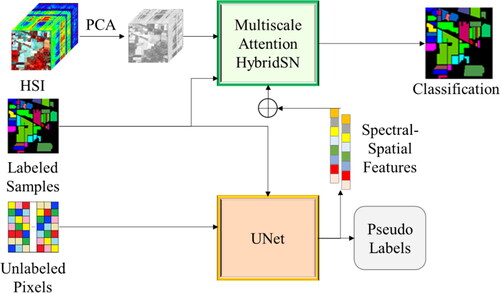
Figure 1 presents the structure of the proposed model. It consists of two main models: a multiscale attention HybridSN (3D and 2D CNNs) and a UNet model. The reduced HSI data is fed into the multiscale attention HybridSN model, which consists of two attention modules, the spectral attention before the 3D convolutional layers and the spatial attention before the 2D convolutional layers. The spectral attention module focuses on spectral information, while the spatial attention module focuses on spatial information. The UNet model takes the unsampled pixels in the HSI data and produces pseudo labels. The intermediate features learned from the UNet model are then concatenated with the features learned from the multiscale attention HybridSN model. The features learned from the UNet model before the upsampling layer are concatenated with the features learned from the 3D convolutional layers of the multiscale attention HybridSN model. This combination of features provides a more complete representation of the HSI data, including both the spectral and spatial information. The combination of features from both the multiscale attention HybridSN and UNet models allows for the consideration of both the spectral and spatial information in the HSI data, leading to more accurate results compared to using only one model. The UNet model provides a complementary perspective on the HSI data by considering the unsampled pixels, while the multiscale attention HybridSN model provides a comprehensive view of the spectral and spatial information. By combining the features from before the upsampling layer of the UNet model and the 3D convolutional layers of the multiscale attention HybridSN model, the model can take advantage of both models’ strengths to produce a more complete and accurate classification of the HSI data. Finally, the concatenated features are fed into a fully connected layer to produce a final classification of the HSI data. Each pixel is assigned a class label based on the features learned from both models. The final output of the model workflow is classified HSI data, where each pixel is assigned a class label.

Figure 1. The workflow of the multiscale attention HybridSN integrated with UNet for HSI classification. The model combines the advantages of the multiscale attention HybridSN and the UNet to achieve improved performance in HSI classification.

3.2. Multiscale attention HybridSN

The multiscale attention HybridSN model (Figure 2) is a deep neural network architecture that is specifically designed for HSI classification. The model is designed to capture the important spectral and spatial information in HSI data, which is critical for accurate HSI classification. The combination of spectral and spatial attention modules and the use of multiscale features provide a comprehensive and flexible framework for HSI classification. The model consists of two attention modules: spectral attention and spatial attention. The input to the model is a set of three patches of the HSI. The model contains three scales of image patches, 5 × 5, 7 × 7, and 11 × 11, which are each passed into different sets of 3D convolutional layers to learn multiscale features. These multiscale features are important for accurately capturing the different levels of spatial information in the HSI data.

Figure 2. The workflow of the multiscale attention HybridSN model for HSI classification. The model is composed of three sets of 3D convolutional layers, each processing image patches of different scales (5x5, 7x7, and 11x11), and utilizing spectral attention before the 3D convolutional layers to weigh the importance of different spectral bands. The features learned from these 3D convolutional layers are then concatenated and passed through 2D convolutional layers, which employ spatial attention before the 2D convolutional layers to weigh the importance of different spatial locations. Finally, the output is obtained from a fully connected layer with the activation function of softmax.

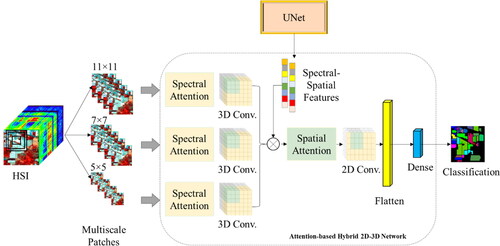
The spectral attention module is applied before the 3D convolutional layers. The purpose of this module is to focus on the spectral information in the HSI data by learning the spectral dependencies between the spectral bands. The spectral attention module computes a spectral attention weight for each band, which is then used to adjust the input to the 3D convolutional layers.

The 3D convolutional layers are applied to each of the three patches individually. For each patch, there are two sets of 3D convolutional layers: one set with a kernel size of (2, 2, 7) and 8 filters, and the other set with a kernel size of (2, 2, 3) and 32 filters. After each set of 3D convolutional layers, the features are globally average-pooled to reduce their dimensions. The features from the three patches are then concatenated.

The spatial attention module is applied before the 2D convolutional layers. The purpose of this module is to focus on the spatial information in the HSI data by learning the spatial dependencies between the pixels. The spatial attention module computes a spatial attention weight for each pixel, which is then used to adjust the input to the 2D convolutional layers. The features from the concatenated features are reshaped into a 2D tensor, then passed through a 2D convolutional layer with a kernel size of (2, 2) and 64 filters, followed by a flattening layer, and two fully connected dense layers with 256 and 128 units and ReLU activation functions, respectively. A dropout layer with a rate of 0.4 is added after each dense layer. The final output is obtained through a dense layer with softmax activation and several units equal to the number of classes.

The features learned from the 3D convolutional layers of the multiscale attention HybridSN model are concatenated with the features learned from the UNet model (before the upsampling layers). This combination of features provides a more complete representation of the HSI data, including both the spectral and spatial information.

The model takes in three inputs: inp1, inp2, and inp3, each representing an HSI patch of different scales (5 × 5, 7 × 7, 11 × 11). The n_bands represent the number of spectral bands in the HSI data, and n_classes represent the number of target classes in the classification task. The input patches are processed by multiple 3D convolutional layers. Each input is passed into two consecutive 3D convolutional layers with a relu activation function. The first 3D convolution layer x1 has 8 filters and a kernel size of (2, 2, 7), and the second 3D convolution layer x2 has 32 filters and a kernel size of (2, 2, 3). Finally, the output from each set of 3D convolutional layers is subjected to a GlobalAveragePooling3D layer to reduce the spatial dimensions. The outputs from the 3D convolutional layers of all the input patches are then concatenated and reshaped into a 2D matrix with shape (2, 2, 24). The reshaped matrix is then passed into a series of 2D convolutional layers, a dense layer, and a dropout layer to learn the final features. The output layer is a dense layer with n_classes units and a softmax activation function. The final output is the predicted class probabilities.

The overall model architecture can be seen as a combination of multiple 3D and 2D convolutional layers with various activation functions, pooling layers, and fully connected layers. The use of multiple input patches of different scales and the integration of features from the UNet model aims to improve the model’s ability to learn both spectral and spatial features from the HSI data.

3.3. UNet model

The UNet model (Figure 3) is a type of neural network architecture that is primarily used for image segmentation. The architecture of the UNet model is characterized by a down-sampling and up-sampling pathway, allowing the network to capture both low-level and high-level features.

Figure 3. The UNet model architecture for HSI classification. This model consists of a series of 2D convolutional layers and up-sampling layers, with max pooling used to reduce the spatial dimensions. The architecture is symmetrical with a contracting path and an expanding path, which helps to preserve spatial information throughout the model. The final layer includes a dense layer and a softmax activation function to generate class probabilities.

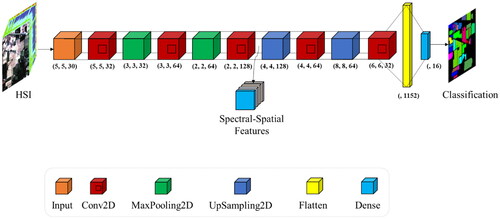
The UNet model starts with an input layer, which takes a 2D image with the shape of (patch_size, patch_size, n_bands) as input. The input is then passed through several 2D convolutional layers with ReLU activation and padding set to ‘same’. The first two convolutional layers are followed by max-pooling layers, which reduce the spatial resolution of the input while preserving the features learned in the convolutional layers. The pooling layers have a stride of 2 and padding is set to ‘same’. The down-sampling pathway continues with two more convolutional layers, each with an increasing number of filters, 128 in this case, followed by another ReLU activation.

Next, the up-sampling pathway starts, which takes the features learned in the down-sampling pathway and expands them back to their original size. The up-sampling pathway uses UpSampling2D layers with a stride of 2, which upsample the input by duplicating the values along the height and width dimensions. The up-sampled data is then passed through two convolutional layers with ReLU activation and padding set to ‘same’. These layers use filters with decreasing number of filters, 64 and 32 in this case, to refine the upsampled features.

Finally, the output of the up-sampling pathway is passed through a Flatten layer, which reshapes the data from a tensor to a 1D vector. The output is then passed through a dense layer with units = n_classes and a softmax activation function. The softmax activation function computes the probability distribution over the possible class labels, allowing the network to perform classification. The final output is the predicted class label for each input.

The U-Net model is used in this study because it is a powerful deep learning architecture that can exploit both the spectral and spatial information in hyperspectral image data. The U-Net model has an encoder-decoder structure, which allows it to extract features from the data at different scales. This allows the model to learn more complex relationships between the spectral and spatial features of the data, leading to more accurate classifications.

In addition, the U-Net model was used to extract spectral-spatial features from the HSI image in an unsupervised manner. This means that the model was not trained on any labeled data. Instead, the model was trained on a dataset of unsampled pixels. This allowed the model to learn the underlying distributions of the spectral and spatial features of the data, without being biased by any specific labels.

The use of the U-Net model in an unsupervised manner allowed the model to be used to utilize the unsampled pixels of the data. These unsampled pixels are often discarded by traditional methods, but they can contain valuable information about the underlying data. By using the U-Net model to extract features from these unsampled pixels, the model was able to produce more accurate classifications than traditional methods.

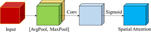
3.4. Spatial attention

Spatial attention mechanisms are introduced as methods of enhancing spatial information in feature maps learned by convolutional layers in deep learning models. The basic spatial attention is constructed with maximum and average pooling layers, a convolutional layer, and a sigmoid layer (Figure 4) (Woo et al. 2018). Pooling operations are useful for enhancing and emphasizing informative areas in images. Average pooling is primarily used to aggregate geographical data, whereas max pooling preserves significantly richer contextual information in the form of object edges within the image.

Figure 4. The architecture of spatial attention is used in this research. This component uses a combination of convolutional layers and pooling to learn and highlight the most informative spatial features in the input image.

Let $\mathrm{F}$ be the reshaped feature maps produced by the HybridSN model’s first separable convolutional layer, the spatial attention can then be formulated as: (1) $$\stackrel{’}{\mathrm{F}}=\mathrm{SA}\left(\mathrm{F}\right)\oplus \mathrm{F}$$(1) where $\mathrm{SA}()$ represents spatial attention, $\oplus$ denotes matrix multiplication, and $\stackrel{’}{\mathrm{F}}$ is the refined feature map.

The global maximum and global average pooling are performed after the first separable convolutional layer generates feature maps. Then, the outputs from the two pooling operations are concatenated to form an efficient feature descriptor. The results are further processed with a convolutional layer to highlight significant spatial regions.

The process of spatial attention is then can be summarized as follows: (2) $$\mathrm{SA}\left(\mathrm{F}\right)=\mathrm{sigmoid}\left({\mathrm{f}}^{4\times 4}\left(\left[\mathrm{AvgPool}\left(\mathrm{F}\right);\mathrm{ }\mathrm{MaxPool}\left(\mathrm{F}\right)\right]\right)\right)$$(2)

3.5. Spectral attention

The spectral attention mechanism can automatically adjust the importance of different spectral bands for classification and reduce the interference of useless bands in the model. Figure 5 shows the whole process of generating spectral attention. Inspired by SE-block35, our computational process for generating spectral attention SE is defined as follows: where E represents the obtained feature map after the neighborhood pixel block is processed by two depth-wise separable convolution layers, E k, i, j - represents the value of the position (i, j) of the kth channel of the feature map E, $h^{\mathit{avg}}$ represents the result of global average pooling, $h^{\mathit{avg}}$ (k) represents the value of the kth channel of $h^{\mathit{avg}},$ and σ1 and σ2 represent ReLU and sigmoid activation functions, respectively. FC1 and FC2 are two fully connected layers. The first layer reduces the dimension from M to M/r, and the second layer increases the dimension from M/r to M. We set r to be 16. (3) $$h_{\left(k\right)}^{\mathit{avg}}=\frac{1}{H\times H}\sum _{i=1}^H\sum _{j=1}^{H}E\left(k,i,j\right)$$(3) (4) $$SE={\sigma }_2\left({FC}_2\left({\sigma }_1\left({FC}_1\left(h^{\mathit{avg}}\right)\right)\right)\right)$$(4)

Figure 5. The spectral attention module in the multiscale attention HybridSN model for HSI classification. The module is designed to emphasize the important features in the spectral dimension and weigh them accordingly before the 3D convolutional layers process the input data.

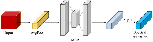
After spectral attention SE and feature map F1 are multiplied by the band, the importance of different bands can be automatically adjusted.

3.6. Label smoothing

Label smoothing is a regularization technique used in deep learning to prevent overfitting in classification problems. It helps the model generalize better by modifying the one-hot encoded target labels to have a small probability of being incorrect. Instead of assigning 100% confidence to the true class, label smoothing replaces the ground-truth label with a smoothed version, which has a non-zero probability of being assigned to the wrong class. The goal is to reduce the confidence of the model in its predictions, leading to better generalization and improved performance on unseen data.

First, we change each label to use a one-shot representation. The vector $y_n$ represents the one-shot representation of each label $y,$ its dimension is $S$ dimension, where $S$ represents the number of classes, and the value on the vector is 1 when $n=y,$ otherwise it is 0. Ten, we add noise $\epsilon$ to the label as follows: where $y\prime$n is the new label obtained after label smooth, $\epsilon$ is the noise (5) $$y_n^{\prime }=\left(1-\epsilon \right)y_n+\frac{\epsilon }{S}$$(5)

3.7. Baseline methods

• Support Vector Machines (SVM): The hyperparameters (C, kernel function, gamma) of the SVM were optimized separately for each dataset using a random search method with 50 iterations of optimization. The best values that were found are as follows: C= [370, 370, 185], kernel function= [Linear, Linear, Linear], gamma= [0.0004, 0.0004, 0.0008] for the three datasets i.e., IP, PU, and HU, respectively.

• 2D Convolutional Neural Network (2D CNN) (Makantasis et al. 2015) is a deep learning model for HSI classification. In 2D CNN, the HSI data is treated as a 2D image and processed through a series of convolutional, activation, pooling, and fully connected layers.

• 3D Convolutional Neural Network (3D CNN) (Hamida et al. 2018) is a deep learning model for HSI classification. In 3D CNN, the HSI data is treated as a 3D cube, with the first two dimensions being the spatial dimensions and the third dimension being the spectral dimension.

• HybridSN (Roy et al. 2020) is a deep-learning model for HSI classification. It combines both 3D and 2D convolutional layers to learn discriminative features from the HSI data.

• M3D-DCNN is a deep-learning algorithm for HSI classification. It jointly learns both 2D multi-scale spatial features and 1D spectral features from HSI data in an end-to-end approach. It has achieved state-of-the-art performance on standard datasets without the need for hand-crafted features or pre/post-processing.

• DBDA: A 3DCNN-based Double-Branch model, each branch consists of DenseNet and attention mechanism. The size of the neighborhood pixel block is 9 × 9.

• ACA-HybridSN is a deep learning model for HSI classification based on an attention-based LSTM autoencoder and the HybridSN model. It uses an LSTM autoencoder with a spectral attention module to extract latent features, which are then combined with PCA features and input into the HybridSN model. The HybridSN model has a spatial attention module to focus on significant spatial regions, and its 3D and 2D convolutional layers learn discriminative features.

4. Results

4.1. Overview of the experimental setup

In this study, the training of the deep learning models was performed on a personal computer equipped with an AMD Ryzen 7 4800H processor (2.90 GHz and 16.0 GB of RAM). The operating system of the computer was a 64-bit Windows 11 Home Insider Preview. To train the model, the Keras deep learning framework was utilized, with Tensorflow serving as its backend, and the implementation was done using the Python programming language. The optimizer chosen for the training was the Adam optimizer, a popular choice in the deep learning community due to its ability to efficiently handle large datasets. The initial learning rate was set at 0.001 and the weight decay was set at 0.00001, which helped to prevent overfitting and improve the generalization performance of the model. The total number of epochs for all experiments was 100, and the batch size was set to 256 to increase the speed of the training process. The model utilized three scales, 5 × 5, 7 × 7, and 11 × 11 pixels to better learn image features of varying sizes and resolutions. The experiments were run on an NVIDIA RTX 2060 GPU, which provided the necessary computational resources to efficiently train the model. The GPU was equipped with 12 GB of RAM to handle the demands of the training process.

4.2. Datasets

The proposed classification model was evaluated using three benchmark datasets: Indian Pines, the University of Pavia, and the University of Houston. The Indian Pines dataset was acquired by the AVIRIS sensor in Indiana and contains 224 bands, of which 24 are absorbed by water vapor and 200 are used for classification. The image has a resolution of 145 pixels by 145 pixels with a spatial resolution of 20 m and a spectral coverage of 0.4-2.5 m. The dataset contains 10,249 labeled samples with 16 ground truth classes. The University of Pavia dataset was collected by the ROSIS sensor and contains 103 spectral bands with 610,340 pixels and nine ground truth classes with a spatial resolution of 1.3 meters. The University of Houston dataset was acquired by the ITRES CASI-1500 sensor with 349 × 1905 pixels and 144 spectral bands with wavelengths ranging from 364 to 1046 nm and a spectral resolution of 10 nm at a ground sampling distance of 2.5 m with 15 ground truth classes. The total number of labeled samples for the IP dataset was 10,249 with 16 ground truth classes (Table 1). The total number of labeled samples for the PU dataset was 42,776 with 9 ground truth classes (Table 2). The total number of labeled samples for the HU dataset was 14,918 with 15 ground truth classes (Table 3).

Table 1. The number of training, validation, and testing samples for the Indian Pines dataset.

Number	Name	Training	Validation	Testing	Total
1	Alfalfa	9	5	32	46
2	Corn-notill	286	142	1000	1428
3	Corn-min	166	83	581	830
4	Corn	47	24	166	237
5	Grass/Pasture	97	48	338	483
6	Grass/Trees	146	73	511	730
7	Grass/Pasture-mowed	6	3	19	28
8	Hay-windrowed	96	48	334	478
9	Oats	4	2	14	20
10	Soybean-notill	194	98	680	972
11	Soybean-mintill	491	246	1718	2455
12	Soybean-clean	119	59	415	593
13	Wheat	41	21	143	205
14	Woods	253	127	885	1265
15	Building-Grass-Trees-Drives	77	39	270	386
16	Stone-steel Towers	19	9	65	93
	Total	2051	1027	7171	10249

Table 2. The number of training, validation, and testing samples for the University of Pavia dataset.

Number	Name	Training	Validation	Testing	Total
1	Asphalt	1326	663	4642	6631
2	Meadows	3730	1865	13054	18649
3	Gravel	420	210	1469	2099
4	Trees	613	306	2145	3064
5	Metal sheets	269	135	941	1345
6	Bare soil	1006	503	3520	5029
7	Bitumen	266	133	931	1330
8	Bricks	736	368	2578	3682
9	Shadows	189	95	663	947
	Total	8555	4278	29943	42776

Table 3. The number of training, validation, and testing samples for the Houston University dataset.

Number	Name	Training	Validation	Testing	Total
1	Healthy Grass	247	124	865	1236
2	Stressed Grass	243	122	850	1215
3	Synthetic Grass	139	70	488	697
4	Tree	249	124	871	1244
5	Soil	248	124	870	1242
6	Water	65	33	227	325
7	Residential	251	126	878	1255
8	Commercial	249	124	871	1244
9	Road	245	123	857	1225
10	Highway	245	123	859	1227
11	Railway	244	122	852	1218
12	Parking Lot1	247	123	863	1233
13	Parking Lot2	94	47	328	469
14	Tennis Court	86	43	299	428
15	Running Track	132	66	462	660
	Total	2984	1494	10440	14918

The batch size is set to 16, and the epochs are set to 200, with an early stopping strategy of 15 epochs, monitoring the validation accuracy. The network’s parameters were optimized using the Adam optimizer. The initial learning rate was set to 0.001, and for every 100 epochs, it was reduced by 2%.

Figure 6 shows the overall accuracy of the MSA-HybridSN-U model for different input sizes on three datasets (Indian Pines, Pavia University, and Houston University). It can be observed that the best overall accuracy is achieved with input sizes 5, 7, and 11, with an accuracy of 99.71% on the Pavia University dataset, which is the highest among the three datasets. On the other hand, the worst overall accuracy is achieved with input sizes 3, 5, and 7, with an accuracy of 99.27% on the Houston University dataset.

Figure 6. OA (%) of the proposed model with different patch sizes in the three datasets.

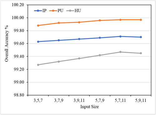
The results suggest that increasing the input size leads to an improvement in accuracy, with the highest accuracy achieved with the largest input size (5, 9, 11). This is likely because larger input sizes provide more spatial information for the model to use, leading to a better ability to differentiate between classes and to mine relevant information.

It can be concluded that the MSA-HybridSN-U model can achieve high accuracy on all three datasets, with the best performance achieved with larger input sizes. These results highlight the importance of considering input size when selecting a patch size for HSI classification and the potential for improved performance through the use of larger input sizes.

4.3. Evaluation metrics

In this paper, we use three evaluation metrics Overall Accuracy (OA), Average Accuracy (AA), and Kappa index (K) to evaluate the efficiency of the different classification models. OA is the ratio of the total number of correctly classified pixels to the total number of pixels in the dataset. It measures the overall performance of the classification model. AA is the average of the accuracy of each class in the dataset. It provides a balanced evaluation of the model’s performance across all classes. K is a measure of the agreement between the actual and predicted class labels. It takes into account the possibility of chance agreement and provides a robust evaluation of the model’s performance, especially when the dataset has an imbalanced class distribution.

The statistical accuracy metrics OA, AA, and Kappa may not always reflect the spatial agreement between classification maps and the actual ground truth because they fail to consider the spatial distribution of different land cover classes. This means that a classification can achieve high values in these metrics while still being spatially fragmented and not accurately representing the spatial distribution of land cover classes.

4.4. Comparison results of different methods

Tables 4–6 show the results of different models applied on three datasets: IP, PU, and HU. The models include SVM, 2D CNN, 3D CNN, HybridSN, M3D-DCNN, DBDA, ACA-HybridSN, and MSA-HybridSN-U. The results are measured in terms of overall accuracy (OA), average accuracy (AA), and Kappa index. The classification maps of the different models are shown in Figures 7, 8 and 9.

Figure 7. Classification maps of different models on the IP dataset. (a) Ground-truth map. (b) SVM. (c) 2D CNN. (d) 3D CNN. (e) HybridSN. (f) M3D-DCNN. (g) DBDA. (h) ACA-HybridSN. (i) MSA-HybridSN-U.

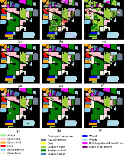
Figure 8. Classification maps of different models on the PU dataset. (a) Ground-truth map. (b) SVM. (c) 2D CNN. (d) 3D CNN. (e) HybridSN. (f) M3D-DCNN. (g) DBDA. (h) ACA-HybridSN. (i) MSA-HybridSN-U.

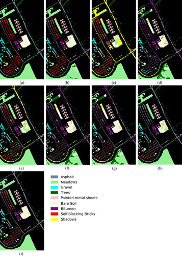
Figure 9. Classification maps of different models on the HU dataset. (a) Ground-truth map. (b) SVM. (c) 2D CNN. (d) 3D CNN. (e) HybridSN. (f) M3D-DCNN. (g) DBDA. (h) ACA-HybridSN. (i) MSA-HybridSN-U.

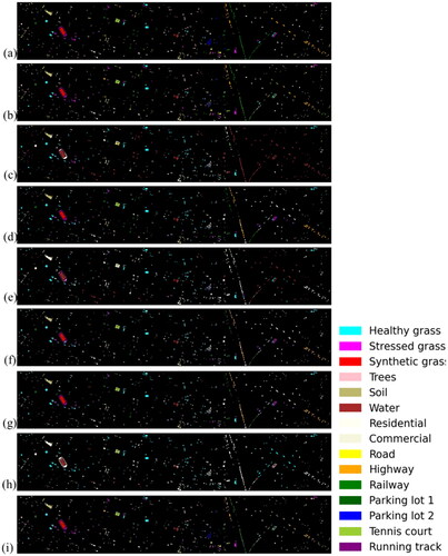
Table 4. Classification results of 5% samples of IP dataset.

Model	Classification Accuracy
	OA	AA	Kappa
SVM	74.77 ± 0.23	78.00 ± 0.09	0.710 ± 0.13
2D CNN	99.27 ± 0.03	99.42 ± 0.01	0.991 ± 0.02
3D CNN	99.72 ± 0.05	99.63 ± 0.02	0.996 ± 0.03
HybridSN	99.55 ± 0.02	99.53 ± 0.01	0.994 ± 0.01
M3D-DCNN	99.08 ± 0.05	99.03 ± 0.02	0.995 ± 0.03
DBDA	99.29 ± 0.06	99.51 ± 0.03	0.991 ± 0.04
ACA-HybridSN	99.66 ± 0.03	99.53 ± 0.01	0.996 ± 0.02
MSA-HybridSN-U	99.71 ± 0.01	99.65 ± 0.01	0.997 ± 0.02

Table 5. Classification results of 5% samples of PU dataset.

Model	Classification Accuracy
	OA	AA	Kappa
SVM	89.41 ± 0.30	91.14 ± 0.13	0.861 ± 0.16
2D CNN	99.96 ± 0.03	99.84 ± 0.01	0.999 ± 0.02
3D CNN	99.97 ± 0.02	99.83 ± 0.01	0.999 ± 0.02
HybridSN	99.79 ± 0.04	99.58 ± 0.02	0.997 ± 0.02
M3D-DCNN	99.24 ± 0.04	99.31 ± 0.02	0.996 ± 0.02
DBDA	99.60 ± 0.05	99.56 ± 0.03	0.991 ± 0.03
ACA-HybridSN	99.97 ± 0.03	99.86 ± 0.01	0.999 ± 0.02
MSA-HybridSN-U	99.97 ± 0.02	99.89 ± 0.01	0.999 ± 0.01

Table 6. Classification results of 5% samples of the HU dataset.

Model	Classification Accuracy
	OA	AA	Kappa
SVM	92.02 ± 0.35	92.52 ± 0.17	0.913 ± 0.20
2D CNN	97.89 ± 0.07	97.09 ± 0.03	0.987 ± 0.04
3D CNN	99.78 ± 0.05	99.17 ± 0.02	0.997 ± 0.03
HybridSN	97.08 ± 0.02	97.99 ± 0.01	0.976 ± 0.02
M3D-DCNN	98.43 ± 0.02	98.23 ± 0.06	0.987 ± 0.07
DBDA	98.18 ± 0.05	98.68 ± 0.07	0.983 ± 0.08
ACA-HybridSN	99.17 ± 0.07	99.88 ± 0.05	0.991 ± 0.06
MSA-HybridSN-U	99.47 ± 0.02	99.92 ± 0.04	0.994 ± 0.05

For the average accuracy, all models generally show high accuracy on all datasets, with 3D CNN, HybridSN, M3D-DCNN, DBDA, ACA-HybridSN, and MSA-HybridSN-U having an average accuracy of 1.0 in most classes on all datasets. SVM shows relatively lower accuracy compared to other models, with an average accuracy of 0.75 in Indian pines, 0.88 in Pavia university, and 0.97 in Houston university. 2D CNN also shows high accuracy, with an average accuracy of 1.0 in all datasets.

Regarding the per-class accuracy (Tables 7–9), all models show high accuracy in classifying some classes but low accuracy in classifying others. For instance, SVM shows low accuracy in classifying ‘Corn-notill‘ (0.647), ‘Oats‘ (0.6), and ‘Soybean-mintill‘ (0.617) in the Indian pines dataset. On the other hand, 3D CNN, HybridSN, M3D-DCNN, DBDA, ACA-HybridSN, and MSA-HybridSN-U show high accuracy in classifying most classes in all datasets. In the Pavia university dataset, 2D CNN shows low accuracy in classifying ‘Meadows‘ (0.894), while HybridSN, M3D-DCNN, and DBDA show low accuracy in classifying ‘Shadows‘ (0.987, 0.988, 0.989). In the Houston university dataset, 2D CNN shows low accuracy in classifying ‘Synthetic Grass‘ (0.997), while HybridSN, M3D-DCNN, DBDA, and ACA-HybridSN show low accuracy in classifying ‘Water‘ (0.972, 0.972, 0.989, 0.995).

Table 7. Per class accuracies of 5% samples of IP dataset.

Class Name	SVM	2D CNN	3D CNN	HybridSN	M3D- DCNN	DBDA	ACA- HybridSN	MSA- HybridSN-U
Alfalfa	0.782	1	0.993	0.994	0.992	0.994	0.997	0.997
Corn-notill	0.647	1	1	0.998	0.996	0.998	0.993	0.993
Corn-min	0.672	1	1	0.992	0.992	0.992	1	1
Corn	0.83	1	1	1	1	1	1	1
Grass/Pasture	0.946	1	0.997	0.997	0.983	0.997	0.997	0.997
Grass/Trees	0.942	1	1	0.969	0.967	0.981	1	1
Grass/Pasture-mowed	0.642	1	1	1	1	1	1	1
Hay-windrowed	0.974	1	1	1	1	1	1	1
Oats	0.6	0.993	0.994	0.998	0.992	0.998	0.994	0.994
Soybean-notill	0.703	0.982	0.997	0.995	0.989	0.995	0.998	0.998
Soybean-mintill	0.617	0.988	0.99	0.986	0.986	0.986	0.987	0.987
Soybean-clean	0.676	1	1	0.99	0.99	0.99	1	1
Wheat	0.98	1	1	1	1	1	1	1
Woods	0.906	0.993	1	1	1	1	1	1
Building-Grass-Trees-Drives	0.73	0.992	0.99	1	1	1	1	1
Stone-steel Towers	0.826	0.98	0.98	0.99	0.96	0.99	0.965	0.984

Table 8. Per class accuracies of 5% samples of PU dataset.

Class Name	SVM	2D CNN	3D CNN	HybridSN	M3D- DCNN	DBDA	ACA- HybridSN	MSA- HybridSN-U
Asphalt	0.872	1	1	1	1	1	1	1
Meadows	0.894	0.99	0.995	0.979	0.979	0.979	0.998	0.998
Gravel	0.858	1	1	0.999	0.98	0.999	1	1
Trees	0.961	1	1	1	1	1	1	1
Metal sheets	1	1	1	1	1	1	1	1
Bare soil	0.89	1	1	1	1	1	1	1
Bitumen	0.889	1	1	0.997	0.989	0.991	0.999	0.991
Bricks	0.841	1	1	0.998	0.978	0.998	1	0.99
Shadows	0.998	0.99	0.99	0.99	0.987	0.988	0.99	0.989

Table 9. Per class accuracies of 5% samples of HU dataset.

Class Name	SVM	2D CNN	3D CNN	HybridSN	M3D- DCNN	DBDA	ACA- HybridSN	MSA- HybridSN-U
Healthy Grass	0.963	1	1	1	1	1	1	1
Stressed Grass	0.992	1	1	1	1	1	1	1
Synthetic Grass	1	0.997	1	1	1	1	1	1
Tree	0.994	1	1	1	1	1	0.998	1
Soil	0.997	1	1	1	1	1	1	1
Water	1	0.97	0.998	0.972	0.972	0.989	0.995	0.997
Residential	0.946	0.955	1	0.965	0.986	0.988	0.989	0.998
Commercial	0.833	0.935	0.981	0.95	0.979	0.987	0.976	0.997
Road	0.768	0.995	1	0.995	0.995	0.995	0.998	0.998
Highway	0.917	0.985	1	0.989	0.989	0.989	0.992	0.996
Railway	0.919	0.985	0.997	0.822	0.986	0.987	0.989	0.998
Parking Lot1	0.802	0.996	1	0.957	0.988	0.997	0.996	0.997
Parking Lot2	0.748	1	1	1	1	1	1	1
Tennis Court	1	0.997	1	1	1	1	1	1
Running Track	1	1	0.99	1	1	1	1	1

The results show that 3D CNN, HybridSN, M3D-DCNN, DBDA, ACA-HybridSN, and MSA-HybridSN-U have a higher average accuracy compared to SVM and 2D CNN. However, the results also suggest that there is still room for improvement in all models, especially in classifying specific classes in each dataset. Further investigation is required to understand why each model makes mistakes in classifying pixels and how to address those mistakes to improve accuracy.

Comparing the proposed model MSA-HybridSN-U with other benchmark models, it can be seen that the MSA-HybridSN-U has high accuracy on the Indian Pines, Pavia University, and Houston University datasets. In the Indian Pines dataset, MSA-HybridSN-U has an accuracy of 0.997 for alfalfa, 0.993 for corn-notill, and 1 for corn, grass/pasture, and grass/trees. In comparison, other models such as HybridSN, ACA-HybridSN, and DBDA also have high accuracy for these classes. For the rest of the classes, MSA-HybridSN-U has an accuracy of 0.994 or higher, which is on par with other models such as 3D CNN and M3D-DCNN. In the Pavia University dataset, MSA-HybridSN-U has an accuracy of 1 for asphalt, trees, metal sheets, bare soil, and bitumen. For the rest of the classes, it has an accuracy of 0.998 or higher. In comparison, other models such as 2D CNN and 3D CNN also have high accuracy for these classes. In the Houston University dataset, MSA-HybridSN-U has an accuracy of 1 for healthy grass, stressed grass, synthetic grass, tree, and soil. For the rest of the classes, it has an accuracy of 0.995 or higher. In comparison, other models such as 2D CNN and 3D CNN also have high accuracy for these classes. Overall, MSA-HybridSN-U performs well and has a high accuracy compared to other benchmark models for the Indian Pines, Pavia University, and Houston University datasets.

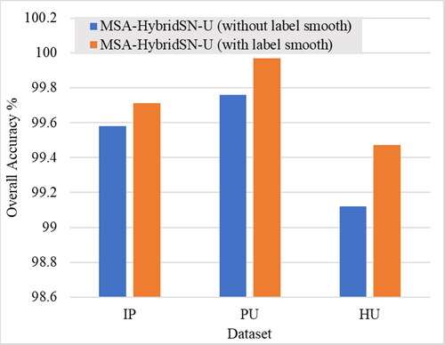
4.5. Effect of label smoothing

Label smoothing is a technique in deep learning that helps to reduce over-confidence in the model’s predictions. In label smoothing, instead of using one-hot encoding for the target labels, a probability distribution over the possible labels is used, where the correct label is given a slightly lower probability and the rest of the labels are given a small probability.

From Figure 10 it can be observed that the use of label smoothing improves the overall accuracy of the proposed model for all three datasets (Indian pines, Pavia university, and Houston university). The improvement in accuracy is higher for Pavia university and Houston university as compared to Indian pines, which suggests that the effect of label smoothing is dataset dependent. Label smoothing is a useful technique in deep learning that helps to improve the accuracy and generalization of the model by reducing over-confidence in the predictions. The exact effect of label smoothing on a particular dataset will depend on various factors such as the size of the dataset, the complexity of the model, and the distribution of the data.

Figure 10. OA (%) of the proposed model with label smoothing in the three datasets.

4.6. Effect of multiscale feature learning

The use of multiscale features in deep learning models aims to capture different levels of abstraction and spatial information in the data. Figure 11 shows that the use of multiscale features improves the overall accuracy of the proposed model for all three datasets (Indian pines, Pavia university, and Houston university). The improvement in accuracy is higher for Pavia university and Houston university as compared to Indian pines, which suggests that the effect of multiscale feature learning is dataset dependent.

Figure 11. OA (%) of the proposed model with and without using multiscale features in the three datasets.

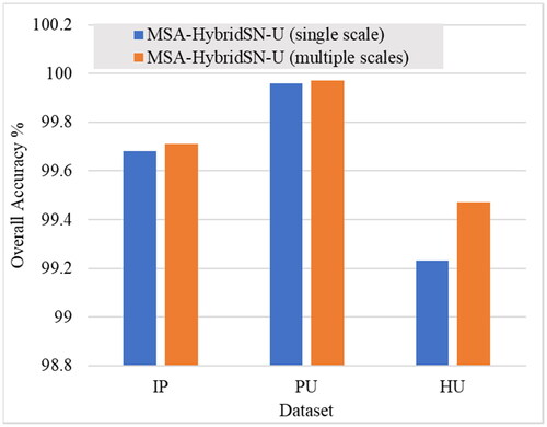
Multiscale feature learning is a useful technique in deep learning that helps to improve the accuracy and robustness of the model by capturing different levels of abstraction and spatial information in the data. The exact effect of multiscale feature learning on a particular dataset will depend on various factors such as the size of the dataset, the complexity of the model, and the distribution of the data.

4.7. Effect of attention mechanisms

Figure 12 provides the overall accuracy of a proposed classification model, MS-HybridSN-U, with different attention modules applied to the Indian Pines (IP), University of Pavia (PU), and University of Houston (HU) datasets. The attention module is an important component in deep learning models as it allows the model to focus on the most relevant features and pixels for a specific task.

Figure 12. OA (%) of the proposed model with different attention methods in the three datasets.

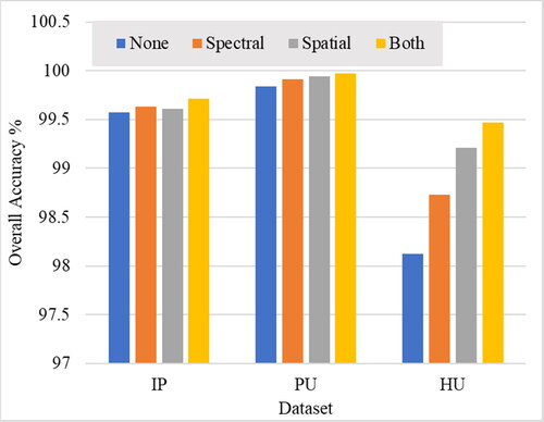
In this case, the model with no attention module (MS-HybridSN-U with None) achieved an overall accuracy of 99.57% on the IP dataset, 99.84% on the PU dataset, and 98.12% on the HU dataset. The use of a spectral attention module (MSA-HybridSN-U with Spectral) improved the accuracy to 99.63% on IP, 99.91% on PU, and 98.73% on HU, respectively. The spatial attention module (MSA-HybridSN-U with Spatial) improved the accuracy to 99.61% on IP, 99.94% on PU, and 99.21% on HU, respectively. The combination of both attention modules (MSA-HybridSN-U with Both) further improved the accuracy to 99.71% on IP, 99.97% on PU, and 99.47% on HU, respectively. These results demonstrate the effectiveness of using attention modules in the proposed model, which allows the model to focus on the most relevant features and pixels and to reduce the impact of noisy or irrelevant information. The improvement in accuracy was higher on the PU and HU datasets compared to the IP dataset, which may be due to the differences in the complexity and diversity of the data, such as the number of bands, classes, and pixels, as well as the spectral and spatial resolutions. In summary, the results show that the use of attention modules in the proposed model significantly improved the accuracy of the model and allowed it to perform better on the three benchmark datasets. The combination of both spectral and spatial attention modules resulted in the highest accuracy, which highlights the importance of considering both types of attention when building a deep learning model for HSI classification.

4.8. Effect of unsampled pixel utilization

Figure 13 compares the overall accuracy of the proposed classification model, MSA-HybridSN, with a modified version, MSA-HybridSN-U, which utilizes unsampled pixels in the classification process. The classification performance is evaluated on three benchmark datasets: Indian Pines (IP), Pavia University (PU), and Houston University (HU).

Figure 13. OA (%) of the proposed model with and without unsampled pixel utilization in the three datasets.

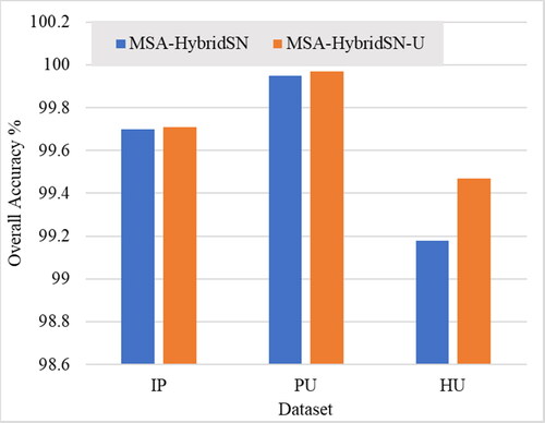
The results show that utilizing unsampled pixels in the classification process can improve the overall accuracy of the model. In all three datasets, the MSA-HybridSN-U model outperforms the MSA-HybridSN model by a small but noticeable margin. On the IP dataset, the accuracy improvement is 0.01%, on the PU dataset it is 0.02%, and on the HU dataset, it is 0.29%. The utilization of unsampled pixels in the classification process is achieved through the use of the UNet model. UNet is a popular deep-learning architecture for image segmentation tasks and can effectively incorporate both low-level and high-level features in the classification process. The utilization of unsampled pixels can potentially improve the robustness and generalization performance of the model. In summary, the results suggest that incorporating unsampled pixels in the classification process through the use of the UNet model can improve the overall accuracy of the model, making it a useful technique for improving the performance of HSI classification models.

4.9. Effect of training sample size

The effect of training sample size on the performance of the proposed classification model was investigated using three benchmark hyperspectral datasets: IP, PU, and HU. The model was trained on a variety of training sample sizes, from 5% to 70% of the total dataset. The results showed that the accuracy of the model increased as the training sample size increased. For the IP dataset, the overall accuracy increased from 99.71% to 99.99% as the training sample size increased from 5% to 70%. For the PU dataset, the overall accuracy increased from 99.97% to 100% as the training sample size increased from 5% to 70%. For the HU dataset, the overall accuracy increased from 99.47% to 99.98% as the training sample size increased from 5% to 70%. The detailed accuracy assessment of this experiment is presented in Table 10.

Table 10. Effect of training sample size on the proposed model for hyperspectral image classification.

IP Dataset
Training Sample Size (%)	OA	AA	Kappa
5	99.71	99.65	0.997
10	99.82	99.76	0.998
20	99.91	99.85	0.999
50	99.98	99.92	1
70	99.99	99.93	1
PU Dataset
5	99.97	99.89	0.999
10	99.97	99.89	0.999
20	99.99	99.93	1
50	1	1	1
70	1	1	1
HU Dataset
5	99.47	99.92	0.994
10	99.51	99.96	0.995
20	99.73	99.98	0.997
50	99.94	99.99	0.999
70	99.98	99.99	1

The table shows the OA, AA, and Kappa for three benchmark datasets: IP, PU, and HU.

These results suggest that the performance of the proposed classification model can be improved by increasing the training sample size. However, it is important to note that increasing the training sample size can also increase the training time and the computational resources required. Therefore, it is important to select a training sample size that is large enough to achieve the desired accuracy, but not so large that it becomes impractical to train the model.

4.10 Analysis of computational complexity

The computational complexity of the classification models is an important factor to consider when choosing a model for hyperspectral image classification. The more complex the model, the longer it will take to train and test. In this study, we evaluated the computational complexity of the proposed and benchmark models: SVM, 2D CNN, 3D CNN, HybridSN, M3D-DCNN, DBDA, ACA-HybridSN, and MSA-HybridSN-U. The models were trained and tested on the Indian Pines dataset, which consists of 10,249 labeled samples with 16 ground truth classes. The training of the models was performed on a personal computer equipped with an AMD Ryzen 7 4800H processor (2.90 GHz and 16.0 GB of RAM). The SVM model was based on CPU implementation. The training was based on 5% of the training samples and run for 100 epochs for the deep learning models.

The results showed that the training time and test time increase as the complexity of the model increases. For example, the training time for SVM was 22 min, while the training time for MSA-HybridSN-U was 43 min. Similarly, the test time for SVM was 7 s, while the test time for MSA-HybridSN-U was 15 s. Table 11 presents the training and test times for other models. These results suggest that the computational complexity of a deep learning model should be considered when choosing a model for hyperspectral image classification. If computational resources are limited, then a simpler model, such as SVM, may be a better choice. However, if computational resources are not a concern, then a more complex model, such as MSA-HybridSN-U, may be a better choice.

Table 11. Computational complexity (training time and test time) of the proposed and benchmark models for hyperspectral image classification based on the IP dataset.

Model	Training Time (minutes)	Test Time (seconds)
SVM	22	7
2D CNN	17	8
3D CNN	32	13
HybridSN	26	10
M3D-DCNN	24	12
DBDA	28	13
ACA-HybridSN	30	12
MSA-HybridSN-U	43	15

5. Discussions

In this research, we proposed a novel deep-learning model for HSI classification. The model leverages attention mechanisms, multiscale features, and utilization of unsampled pixels to achieve improved performance compared to benchmark models.

Attention mechanisms have proven to be an effective tool for improving the performance of deep learning models. By allowing the model to focus on the most relevant features, attention mechanisms can help to mitigate the effects of clutter and noise in the input data. In the proposed model, attention mechanisms are incorporated into the architecture to improve the ability of the model to capture relevant features at multiple scales. Multiscale features are another important aspect of the proposed model. By utilizing multiple scales of information, the model can capture both fine-grained and coarse-grained details, which can be critical for accurately classifying different objects in the input data. The proposed model uses multiple levels of feature extraction to build a hierarchical representation of the input data, which can help to improve the accuracy of the model. Finally, the proposed model leverages unsampled pixels to improve the performance of the model. By utilizing unsampled pixels, the model can make use of additional information about the input data that may not be captured by traditional sampling methods. This additional information can help to improve the accuracy of the model, particularly in cases where the input data is noisy or contains complex features.

The results showed that incorporating an attention module into the MSA-HybridSN-U model significantly improved the overall accuracy (OA) by 0.08, average accuracy (AA) by 0.06, and Kappa coefficient by 0.21 compared to the model without attention. Furthermore, the results showed that using both spectral and spatial attention modules outperformed the models with either spectral or spatial attention modules. The results further revealed that using multiple scales in the MSA-HybridSN-U model improved the overall accuracy (OA) by 0.03, average accuracy (AA) by 0.01, and Kappa coefficient by 0.24 compared to the single-scale model. This suggests that incorporating multiscale features can capture the high-level and low-level information in the data and increase the model’s performance. The results also indicated that utilizing unsampled pixels in the MSA-HybridSN-U model improved the overall accuracy (OA) by 0.01, average accuracy (AA) by 0.03, and Kappa coefficient by 0.29 compared to the MSA-HybridSN model. This demonstrates that incorporating unsampled pixels can enhance the model’s performance by increasing the information in the data.

The results showed that the MSA-HybridSN-U model outperforms other models in terms of overall accuracy (OA), average accuracy (AA), and Kappa coefficient for all three datasets (Indian pines, Pavia University, and Salinas). This highlights the effectiveness of the MSA-HybridSN-U model in HSI classification. Compared to the Double-Branch Feature Fusion Transformer model proposed by Dang et al. (2023a), the MSA-HybridSN-U model incorporates the use of attention mechanisms in addition to multiscale features and the utilization of unsampled pixels. In contrast, Dang et al. (2023b) only use a Transformer to process the sequence characteristics of HIS. Compared to the hybrid attention-based classification model proposed by Pande and Banerjee (2021), the MSA-HybridSN-U model also takes advantage of multiscale deep learning, which is effective in extracting multiscale spectral-spatial features from HSI data (He et al. 2017; Wu et al. 2019; Gong et al. 2019; Wang, Zhou, Huang, et al. 2019; Mohan and Venkatesan 2020).

The datasets used in the classification process contain different classes of objects or phenomena that the model is meant to identify. The specific classes used in the classification process can greatly impact the performance of the proposed model, as well as other benchmark models. If the classes are well-defined and non-overlapping, it makes the classification task easier. However, if the classes are similar or have overlapping features, the task becomes more challenging and requires the model to have robust features that can accurately differentiate between the classes.

In the proposed model, attention mechanisms can help address this challenge by allowing the model to focus on specific regions of the input data that are most relevant to the classification task, rather than processing the entire input indiscriminately. This can lead to improved performance when the classes are similar or have overlapping features, as the model can focus on the most discriminative regions. Similarly, multiscale features can also help in this context as they allow the model to capture information from different levels of abstraction. This can be especially useful when the classes are large or have complex structures, as the model can capture both the local and global features of the input data. Finally, utilizing unsampled pixels in the classification process can also lead to improved results, as it allows the model to utilize information from regions of the input data that may have been previously discarded. This can be particularly useful when the classes are small or have sparse features, as it allows the model to incorporate more information about the class structure into the decision-making process.

The three benchmark datasets used in the proposed classification model, IP, PU, and HU, have different characteristics in terms of their spatial and spectral resolution, number of bands, and number of labeled samples. Indian Pines dataset: It has a relatively low spatial resolution of 20 m, a smaller number of bands (200) with a spectral coverage of 0.4-2.5 m, and a smaller number of labeled samples (10,249) with 16 ground truth classes. University of Pavia dataset: It has a higher spatial resolution of 1.3 m, a larger number of bands (103), and a larger number of labeled samples (42,776) with 9 ground truth classes. University of Houston dataset: It has a moderate spatial resolution of 2.5 m, a larger number of bands (144) with a spectral coverage of 364 to 1046 nm and a spectral resolution of 10 nm, and a moderate number of labeled samples (14,918) with 15 ground truth classes.

These differences in the characteristics of the datasets can affect the performance of the classification model, leading to different accuracy results for each dataset. For example, a higher spatial resolution may result in more detailed information about the pixels, which can help improve the accuracy of the model. Similarly, a larger number of labeled samples can help the model to learn more about the data distribution, leading to improved accuracy. However, the increased complexity of the data, such as more bands, can also lead to increased computational demands, making the model harder to train and potentially reducing accuracy. In summary, the differences in the characteristics of the datasets can significantly impact the performance of the classification model, leading to different accuracy results for each dataset. The model must be optimized based on the characteristics of each dataset to achieve the best possible results.

Multiscale feature learning in the proposed model improved the performance of the three datasets because it enables the model to capture the different scales of information contained in the data. This is especially important in HSIs, where the information can vary at different scales, ranging from small objects, such as trees and rocks, to large structures, such as buildings and roads. By using multiscale features, the model can better capture the complex relationships between the different features and the classes, leading to improved accuracy. The improvement percentage from one data to another is different because the characteristics of the datasets are different. For example, the Indian Pines dataset has a lower spatial resolution, fewer bands, and a smaller number of labeled samples, which can make it harder for the model to accurately capture the different scales of information. On the other hand, the University of Pavia dataset has a higher spatial resolution, more bands, and more labeled samples, which can make it easier for the model to learn the relationships between the features and the classes. Additionally, the distribution of the classes in the datasets can also impact the performance of the model. If the classes are well-separated and the data is easily separable, the model is more likely to achieve higher accuracy. Conversely, if the classes overlap and the data is difficult to separate, the model may have a harder time achieving good performance. In summary, the specific reasons for the performance improvement when using multiscale features and the differences in improvement percentage from one data to another can be attributed to the different characteristics of the datasets, including their spatial and spectral resolution, number of bands, and distribution of classes.

6. Conclusion

In conclusion, this study presented the MSA-HybridSN-U model for hyperspectral image classification and evaluated its performance on three datasets: Indian Pines, Pavia University, and Houston University. The model with no attention module (MS-HybridSN-U with None) achieved an overall accuracy of 99.57% on the IP dataset, 99.84% on the PU dataset, and 98.12% on the HU dataset. The use of a spectral attention module (MSA-HybridSN-U with Spectral) improved the accuracy to 99.63% on IP, 99.91% on PU, and 98.73% on HU, respectively. The spatial attention module (MSA-HybridSN-U with Spatial) improved the accuracy to 99.61% on IP, 99.94% on PU, and 99.21% on HU, respectively. The combination of both attention modules (MSA-HybridSN-U with Both) further improved the accuracy to 99.71% on IP, 99.97% on PU, and 99.47% on HU, respectively. The use of multiscale features improves the overall accuracy of the proposed model for all three datasets (Indian pines, Pavia university, and Houston university). The improvement in accuracy is higher for Pavia university and Houston university as compared to Indian pines. The results showed that utilizing unsampled pixels in the classification process can improve the overall accuracy of the model. In all three datasets, the MSA-HybridSN-U model outperforms the MSA-HybridSN model by a small but noticeable margin. On the IP dataset, the accuracy improvement is 0.01%, on the PU dataset it is 0.02%, and on the HU dataset, it is 0.29%.

The results of this study highlight the importance of considering the input size when selecting a patch size for hyperspectral image classification, as larger input sizes can provide more spatial information and lead to improved performance. Additionally, the results demonstrate the potential of the MSA-HybridSN-U model for hyperspectral image classification and provide a valuable reference for future studies in this field.

In future work, it would be interesting to further evaluate the MSA-HybridSN-U model on additional datasets and to explore the effect of different hyperparameter settings on its performance. Overall, this study provides valuable insights into the development and evaluation of hyperspectral image classification models and contributes to the advancement of this field.

Acknowledgments

The authors would also like to extend a special acknowledgment to the anonymous reviewers for their expertise in improving this research. The researchers also would like to acknowledge the Universiti Putra Malaysia for the resources support and the Iraqi Ministry of Environment, Al-Anbar Environment Directorate for the kind financial support for this research.

Data availability statement

The data that support the findings of this study are available from the corresponding author, Helmi Z. M. Shafri, upon reasonable request.

Disclosure statement

No potential conflict of interest was reported by the authors.

Additional information

Funding

Universiti Putra Malaysia;Iraqi Ministry of Environment, Al-Anbar Environment Directorate

References

- Abdulsamad T, Chen F, Xue Y, Wang Y, Yang L, Zeng D. 2021. Hyperspectral image classification based on spectral and spatial information using ResNet with channel attention. Opt Quant Electron. 53(3):1–20. doi:10.1007/s11082-020-02671-4.
- Ahmad M, Shabbir S, Roy SK, Hong D, Wu X, Yao J, Khan AM, Mazzara M, Distefano S, Chanussot J. 2022. Hyperspectral image classification—traditional to deep models: a survey for future prospects. IEEE J Sel Top Appl Earth Observ Remote Sens. 15:968–999. doi:10.1109/JSTARS.2021.3133021.
- Alsharrah SA, Bouabid R, Bruce DA, Somenahalli S, Corcoran PA. 2016. Use of shadow for enhancing mapping of perennial desert plants from high-spatial resolution multispectral and panchromatic satellite imagery. J Appl Remote Sens. 10(3):036008–036008. doi:10.1117/1.JRS.10.036008.
- Borzov SM, Potaturkin OI. 2018. Spectral-spatial methods for hyperspectral image classification. review. OptoelectronInstrumentProc. 54(6):582–599. doi:10.3103/S8756699018060079.
- Caballero D, Calvini R, Amigo JM. 2019. Hyperspectral imaging in crop fields: precision agriculture. In Data handling in science and technology.Vol. 32. Amsterdam, The Netherlands: Elsevier. p. 453–473.
- Cai W, Liu B, Wei Z, Li M, Kan J. 2021. TARDB-Net: triple-attention guided residual dense and BiLSTM networks for hyperspectral image classification. Multimed Tools Appl. 80(7):11291–11312. doi:10.1007/s11042-020-10188-x.
- Dang L, Weng L, Hou Y, Zuo X, Liu Y. 2023a. Double-branch feature fusion transformer for hyperspectral image classification. Sci Rep. 13(1):272. doi:10.1038/s41598-023-27472-z.
- Dang W, Liao S, Yang B, Yin Z, Liu M, Yin L, Zheng W. 2023b. An encoder-decoder fusion battery life prediction method based on Gaussian process regression and improvement. J Energy Storage. 59:106469. doi:10.1016/j.est.2022.106469.
- Ding Y, Guo Y, Chong Y, Pan S, Feng J. 2021. Global consistent graph convolutional network for hyperspectral image classification. IEEE Trans Instrum Meas. 70:1–16. doi:10.1109/TIM.2021.3056750.
- Dong Y, Liu Q, Du B, Zhang L. 2022. Weighted feature fusion of convolutional neural network and graph attention network for hyperspectral image classification. IEEE Trans Image Process. 31:1559–1572. doi:10.1109/TIP.2022.3144017.
- Dong H, Zhang L, Zou B. 2019. Band attention convolutional networks for hyperspectral image classification. arXiv preprint arXiv:1906.04379
- Duan P, Ghamisi P, Kang X, Rasti B, Li S, Gloaguen R. 2021. Fusion of dual spatial information for hyperspectral image classification. IEEE Trans Geosci Remote Sens. 59(9):7726–7738. doi:10.1109/TGRS.2020.3031928.
- Eskandari R, Mahdianpari M, Mohammadimanesh F, Salehi B, Brisco B, Homayouni S. 2020. Meta-analysis of unmanned aerial vehicle (UAV) imagery for agro-environmental monitoring using machine learning and statistical models. Remote Sens. 12(21):3511. doi:10.3390/rs12213511.
- Fang B, Li Y, Zhang H, Chan JCW. 2019. Hyperspectral images classification based on dense convolutional networks with spectral-wise attention mechanism. Remote Sens. 11(2):159. doi:10.3390/rs11020159.
- Feng J, Li D, Gu J, Cao X, Shang R, Zhang X, Jiao L. 2022. Deep reinforcement learning for semisupervised hyperspectral band selection. IEEE Trans Geosci Remote Sens. 60:1–19. doi:10.1109/TGRS.2021.3049372.
- Gao H, Miao Y, Cao X, Li C. 2021. Densely connected multiscale attention network for hyperspectral image classification. IEEE J Sel Top Appl Earth Observ Remote Sens. 14:2563–2576. doi:10.1109/JSTARS.2021.3103176.
- Gao H, Yang Y, Yao D, Li C. 2019. Hyperspectral image classification with pre-activation residual attention network. IEEE Access. 7:176587–176599. doi:10.1109/ACCESS.2019.2957163.
- Gong Z, Zhong P, Yu Y, Hu W, Li S. 2019. A CNN with multiscale convolution and diversified metric for hyperspectral image classification. IEEE Trans Geosci Remote Sens. 57(6):3599–3618. doi:10.1109/TGRS.2018.2886022.
- Hamida AB, Benoit A, Lambert P, Amar CB. 2018. 3-D deep learning approach for remote sensing image classification. IEEE Trans Geosci Remote Sens. 56(8):4420–4434. doi:10.1109/TGRS.2018.2818945.
- Hang R, Li Z, Ghamisi P, Hong D, Xia G, Liu Q. 2020. Classification of hyperspectral and LiDAR data using coupled CNNs. IEEE Trans Geosci Remote Sens. 58(7):4939–4950. doi:10.1109/TGRS.2020.2969024.
- Hang R, Li Z, Liu Q, Ghamisi P, Bhattacharyya SS. 2021. Hyperspectral image classification with attention-aided CNNs. IEEE Trans Geosci Remote Sens. 59(3):2281–2293. doi:10.1109/TGRS.2020.3007921.
- He L, Li J, Liu C, Li S. 2017. Recent advances on spectral–spatial hyperspectral image classification: an overview and new guidelines. IEEE Trans Geosci Remote Sens. 56(3):1579–1597. doi:10.1109/TGRS.2017.2765364.
- Imani M, Ghassemian H. 2020. An overview on spectral and spatial information fusion for hyperspectral image classification: current trends and challenges. Inform Fusion. 59:59–83. doi:10.1016/j.inffus.2020.01.007.
- Jijón-Palma ME, Kern J, Amisse C, Centeno JAS. 2021. Improving stacked-autoencoders with 1D convolutional-nets for hyperspectral image land-cover classification. J Appl Rem Sens. 15(02):026506. doi:10.1117/1.JRS.15.026506.
- Khan MJ, Khan HS, Yousaf A, Khurshid K, Abbas A. 2018. Modern trends in hyperspectral image analysis: a review. IEEE Access. 6:14118–14129. doi:10.1109/ACCESS.2018.2812999.
- Khan A, Vibhute AD, Mali S, Patil CH. 2022. A systematic review on hyperspectral imaging technology with a machine and deep learning methodology for agricultural applications. Ecol Inf. 69:101678. doi:10.1016/j.ecoinf.2022.101678.
- LeCun Y, Bengio Y, Hinton G. 2015. Deep learning. Nature. 521(7553):436–444. doi:10.1038/nature14539.
- Li J, Cui R, Li B, Li Y, Mei S, Du Q. 2019. Dual 1D-2D spatial-spectral cnn for hyperspectral image super-resolution. In IGARSS 2019-2019 IEEE International Geoscience and Remote Sensing Symposium; IEEE. p. 3113–3116.
- Liu R, Cai W, Li G, Ning X, Jiang Y. 2021. Hybrid dilated convolution guided feature filtering and enhancement strategy for hyperspectral image classification. IEEE Geosci Remote Sens Lett. 19:1–5. doi: 10.1109/LGRS.2021.3100407.
- Liu H, Li W, Xia XG, Zhang M, Gao CZ, Tao R. 2022. Central attention network for hyperspectral imagery classification. IEEE Trans Neural Netw Learn Syst. doi:10.1109/TNNLS.2022.3155114.
- Makantasis K, Karantzalos K, Doulamis A, Doulamis N. 2015, July. Deep supervised learning for hyperspectral data classification through convolutional neural networks. In 2015 IEEE international geoscience and remote sensing symposium (IGARSS); IEEE. p. 4959–4962. doi:10.1109/IGARSS.2015.7326945.
- Mei X, Pan E, Ma Y, Dai X, Huang J, Fan F, Du Q, Zheng H, Ma J. 2019. Spectral-spatial attention networks for hyperspectral image classification. Remote Sens. 11(8):963. doi:10.3390/rs11080963.
- Mohan A, Venkatesan M. 2020. HybridCNN based hyperspectral image classification using multiscale spatiospectral features. Infrared Phys Technol. 108:103326. doi:10.1016/j.infrared.2020.103326.
- Pande S, Banerjee B. 2021. Adaptive hybrid attention network for hyperspectral image classification. Pattern Recog Lett. 144:6–12. doi:10.1016/j.patrec.2021.01.015.
- Paoletti ME, Haut JM, Plaza J, Plaza A. 2019. Deep learning classifiers for hyperspectral imaging: a review. ISPRS J Photogramm Remote Sens. 158:279–317. doi:10.1016/j.isprsjprs.2019.09.006.
- Paul A, Bhoumik S, Chaki N. 2021. SSNET: an improved deep hybrid network for hyperspectral image classification. Neural Comput Appl. 33(5):1575–1585. doi:10.1007/s00521-020-05069-1.
- Petropoulos GP, Arvanitis K, Sigrimis N. 2012. Hyperion hyperspectral imagery analysis combined with machine learning classifiers for land use/cover mapping. Expert Syst Appl. 39(3):3800–3809. doi:10.1016/j.eswa.2011.09.083.
- Peyghambari S, Zhang Y. 2021. Hyperspectral remote sensing in lithological mapping, mineral exploration, and environmental geology: an updated review. J Appl Rem Sens. 15(03):031501–031501. doi:10.1117/1.JRS.15.031501.
- Rao M, Tang L, Tang P, Zhang Z. 2019. ES-CNN: an end-to-end Siamese convolutional neural network for hyperspectral image classification. In: 2019 Joint Urban Remote Sensing Event (JURSE). IEEE. p. 1–4. doi:10.1109/JURSE.2019.8808991.
- Roy SK, Krishna G, Dubey SR, Chaudhuri BB. 2020. HybridSN: exploring 3-D–2-D CNN feature hierarchy for hyperspectral image classification. IEEE Geosci Remote Sens Lett. 17(2):277–281. doi:10.1109/LGRS.2019.2918719.
- Shao Y, Lan J, Liang Y, Hu J. 2021. Residual networks with multi-attention mechanism for hyperspectral image classification. Arab J Geosci. 14(4):1–19. doi:10.1007/s12517-021-06516-6.
- Shi C, Liao D, Zhang T, Wang L. 2022. Hyperspectral image classification based on 3D coordination attention mechanism network. Remote Sens. 14(3):608. doi:10.3390/rs14030608.
- Stuart MB, McGonigle AJ, Willmott JR. 2019. Hyperspectral imaging in environmental monitoring: a review of recent developments and technological advances in compact field deployable systems. Sensors. 19(14):3071. doi:10.3390/s19143071.
- Sudharsan S, Hemalatha R, Radha S. 2019. A survey on hyperspectral imaging for mineral exploration using machine learning algorithms. In: 2019 International Conference on Wireless Communications Signal Processing and Networking (WiSPNET). IEEE. p. 206–212. doi:10.1109/WiSPNET45539.2019.9032740.
- Sun Y, Liu B, Yu X, Yu A, Gao K, Ding L. 2022. Spectral–spatial feature tokenization transformer for hyperspectral image classification. IEEE Trans Geosci Remote Sens. 60:1–17. doi:10.1109/TGRS.2022.3221534.
- Sun G, Zhang X, Jia X, Ren J, Zhang A, Yao Y, Zhao H. 2020. Deep fusion of localized spectral features and multi-scale spatial features for effective classification of hyperspectral images. Int J Appl Earth Obs Geoinf. 91:102157. doi:10.1016/j.jag.2020.102157.
- Sun H, Zheng X, Lu X, Wu S. 2019. Spectral–spatial attention network for hyperspectral image classification. IEEE Trans Geosci Remote Sens. 58(5):3232–3245. doi: 10.1109/TGRS.2019.2951160.
- Tulapurkar H, Banerjee B, Mohan BK. 2020. Effective and efficient dimensionality reduction of hyperspectral image using CNN and LSTM network. In: 2020 IEEE India Geoscience and Remote Sensing Symposium (InGARSS). IEEE. p. 213–216. doi:10.1109/InGARSS48198.2020.9358957.
- Wang Z, Du B, Shi Q, Tu W. 2019. Domain adaptation with discriminative distribution and manifold embedding for hyperspectral image classification. IEEE Geosci Remote Sens Lett. 16(7):1155–1159. doi:10.1109/LGRS.2018.2889967.
- Wang Y, Li K, Xu L, Wei Q, Wang F, Chen Y. 2021. A depthwise separable fully convolutional ResNet with region growing for semi-supervised hyperspectral image classification. IEEE J Sel Top Appl Earth Observ Remote Sens. 14:4621–4632. doi:10.1109/JSTARS.2021.3073661.
- Wang Q, Shen F, Cheng L, Jiang J, He G, Sheng W, Jing N, Mao Z. 2021. Ship detection based on fused features and rebuilt YOLOv3 networks in optical remote-sensing images. Int J Remote Sens. 42(2):520–536. doi:10.1080/01431161.2020.1811422.
- Wang X, Tan K, Du P, Pan C, Ding J. 2022. A unified multiscale learning framework for hyperspectral image classification. IEEE Trans Geosci Remote Sens. 60:1–19. doi:10.1109/TGRS.2022.3147198.
- Wang J, Zhou J, Huang W. 2019. Attend in bands: hyperspectral band weighting and selection for image classification. IEEE J Sel Top Appl Earth Observ Remote Sens. 12(12):4712–4727. doi:10.1109/JSTARS.2019.2955097.
- Wang J, Zhou J, Huang W, Chen JF. 2019. Attention networks for band weighting and selection in hyperspectral remote sensing image classification. In: IGARSS 2019-2019 IEEE International Geoscience and Remote Sensing Symposium. IEEE. p. 3820–3823.
- Woo S, Park J, Lee JY, Kweon IS. 2018. Cbam: convolutional block attention module. In Proceedings of the European Conference on Computer Vision (ECCV). p. 3–19.
- Wu Z, Zhu W, Chanussot J, Xu Y, Osher S. 2019. Hyperspectral anomaly detection via global and local joint modeling of background. IEEE Trans Signal Process. 67(14):3858–3869. doi: 10.1109/TSP.2019.2922157.
- Xue Z, Yu X, Liu B, Tan X, Wei X. 2021. HResNetAM: hierarchical residual network with attention mechanism for hyperspectral image classification. IEEE J Sel Top Appl Earth Observ Remote Sens. 14:3566–3580. doi:10.1109/JSTARS.2021.3065987.
- Yang L, Yang Y, Yang J, Zhao N, Wu L, Wang L, Wang T. 2022. FusionNet: a convolution–transformer fusion network for hyperspectral image classification. Remote Sens. 14(16):4066. doi:10.3390/rs14164066.
- Yu H, Xu Z, Zheng K, Hong D, Yang H, Song M. 2022. MSTNet: a multilevel spectral–spatial transformer network for hyperspectral image classification. IEEE Trans Geosci Remote Sens. 60:1–13. doi:10.1109/TGRS.2022.3186400.
- Zhang P, Bai Y, Wang D, Bai B, Li Y. 2020. Few-shot classification of aerial scene images via meta-learning. Remote Sens. 13(1):108. doi:10.3390/rs13010108.
- Zhang Y, Li W, Sun W, Tao R, Du Q. 2023. Single-source domain expansion network for cross-scene hyperspectral image classification. IEEE Trans Image Process. 32:1498–1512. doi:10.1109/TIP.2023.3243853.
- Zhang Y, Li W, Tao R, Peng J, Du Q, Cai Z. 2021. Cross-scene hyperspectral image classification with discriminative cooperative alignment. IEEE Trans Geosci Remote Sens. 59(11):9646–9660. doi:10.1109/TGRS.2020.3046756.
- Zhang Y, Li W, Zhang M, Qu Y, Tao R, Qi H. 2021. Topological structure and semantic information transfer network for cross-scene hyperspectral image classification. IEEE Trans Neural Netw Learn Syst.
- Zhang Y, Li W, Zhang M, Wang S, Tao R, Du Q. 2022. Graph information aggregation cross-domain few-shot learning for hyperspectral image classification. IEEE Trans Neural Netw Learn Syst. doi:10.1109/TNNLS.2022.3185795.
- Zhang H, Meng L, Wei X, Tang X, Tang X, Wang X, … Yao W. 2019. 1D-convolutional capsule network for hyperspectral image classification. arXiv preprint arXiv:1903.09834.
- Zhang J, Wei F, Feng F, Wang C. 2020. Spatial–spectral feature refinement for hyperspectral image classification based on attention-dense 3D-2D-CNN. Sensors. 20(18):5191. doi:10.3390/s20185191.
- Zhang Y, Wu L, Ren H, Liu Y, Zheng Y, Liu Y, Dong J. 2020. Mapping water quality parameters in urban rivers from hyperspectral images using a new self-adapting selection of multiple artificial neural networks. Remote Sens. 12(2):336. doi:10.3390/rs12020336.
- Zhang J, Zhang X, Deng W, Guo L, Yang Q. 2021. A dense spatial–spectral attention network for hyperspectral image band selection. Remote Sens Lett. 12(10):1025–37. doi:10.1080/2150704X.2021.1875143.
- Zhang Y, Zhang M, Li W, Wang S, Tao R. 2023. Language-aware domain generalization network for cross-scene hyperspectral image classification. IEEE Trans Geosci Remote Sens. 61:1–12. doi:10.1109/TGRS.2022.3233885.
- Zhao L, Zeng Y, Liu P, He G. 2020. Band selection via explanations from convolutional neural networks. IEEE Access. 8:56000–56014. doi:10.1109/ACCESS.2020.2981475.
- Zhao Y, Zhai D, Jiang J, Liu X. 2020. Adrn: attention-based deep residual network for hyperspectral image denoising. In: ICASSP 2020-2020 IEEE International Conference on Acoustics, Speech and Signal Processing (ICASSP). IEEE. p. 2668–2672.
- Zheng X, Sun H, Lu X, Xie W. 2022. Rotation-invariant attention network for hyperspectral image classification. IEEE Trans Image Process. 31:4251–4265. doi:10.1109/TIP.2022.3177322.