Mapping bedrock with vegetation spectral features using time series Sentinel-2 images

Abstract

Vegetation hinders the acquisition of bedrock spectra and makes it difficult to classify bedrock with remote sensing data. Previous studies indicated bedrock can control vegetation growth through soluble nutrients and water-holding capacity. However, the potential of using vegetation spectral features to map bedrock has been rarely explored. This study first derived reflectance and vegetation indices from time series Sentinel-2 products, then did a spatiotemporal analysis of vegetation spectral features on different bedrock, and finally combined vegetation features and random forest classifiers to map bedrock. The results demonstrated that (a) the close relationship between vegetation growth and bedrock can be captured by Sentinel-2 images; (b) both VIs’ combination and reflectance derived from the growing season can achieve reasonably classified maps, with classification accuracies of 70.06% and 73.46%, respectively; (c) NDVI was more sensitive to the bedrock than other VIs. Overall, vegetation spectral features showed great potential to map bedrock underneath vegetation.

Keywords:

• Bedrock mapping
• time series
• sentinel-2
• vegetation spectral features

1. Introduction

Optical remote sensing technique has been widely used in geologic applications, such as lithology mapping, alteration mapping, mineral mapping, and mineral abundance, mainly due to the absorption features associated with specific minerals and mineral assemblage (Robertson et al. 2016; Black et al. 2016; Shirmard et al. 2022; Adiri et al. 2020). However, most of the geologic mapping based on remote sensing data was carried out in arid or semi-arid areas with plenty of rock outcrops and little vegetation cover. Studies for mapping bedrock underneath vegetation, especially dense vegetation, are relatively rare.

Loss or alteration of the spectra of minerals and lithology caused by vegetation cover is a well-known problem for geologic mapping (Feng et al. 2013). As described by Siegal and Goetz (Siegal and Goetz 1977), the impact of vegetation was determined by the proportion and type of vegetation, and the brightness of the background (e.g. spectra of low-albedo rocks were severely affected by vegetation). Grebby et al. (Grebby et al. 2014) further quantified the influence of fresh and dry grass on the rock spectra by synthetic spectral mixtures. The author found 30%-40%, 50%-65%, and 75% fractional green grass can significantly obscure the low, moderate, and high albedo lithologies, respectively; 20%-40% fractional dry grass can obscure the spectra of most lithologies.

Therefore, most geologic mapping studies that were carried out in vegetated areas chose to directly remove the vegetated area (Rodriguez-Gomez et al. 2021) or just regard vegetation as a single class (Wang et al. 2018; Mwaniki et al. 2015). Besides, several methods have been developed to observe the bedrock or substrate under vegetation by suppressing vegetation spectral features or separating vegetation and bedrock information, such as the forced-invariance method (FIM) (Crippen and Blom 2001), directed principal component analysis (DPCA) (Fraser and Green 1987), and spectral unmixing. FIM is a statistic-based method to make vegetation information invariant to all bands, by which to subdue the vegetation expression and enhance the bedrock interpretation. For DPCA which has been widely used for mapping alteration and minerals (Mahanta and Maiti 2018; Langford 2015), principal component analysis is applied to two band ratios, one for the target (geologic) feature confused by vegetation and the other for vegetation feature. The corresponding components are associated with vegetation information and independent geological information. Spectral unmixing is frequently restricted for multispectral data with low spectral resolution (Meer and De Jong 2000) and prior knowledge (e.g. the proportion and sorts of materials in a pixel). Apart from the above mentioned approaches, few studies regarded specific vegetation species as indicators to map the underlying rocks or minerals (Harris et al. 2005; Taylor 2014; Warner et al. 1994). However, these vegetation species are often rare and endemic to restricted areas of the world (Martin and Coughtrey 1982), and in most cases, the association between vegetation species and bedrock is not unique. When the exclusive geobotanical relationship is absent, additional information such as drainage patterns (Mahmood et al. 2019) and topographic data (Manap and San 2022; Paradella et al. 1997) also proved to be useful in mapping bedrock. Grebby et al. (Grebby et al. 2010) suggested using Light Detection And Ranging (LiDAR) to map lithology with distinct topographic properties in partly vegetated areas, as LiDAR can provide high-resolution topographic data for both vegetated and non-vegetated areas. Later, Grebby et al. integrated LiDAR with airborne multispectral imagery to improve lithological discrimination in vegetated areas (Grebby et al. 2011; Grebby et al. 2016). Furthermore, long-wave radar data also demonstrated potential in geologic mapping in vegetation areas, due to the vegetation penetrating property (Ghosh et al. 2022). To the best of our knowledge, no study directly uses vegetation features derived from remote sensing data to map bedrock underneath vegetation.

Although the geo-position, climate, topography, drainage, etc. can influence vegetation growth and soil properties (Joswig et al. 2022; Tsui et al. 2004), parent materials are considered to have an overriding influence on vegetation in places with a limited area (Bradbury 1944; Wilson 2019). Bedrock affects vegetation growth by controlling the chemical (e.g. soluble nutrients and pH) and physical properties (e.g. water retention) of the weathering products (e.g. soil) (Hubová et al. 2018; Eagleson 1982; Nicklas et al. 2021; McCormick et al. 2021). As the proportion of acid-insoluble materials (e.g. the clay content) is directly linked to the soil thickness, high carbonate content rocks contain less acid-insoluble materials and often result in a thin soil layer and limited water retention, in contrast, rocks with high clay content tend to form a thicker soil layer by the accumulation of insoluble materials (Jiang et al. 2020). Basic rock has a worse water-holding capacity, relative to sandstone and carbonate rocks (Zhu et al. 2021). This may be because the insoluble materials of basic rock form a fine-grained argillaceous layer, limiting the penetration of precipitation but preserving nutritious soluble substances (Eagleson 1982). As for soil nutrition, it varies among different lithologies and leads to different occurrences and abundance of plant species (Kulkarni et al. 2021; Nicklas et al. 2021). Moreover, basic bedrock often results in nutrient-rich soil, while acidic bedrock like granite and sandstone often leads to nutrient-poor soil (Hejda et al. 2022).

Remote sensing-based vegetation indices (VIs) have shown their great potential in monitoring and mapping vegetation, due to their sensitivity to plant biochemical properties (e.g. pigment, chlorophyll, structure, and water content) (Broge and Leblanc 2001; Erinjery et al. 2018; Frampton et al. 2013; Zou and Mõttus 2017; Zhong et al. 2022; Kycko et al. 2022). In recent studies, VIs like the Normalized Difference Vegetation Index (NDVI) and Enhanced Vegetation Index (EVI), have been successfully used for aiding understand how different bedrock influence vegetation growth via different chemical and physical properties (Jiang et al. 2020; Ott 2020; Qiao, Chen, and Jiang et al. 2020; Cabello et al. 2012). If the difference of vegetation growing on different bedrock captured by remote sensing images can be used for bedrock mapping still need further study.

This study attempts to utilize the phenology of vegetation captured by time series (TS) Sentinel-2 (S2) images, instead of vegetation type, as a proxy to map the underneath rock indirectly. Reflectance and several VIs are extracted to describe vegetation phenology and the relationships between vegetation phenology and bedrock are analyzed.

2. Study area and materials

2.1. Study area

This study was carried out in a coastal city, Huludao, Liaoning, China (Figure 1(a)). The terrain is hilly, low in the southeast, and high in the northwest (Figure 1(b)).

Figure 1. The study area (a) a false-color composite (R/G/B: Band 8/11/12) using an S2 image acquired on July 31^st, 2019; (b) elevation data derived from SRTM (shuttle radar topography mission).

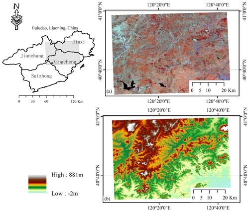
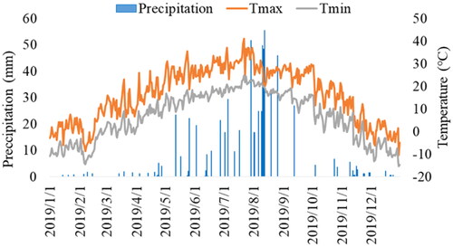
The study area experiences a temperate sub-humid monsoon climate. There is a significant difference in rainfall between the four seasons. We derived the daily precipitation data from Climate Hazards Group Infrared precipitation With Station Data (Version 2.0) which is a 35+ year global precipitation dataset with a resolution of 0.05° (Funk et al. 2015). The daily air temperature (maximum and minimum) is acquired from the Global Land Data Assimilation System (version 2.1) with a resolution of 0.25°. These meteorological data (Figure 2) were used to help explain our results. As we can see, from May to September, there was abundant rainfall and relatively high temperature. We hypothesized that there is no meteorological difference within the study area.

Figure 2. Daily meteorological data for the study area during 2019.

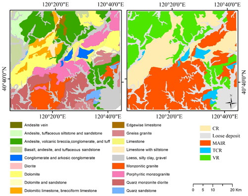
As an important strategic mineral reserve base, Huludao locates in the northeast part of the North China craton and the eastern edge of Yanshan aulacogen. Since Archaean, there have been many strong magmatic activities, so this area has a variety of intrusive rocks and volcanic rocks. We simplified the geologic map and grouped the area into five classes according to the major components (Figure 3): middle acidic intrusive rock (MAIR), carbonate rock (CR), volcanic rock (VR), and terrigenous clastic rock (TCR), the loose deposit was not considered in this study.

Figure 3. The referenced geologic map (modified from the geologic map from the bureau of geology and mineral resources of Liaoning province) and simplified geologic map.

2.2. Data

2.2.1. Sentinel-2

The data used for monitoring vegetation is obtained from S2. The S2 mission consists of two polar-orbiting satellites, phased at 180° to each other. This two-satellite constellation allows a 5-day repeat cycle. S2 data contains 13 spectral bands in visible, red-edge, near-infrared (NIR), and shortwave infrared (SWIR) regions with different resolutions (ESA 2015). European Space Agency provides two different levels (Level-1C and Level-2A) of data for users to download freely. S2 Level-2A products provide the bottom of atmosphere reflectance in UTM/WGS84 projection directly. Hence, the atmosphere correction was already done.

We selected in total 21 images acquired from January to December 2019. Images acquired in June, August, and December were severely contaminated by clouds and not used here. We resampled all bands of S2 to 20 m resolution to balance the computation time and final classification accuracy. All images were clipped to the study area.

2.2.2. Landcover data

The European Space Agency WorldCover 10 m 2020 product was used to provide a non-crop vegetation mask which determined the target area of this study. The WorldCover map generally divides the land cover into 11 classes, including tree, shrub, grass, crop, built-up, bare vegetation, snow/ice, water, wetland, mangroves, and moss/lichen. Due to the local climate factors, crops can be grown in spring and autumn. Different types of crops result in distinct reflectance and growth cycle (Tran et al. 2022). Meanwhile, human interference, such as fertilization and irrigation, can also influence reflectance (Karthikeyan et al. 2020). Thus, we only maintain the tree, shrubs, and grass to study the underlying rocks, and the vegetation mask is demonstrated in (Figure 4(a)).

Figure 4. Vegetation in the study area (a) a mask generated from the WorldCover map; (b) a referenced bedrock map in the vegetated area (c) pictures captured during the field survey in August 2022^nd.

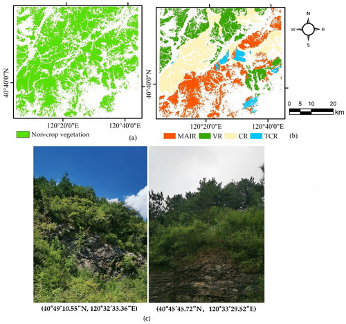
To match the resolution of S2 data, the vegetation mask was resampled into 20 m. The vegetation mask was then used to extract the referenced bedrock map under vegetation (Figure 4(b)). The loose deposit formed in the Quaternary was also not investigated in this study. Vegetation species with different biochemical and biophysical properties result in distinguished spectral performances (Kumar et al. 2001). According to the field survey, the vegetation species are complex with an irregular distribution, and the forest includes both deciduous trees and evergreen trees (Figure 4(c)). Nevertheless, this study does not investigate the effects of vegetation species on vegetation growth, instead, the average performance of vegetation growing on different bedrock was investigated.

3. Methodology

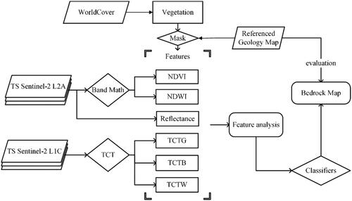
The methodological workflow of this study (Figure 5) mainly consists of 4 parts: (1) extract vegetation spectral features from S2 products; (2) spatiotemporal analysis of vegetation growing on different bedrock; (3) bedrock classification with classifiers; (4) classification accuracy evaluation.

Figure 5. Methodological flowchart of this study.

3.1. Extract and analyze vegetation spectral features

The reflectance of vegetation was derived directly from S2 L2A products. Apart from reflectance, indices including NDVI (Rouse et al. 1974), normalized difference water index (NDWI) (Gao 1996), and components derived from tasseled cap transformation (TCT) were utilized to demonstrate vegetation features.

TCT was first proposed by (Kauth and Thomas 1976) to describe the phenomena of crop growth. TCT generates three typical components, namely Greenness (TCTG), Wetness (TCTW), and Brightness (TCTB). TCT components are found highly correlated with biophysical parameters, and TCTB, TCTG, and TCTW are frequently regarded as a proxy for albedo, vegetation greenness, and soil moisture, respectively (Han et al. 2007; Gómez et al. 2011). As a linear transformation, TCT components are a linear combination of different bands. TCT is scene-independent and can be directly used for multi-scene analysis, thus TCT is widely used in TS applications (Mostafiz and Chang 2018; Macintyre et al. 2020). TCT coefficients are sensor specific. TCT coefficients developed for S2 at-sensor reflectance were listed in Table 1 (Shi and Xu 2019).

Table 1. TCT coefficients for S2 at-sensor reflectance.

	Blue (490nm)	Green (560nm)	Red (665nm)	NIR (842nm)	SWIR (1610nm)	SWIR (2190nm)
TCTB	0.3510	0.3813	0.3437	0.7196	0.2396	0.1949
TCTW	0.2578	0.2305	0.0883	0.1071	−0.7611	−0.5308
TCTG	−0.3599	−0.3533	−0.4734	0.6633	0.0087	−0.2856

The above-mentioned five VIs (NDVI, NDWI, TCTG, TCTB, and TCTW) were calculated via Google Earth Engine. To analyze the temporal variation of vegetation spectral features, we made zonal statistics using the bedrock boundaries derived from the referenced geologic map to extract the temporal statistical mean value of vegetation spectral features for each bedrock. To explore the relationship between the mountain aspect and vegetation VIs, the mountain aspect was calculated using SRTM data. The zonal statistics and calculation of the mountain aspect were carried out via ArcGIS (version 10.5).

We then stacked the reflectance and different combinations of VIs derived from different dates into composite images as input data for classifiers.

3.2. Classification and accuracy assessment

Random forest (RF) developed by (Breiman 2001) is one of the most popular supervised machine-learning classification algorithms that has been widely used in many fields (e.g. agriculture, environment, and geology). We applied RF using the scikit-learn package in Python (Pedregosa et al. 2011). RF classifier contains an ensemble of decision trees with low correlation and the final prediction is determined from all trees according to the majority rule. RF classifier is insensitive to the overfitting problem due to the randomness of samples and variables used for training. We ran the RF classifier with the number of trees equal to 350, and other parameters were set as default. These classifier parameters were fixed throughout the whole experiment.

The importance of different features was calculated by the Gini index algorithm embedded in the RF classifier, and the Gini index of features was measured as the average of the accumulation of the impurity decreases from all trees (Breiman 2001; Menze et al. 2009).

We confirmed the accuracy of the referenced geologic map by field survey, most of the rock outcrops observed are outside the vegetation area, due to the difficulties of collecting samples on mountains with vegetation cover. Therefore, we carefully chose training samples according to the referenced geologic map and the vegetation mask. To avoid the border effect, samples were selected (Figure 6(a)) away from the boundary of the rock, especially the interface between different bedrock. We then randomly generated thousands of test samples according to the referenced geologic map Figure 6(b)). The number of training and test samples was listed in Table 2.

Figure 6. Distribution of training samples (a) and test samples (b), the background image is a red band from the S2 image acquired on July 21^st, 2019. To make the samples clear enough, the boundaries of the sample are made bolder.

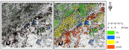
Table 2. The number of samples for training and testing.

	VR	TCR	CR	MAIR	Total
Training (pixel)	4481	1662	4587	4557	15287
Test (pixel)	26219	4379	37340	34779	102717

To evaluate the classification results, normalized confusion matrices, where the element in each cell are percentages calculated by dividing the number of pixels in each cell by the sum of pixels in the entire column, were calculated. Metrics such as overall accuracy (OA), kappa coefficient (kp), producer’s accuracy (PA), and user’s accuracy (UA) were further derived to evaluate the classified results. The classification results were also compared with the reference geologic map visually.

Moreover, the FIM method was also carried out via ENVI software to suppress the vegetation information from the S2 image acquired on July 21^st, 2019. The basic principle and procedures of FIM can refer to (Bachri et al. 2019; Yu et al. 2011; Crippen and Blom 2001). And then the bands after vegetation suppression were directly used as input features for bedrock classification. The classified result using FIM was compared with the results achieved by vegetation features.

4. Results

4.1. Spatiotemporal analysis of VIs

Climate plays an important role in vegetation growth (Pitt and Heady 1978), previous literature demonstrated that climate factors control around 70% variation of NDVI (Ding et al. 2020). Within a limited study area, climate leads to similar change patterns of vegetation growing on different bedrock (Figure 7). Regardless of the type of vegetation, we assumed that the general vegetation growing season was from April 22^nd to October 14^th, according to the acquired dates of S2 images.

Figure 7. NDVI from different dates.

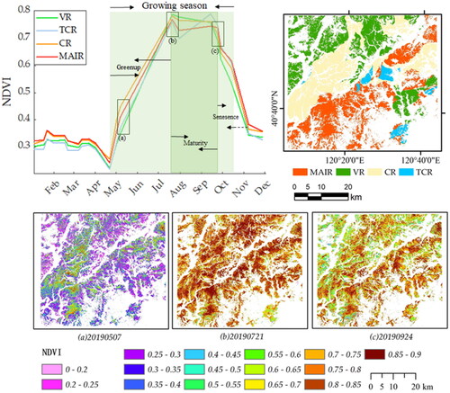
At the start of the growing season, vegetation on CR and MAIR had higher NDVI than that on TCR and VR (Figure 7(a)). On July 21^st, except for TCR, the mean NDVI of all vegetation reached the highest points (corresponding to maturity, with maximum leaf area) and VR had the highest mean NDVI among all rock classes (Figure 7(b)). NDVI of TCR reached the highest point on September 14^th. Since the end of September, the NDVI of vegetation on all bedrock decreased rapidly till November. At the start of senescence, NDVI of VR declined at a faster rate than other rocks (Figure 7(c)). Compared to CR and VR, TCR and MAIR had slightly longer maturity period (the decline of NDVI were later).

NDWI (Figure 8(a)) and TCTG (Figure 8(b)) in the study area are highly correlated with NDVI, and Pearson’s correlation coefficients between them are larger than 0.9 (not shown here). As all these three indices are sensitive to green leaves (the biochemical and biophysical properties), they increased with vegetation greenup and decrease with vegetation senescence. Thus, NDWI and TCTG had very similar change patterns to NDVI that the mean value increased at the end of April and decreased at the end of September. It can be seen that on July 21^st VR had the highest NDWI followed by CR, MAIR, and TCR. We can also note that NDWI of VR, like NDVI of VR, had faster decrement and increment than CR. During the dormant period, TCR had the lowest NDWI. Compared to VR and CR, TCR and GR demonstrated slightly longer periods with high moisture levels.

Figure 8. The temporal change of the mean (a) NDWI; (b) TCTG; (c) TCTW and (d) TCTB on different bedrock.

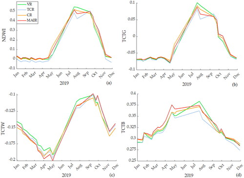
Concerning TCTW (Figure 8(c)), it increased from the end of April to October, then decreased from the middle of October. It can also be seen that TCTW, from January to May, continued to decline. TCTW which is sensitive to moisture information of both soil and vegetation (Crist and Cicone 1984), kept decreasing in the vegetation dormant period, due to the evapotranspiration and little precipitation. Moreover, most vegetation grows in mountainous areas, and topography factors, especially the mountain aspect, have a significant effect on both brightness and moisture. Southeast orientation means more solar radiation and higher temperature, and more evapotranspiration, relative to northwest orientation. Figure 9 demonstrated the influence of the mountain aspect on different VIs, and the mountain aspect can more or less affect all VIs, especially the TCTW which were sensitive to the moisture of both soil and vegetation. In contrast, the influence of the mountain aspect on NDWI, which is sensitive to the moisture of vegetation canopy, is less.

Figure 9. Effect of the mountain aspect on VIs derived from April 22^nd and July 21^st.

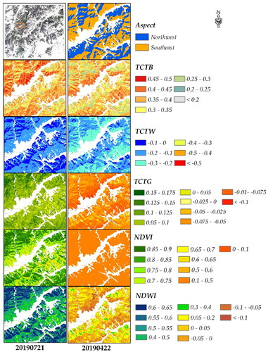
According to the metadata of S2 products, the solar zenith angle varies from around 64° in winter to 42° in spring and autumn, and 27° in summer. The temporal variation of TCTB (Figure 8(d)) can be explained by both vegetation phenology and sun angle. On the one hand, vegetation canopy reflectance has a negative relationship with the solar zenith angle (Ranson et al. 1985), as TCTB can be explained as the sum of surface reflectance (Crist and Cicone 1984), thus TCTB first increase and then decrease within a year as the variation of sun angle. On the other hand, vegetation phenology may also affect the TCTB. Due to the high weight of the NIR band, TCTB is also sensitive to vegetation growth and senescence. Changes in leaf color (from green to red) and dark trunk exposure caused by leaf loss in autumn can lead to a decrease in TCTB, while the growth of green leaves in spring can lead to a TCTB increase (Dymond et al. 2002).

4.2. Bedrock mapping

4.2.1. Using VIs

We compared the performance of different VIs and VI combinations in mapping bedrock. The classification results were compared by OAs and kps (Figure 10(a)). Using all VIs derived from year-round images provided the highest accuracy, with an OA of 69.44% and kp of 0.557, followed by using the combination of NDVI and NDWI (OA = 68.46%, kp = 0.544), and combined use of three TCT components (OA = 67.82%, kp = 0.523). Any single VI used as input data for classifiers showed lower accuracy than the combined use of multi-VIs. Among all VIs, NDVI showed the highest accuracy with an OA of 66.84% and kp of 0.521. TCTW yields the lowest accuracy with an OA of 56.764% and kp of 0.375.

Figure 10. Results of (a) classification using different input features, and selected features refer to VIs derived from the growing season; (b) the importance of VIs derived from different dates.

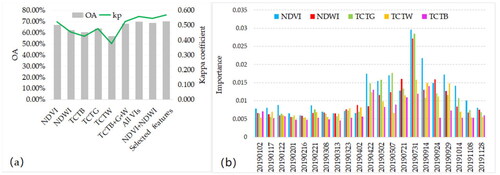
The importance of different VIs derived from different dates (Figure 10(b)). We can see those VIs with importance larger than 0.01 were all from April 22^nd to October 14^th. According to the temporal variation of mean NDVI (Figure 7), it is clear that VIs from the general vegetation growing season were more important for bedrock classification than VIs from vegetation dormant seasons.

Thus, we further only utilized the VIs derived from the growing season to map the bedrock. The result showed a slightly higher OA of 70.06% and kp of 0.567, relative to the classification result using VIs of both growing and dormant seasons. Moreover, on most dates, we can see vegetation greenness (NDVI) played an important role in bedrock classification.

Figure 11 illustrated the classification result achieved by using VIs derived from the growing season. Although the result suffered from ‘pepper’ noise, the classified map showed a roughly right pattern of rocks. The boundaries of rocks are often confused with other rocks. Part of TCR in the middle of the whole area was not well differentiated. VR in the southeast part was mixed with MAIR. The corresponding normalized confusion matrix listed in Table 3, also reveals that TCR was severely mixed with CR and MAIR. TCR had the lowest PA (45.75%) and UA (44.77%), relative to CR, VR, and MAIR.

Figure 11. Classified results from (a) referenced geologic map and (b) selected vegetation features.

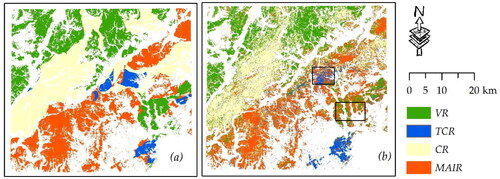
Table 3. Normalized confusion matrix of the classified map calculated from selected vegetation features.

		Ground truth
		VR	TCR	CR	MAIR
Predicted	VR	0.70	0.12	0.12	0.09
	TCR	0.01	0.46	0.02	0.05
	CR	0.17	0.12	0.72	0.14
	MAIR	0.12	0.30	0.15	0.72
	PA	70.25%	45.75%	71.65%	71.77%
	UA	71.50%	44.77%	71.85%	70.80%

4.2.2. Using vegetation reflectance

We then compared the performance of the reflectance of vegetation for classifying bedrock. We had three groups of reflectance, including reflectance in both growing and dormant seasons, reflectance in the growing season, and reflectance in the dormant season. Figure 12(a) demonstrated the OAs and kps of the classified results using these three groups of reflectance. Like the selected vegetation features, reflectance in the growing season showed the best result with an OA of 73.46% and kp of 0.616. While the reflectance in both growing and dormant seasons showed a slightly lower accuracy (OA = 72.62%, kp= 0.603). We can see that reflectance in the dormant season showed the lowest OA of 57.68%, with a kp of 0.358.

Figure 12. Results of (a) classification using reflectance, and selected reflectance refers to reflectance without coastal aerosol and water vapor bands in the growing season); (b) the importance of different bands of S2 for bedrock classification.

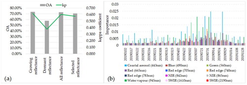
We also measured the importance of the spectral bands of S2 (Figure 12(b)). Similarly, compared to the dormant season, reflectance in the growing season showed a higher importance value. The bands with high importance varied across the growing season. Moreover, Bands in 443 nm and 945 nm, which were sensitive to coastal aerosol and water vapor, respectively, showed higher importance than other bands in most of the dates. To further test the importance of these two bands, we utilized all reflectance from other bands in the vegetation growing season, except for these two bands, to map bedrock. And the classified map had an OA of 70.51% and kp of 0.573, which is comparable to the result from VIs of the growing season (OA of 70.06%).

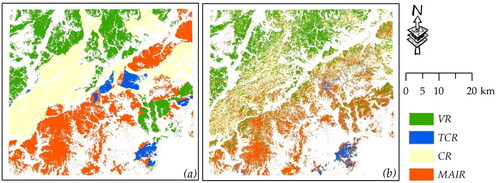
The classification result using reflectance in the growing season was shown in Figure 13. The classified map showed a very similar pattern to the referenced geologic map. Meanwhile, compared to the classified result calculated from VIs of the growing season, it had less noise. According to the normalized confusion matrix (Table 4), TCR still had the lowest PA and UA. However, in general, the UAs and PAs of all rocks showed some improvement, relative to using selected VIs.

Figure 13. Classified results from (a) referenced geologic map and (b) reflectance in the growing season.

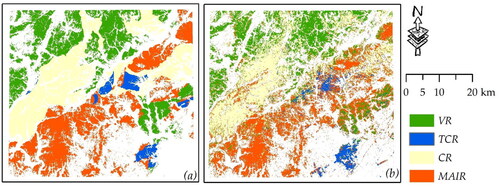
Table 4. Normalized confusion matrix of the classified map calculated from reflectance in the growing season.

		Ground truth
		VR	TCR	CR	MAIR
Predicted	VR	0.75	0.09	0.10	0.08
	TCR	0.01	0.52	0.02	0.04
	CR	0.15	0.14	0.75	0.14
	MAIR	0.09	0.24	0.14	0.74
	PA	74.90%	52.48%	74.56%	74.19%
	UA	75.88%	52.06%	73.51%	74.61%

The classification result using FIM is illustrated in Figure 14, only part of the VR and TCR is tolerably classified, and the classified result of MAIR and CR suffered from severe ‘pepper’ noise. The OA of the classified result was 59.15% and the kp was 0.406. Compared to Figures 11 and 13, it is clear that vegetation spectral features have great potential in mapping bedrock, and the classification accuracy is improved by about 15%, relative to the FIM method.

Figure 14. Classified results from (a) referenced geologic map and (b) bands after vegetation suppression.

5. Discussion

Geologic mapping in vegetated areas using optical remote sensing data is challenging, as the vegetation cover dominates the spectral feature. Thus, additional information such as drainage patterns, elevation, and geobotanical information is usually required to map bedrock underneath vegetation. However, the difference in the phenology of vegetation growing on different bedrock received little attention. This study investigated the potential of using vegetation spectral characteristics (reflectance and different VIs) derived from TS S2 multispectral images to map the underlying bedrock.

The climate, mountain aspect, and sun illumination can all influence vegetation reflectance and VIs, we assume that the effect of these factors on vegetation growing on different bedrock within a limited area is roughly the same (Figures 7 and 8). Some of the subtle differences between the vegetation spectral features can be attributed to the role of bedrock in regulating the climate-vegetation relationship (Cabello et al. 2012; Hubová et al. 2018; Kulkarni et al. 2021; Bai et al. 2021; Nicklas et al. 2021). From May to July, the precipitation was adequate for vegetation growth, the effect of the water-holding capacity of bedrock and the corresponding regolith is not obvious, but after August with decreased precipitation, we notice that compared to CR and VR, TCR and MAIR had slightly longer maturity period (decline of NDVI were later). This can be explained by the stronger water-holding capacity of TCR (mainly sandstone) and MAIR (granite, diorite) than CR (limestone and dolomite) and VR (intermediate-basic volcanic rock) (Eagleson 1982; Jiang et al. 2020; Zhu et al. 2021). Thus, we deduced that the stronger water-holding capacity of TCR and MAIR extends the maturity period of vegetation. Climate and scale constraints may lead to some inconsistent results with previous studies, such as in Karst (or semi-arid) area, plutonic and siliciclastic rocks with strong water-holding capacity have higher NDVI than carbonate rocks (Jiang et al. 2020), while our results demonstrate VR and CR have even higher NDVI than MAIR and TCR. This can occur as a result of the profusion of local rain.

We inferred that the maximum value of NDVI is mainly determined by the number of soluble nutrients that vegetation can extract from soil in the study area. The soluble nutrients (e.g. Ca²⁺, Mg²⁺, Na⁺, K⁺) from parent rock mainly depend on the chemical weathering process, and CR is rated as having high reactivity, followed by VR, MAIR, and TCR (Chuman et al. 2014). Siliceous rocks such as TCR are low in fertility; orthoclase-feldspathic rocks such as MAIR can provide enough K⁺ but little phosphorous (which is important for vegetation growth), Ca²⁺, and Mg²⁺; VR is often rich in nutrients (Webb 1968; Hejda et al. 2022). Compared to iron-rich VR rocks, carbonate rocks have limited phosphorous concentration, especially in arid soil (Porder and Ramachandran 2013), but the associated nutrient-bearing accessory minerals (apatite and biotite) make carbonate rocks have the potential to be fertilizers for plants (Jones et al. 2020). Moreover, carbonate rocks can balance the pH value of soil and resist soil acidification and nutrient degradation processes (Bai et al. 2021).

The vegetation types can cause some confusion among different bedrock, even though we simply take the vegetation’s overall performance into account when mapping bedrock. For instance, the depth of a plant’s roots influences its ability to receive water; deep roots allow access to deeper water, and even if bedrock has a limited capacity to hold water, it can nevertheless support the growth of vegetation (Leone et al. 2020; Liu et al. 2021).

The classification results showed that NDVI and TCTG yield higher accuracy than other indices (Figure 10(a)), this might be because these two indices can describe the difference of vegetation growing above different bedrock with less effect from the slope aspect (Figure 9) and sun angle. The slightly higher OA achieved by NDVI than TCTG can be attributed to the wide separation in the range of NDVI (0.1-0.8) values than TCTG (-0.1-0.1), which provides a more distinct depiction of vegetation at different times. The importance of VIs from different dates further illustrated that indices extracted from the growing season are more useful for bedrock classification than the indices from the dormant period, and the indices extracted from the dormant period can even lead to a mixed result among different rocks (OA decreased by adding indices from the dormant period). This finding emphasizes the importance of vegetation features derived from the growing season for mapping bedrock. Moreover, the higher importance of VIs from July than that from other months may result from the dense vegetation cover, and the direct reflectance from soil and branches decreased the importance of images from the early and late months of vegetation growth (Fathololoumi et al. 2020). The combined use of different indices resulted in higher accuracy than using a single VI, and this may be because these indices composed of different channels describe vegetation from a more holistic perspective. Thus, VI combinations from the growing season are more recommended for bedrock classification, though we did not test all possible VIs.

The OA increased from 70.06% to 73.46% by using reflectance derived from the growing season (Figure 12(a)), instead of using all VIs (Figure 10(a)). From the importance of reflectance and the classified result of using selected bands (Figure 12(b)), it is interesting to see the Coastal aerosol band and Water Vapour band play important roles in mapping bedrock. Both Coastal aerosol and Water Vapour bands are sensitive to the water particles in the air, we deduced that the high importance of these two bands is highly related to the humid environment of the study area (located in a coastal city). And by adding these two bands, the reflectance achieved higher OA (increased by around 3%). But the usefulness of these two bands in mapping bedrock under vegetation still needs to be further investigated, experiments carried out inland away from the sea should be considered in the future.

In contrast, the classified result from FIM has the lowest OA (59.15%) and there is severe confusion and noise in the classified bedrock map. This may be because the impacts of vegetation cannot be totally eliminated in highly vegetated areas by FIM (Bachri et al. 2019; Liu et al. 2018). Although studies using vegetation spectral features to classify bedrock underneath vegetation are rare and hard to establish discussion, attempts have been made to map soil properties using vegetation spectral features (Mahmoudabadi et al. 2017; Demattê et al. 2017).

Classified maps from both VIs and reflectance are suffered from confusion between different rocks, this can be caused by several factors. The difference caused by the mountain aspect within one bedrock class will aggravate the confusion between different bedrock, especially between rocks with subtle differences. Vegetation types, diversity, and spatial distribution heterogeneity can also lead to confusion in the final classified maps. Meanwhile, we grouped bedrock into different classes, but the composition of the regolith can more or less be similar and result in similar vegetation growth patterns.

Overall, the use of TS vegetation features derived from the growing season using S2 images can give a reasonable bedrock map, but the potential of vegetation features in distinguishing other types of bedrock still needs further exploration. Our results show that S2 data has great potential in mapping bedrock in dense vegetation areas at regional scales, and the free acquisition and extensive coverage of the S2 data make it possible to be applied at national and global scales. The potential still needs further exploration. Optical remote sensing images can be disturbed by cloud and cloud shadows, especially in the vegetation growing season with abundant precipitation. Therefore, we lose some detailed information. The harmonization between S2 and Landsat-8 data improves the frequency of observation, which may further improve the accuracy. Moreover, the long observation of S2 data also provides the possibility of replacing the cloud-contaminated data with data from other years. In addition, the classified bedrock map can serve as a baseline for evaluating the accuracy of the referenced map. Traditionally, regional geologic maps usually are drawn by intensive field investigation, but the inaccessible places still limit the map accuracy. The inconsistency between our result and the referenced map highlights the places that need to be investigated. Meanwhile, the classified map offers more materials for forest or grass managers to make decisions, due to the close relationship between vegetation productivity and bedrock (Maimouni et al. 2021).

6. Conclusion

This study investigates the performance of using vegetation spectral features (VIs and reflectance) derived from TS S2 images directly to classify the bedrock (VR, CR, TCR, and MAIR) underneath dense vegetation. The classified results were assessed by confusion matrices and the corresponding metrics.

Among all the VIs, NDVI showed the best classification result with an OA of 66.84% and kp of 0.521. The combined use of all VIs resulted in a higher OA of 69.44% and kp of 0.557. An optimized classification result can be achieved by using all VIs derived only from the growing season, with an OA of 70.06% and kp of 0.567. As for vegetation spectral reflectance, the highest OA was achieved by using reflectance only from the growing season with OA of 73.46% and kp of 0.616. Compared with the FIM method (OA = 59.15%, and kp 0.406), the classification accuracy is improved by about 15%, using TS vegetation spectral features.

In summary, our results demonstrate the close relationship between vegetation growth and lithological characteristics can be captured by TS S2 images, and the vegetation spectral features derived from S2 products have great potential in bedrock classification. This paper proposes a new way to map bedrock with dense vegetation cover.

Acknowledgement

The authors would also like to thank the anonymous reviewers for their valuable comments to improve the manuscript.

Disclosure statement

No potential conflict of interest was reported by the author(s).

Additional information

Funding

This study was funded by the National Natural Science Foundation of China (Project No. 42130805).

References

- Adiri Z, Lhissou R, El Harti A, Jellouli A, Chakouri M. 2020. Recent advances in the use of public domain satellite imagery for mineral exploration: a review of Landsat-8 and Sentinel-2 applications. Ore Geol Rev. 117:103332. doi: 10.1016/j.oregeorev.2020.103332.
- Bachri I, Hakdaoui M, Raji M, Teodoro AC, Benbouziane A. 2019. Machine learning algorithms for automatic lithological mapping using remote sensing data: a case study from Souk Arbaa Sahel, Sidi Ifni Inlier, Western Anti-Atlas, Morocco. IJGI. 8(6):248. doi: 10.3390/ijgi8060248.
- Bai Y, He Q, Liu Z, Wu Z, Xie S. 2021. Soil nutrient variation impacted by ecological restoration in the different lithological Karst Area, Shibing, China. Glob Ecol Conserv. 25:e01399. doi: 10.1016/j.gecco.2020.e01399.
- Black M, Riley TR, Ferrier G, Fleming AH, Fretwell PT. 2016. Automated lithological mapping using airborne hyperspectral thermal infrared data: a case study from Anchorage Island, Antarctica. Remote Sens Environ. 176:225–241. doi: 10.1016/j.rse.2016.01.022.
- Bradbury DE. 1944. Vegetation as an indicator of rock types in the Northern Swisshelm Mountains, Southeastern Arizona. Arizona: The University of Arizona.
- Breiman LEO. 2001. Random forests. Mach Learn. 45(1):5–32. doi: 10.1023/A:1010933404324.
- Broge NH, Leblanc E. 2001. Comparing prediction power and stability of broadband and hyperspectral vegetation indices for estimation of green leaf area index and canopy chlorophyll density. Remote Sens Environ. 76(2):156–172. doi: 10.1016/S0034-4257(00)00197-8.
- Cabello J, Alcaraz-Segura D, Ferrero R, Castro AJ, Liras E. 2012. The role of vegetation and lithology in the spatial and inter-annual response of EVI to climate in drylands of Southeastern Spain. J Arid Environ. 79(April):76–83. doi: 10.1016/j.jaridenv.2011.12.006.
- Chuman T, Gürtlerová P, Hruška J, Adamová M. 2014. Geochemical reactivity of rocks of the Czech Republic. J Maps. 10(2):341–349. doi: 10.1080/17445647.2013.867418.
- Crippen RE, Blom RG. 2001. Unveiling the lithology of vegetated terrains in remotely sensed imagery. Photogramm Eng Remote Sens. 67(8):935–943.
- Crist EP, Cicone RC. 1984. A physically-based transformation of thematic mapper data-the TM Tasseled Cap. IEEE Trans Geosci Remote Sens. GE-22(3):256–263. doi: 10.1109/TGRS.1984.350619.
- Demattê JA, Sayão VM, Rizzo R, Fongaro CT. 2017. Soil class and attribute dynamics and their relationship with natural vegetation based on satellite remote sensing. Geoderma. 302(May):39–51. doi: 10.1016/j.geoderma.2017.04.019.
- Ding Y, Li Z, Peng S. 2020. Global analysis of time-lag and -accumulation effects of climate on vegetation growth. Int J Appl Earth Observ Geoinf. 92(June):102179. doi: 10.1016/j.jag.2020.102179.
- Dymond CC, Mladenoff DJ, Radeloff VC. 2002. Phenological differences in tasseled cap indices improve deciduous forest classification. Remote Sens Environ. 80(3):460–472. doi: 10.1016/S0034-4257(01)00324-8.
- Eagleson PS. 1982. Ecological optimality in water-limited natural soil-vegetation systems 1. Theory and hypothesis. Water Resour Res. 18(2):325–340. doi: 10.1029/WR018i002p00325.
- Erinjery JJ, Singh M, Kent R. 2018. Mapping and assessment of vegetation types in the tropical rainforests of the Western Ghats using multispectral Sentinel-2 and SAR Sentinel-1 satellite imagery. Remote Sens Environ. 216(October):345–354. doi: 10.1016/j.rse.2018.07.006.
- ESA. 2015. SENTINEL-2 User Handbook. doi: 10.13128/REA-22658.
- Fathololoumi S, Vaezi AR, Kazem Alavipanah S, Ghorbani A, Saurette D, Biswas A. 2020. Improved digital soil mapping with multitemporal remotely sensed satellite data fusion: a case study in Iran. Sci Total Environ. 721:137703. doi: 10.1016/j.scitotenv.2020.137703.
- Feng J, Rivard B, Rogge D, Sánchez-Azofeifa A. 2013. The longwave infrared (3-14μm) spectral properties of rock encrusting lichens based on laboratory spectra and airborne SEBASS imagery. Remote Sens Environ. 131:173–181. doi: 10.1016/j.rse.2012.12.018.
- Frampton WJ, Dash J, Watmough G, Milton EJ. 2013. Evaluating the capabilities of Sentinel-2 for quantitative estimation of biophysical variables in vegetation. ISPRS J Photogramm Remote Sens. 82(August):83–92. doi: 10.1016/j.isprsjprs.2013.04.007.
- Fraser SJ, Green AA. 1987. A software defoliant for geological analysis of band ratios. Int J Remote Sens. 8(3):525–532. doi: 10.1080/01431168708948659.
- Funk C, Peterson P, Landsfeld M, Pedreros D, Verdin J, Shukla S, Husak G, Rowland J, Harrison L, Hoell A, et al. 2015. The climate hazards infrared precipitation with stations - a new environmental record for monitoring extremes. Sci Data. 2:150066. doi: 10.1038/sdata.2015.66.
- Gao B-C. 1996. NDWI—a normalized difference water index for remote sensing of vegetation liquid water from space. Remote Sens Environ. 58(3):257–266. doi: 10.1016/S0034-4257(96)00067-3.
- Ghosh T, Hazra S, Kumar Das A. 2022. Potential of ALOS-2 PALSAR-2 stripmap data for lithofacies identification and geological lineament mapping in vegetated fold-thrust belt of Nagaland, India. Adv Space Res. 69(4):1840–1862. doi: 10.1016/j.asr.2021.09.007.
- Gómez C, White JC, Wulder MA. 2011. Characterizing the state and processes of change in a dynamic forest environment using hierarchical spatio-temporal segmentation. Remote Sens Environ. 115(7):1665–1679. doi: 10.1016/j.rse.2011.02.025.
- Grebby S, Cunningham D, Naden J, Tansey K. 2010. Lithological mapping of the Troodos ophiolite, Cyprus, using airborne LiDAR topographic data. Remote Sens Environ. 114(4):713–724. Elsevier doi: 10.1016/j.rse.2009.11.006.
- Grebby S, Cunningham D, Tansey K, Naden J. 2014. The impact of vegetation on lithological mapping using airborne multispectral data: a case study for the north Troodos Region, Cyprus. Remote Sens. 6(11):10860–10887. doi: 10.3390/rs61110860.
- Grebby S, Field E, Tansey K, Yu B, Galvao LS, Thenkabail PS. 2016. Evaluating the use of an object-based approach to lithological mapping in vegetated terrain. Remote Sens. 8(10):843. doi: 10.3390/RS8100843.
- Grebby S, Naden J, Cunningham D, Tansey K. 2011. Integrating airborne multispectral imagery and airborne LiDAR data for enhanced lithological mapping in vegetated terrain. Remote Sens Environ. 115(1):214–226. Elsevier doi: 10.1016/j.rse.2010.08.019.
- Han T, Wulder MA, White JC, Coops NC, Alvarez MF, Butson C. 2007. An efficient protocol to process Landsat images for change detection with tasselled cap transformation. IEEE Geosci Remote Sens Lett. 4(1):147–151. doi: 10.1109/LGRS.2006.887066.
- Harris JR, Rogge D, Hitchcock R, Ijewliw O, Wright D. 2005. Mapping lithology in Canada ‘ s Arctic: Application of hyperspectral data using the minimum noise fraction transformation and matched filtering. Can J Earth Sci. 42(12):2173–2193. doi: 10.1139/e05-064.
- Hejda M, Čuda J, Pyšková K, Zambatis G, Foxcroft LC, MacFadyen S, Storch D, Tropek R, Pyšek P. 2022. Water availability, bedrock, disturbance by herbivores, and climate determine plant diversity in South-African Savanna. Sci Rep. 12(1):338. doi: 10.1038/s41598-021-02870-3.
- Hubová P, Tejnecký V, Češková M, Borůvka L, Němeček K, Drábek O. 2018. Behaviour of aluminium in forest soils with different lithology and herb vegetation cover. J Inorg Biochem. 181:139–144. doi: 10.1016/j.jinorgbio.2017.09.017.
- Jiang Z, Liu H, Wang H, Peng J, Meersmans J, Green SM, Quine TA, Wu X, Song Z. 2020. Bedrock geochemistry influences vegetation growth by regulating the regolith water holding capacity. Nat Commun. 11(1):2392. doi: 10.1038/s41467-020-16156-1.
- Jones JM, Guinel FC, Antunes PM. 2020. Carbonatites as rock fertilizers: a review. Rhizosphere. 13:100188. doi: 10.1016/j.rhisph.2020.100188.
- Joswig JS, Wirth C, Schuman MC, Kattge J, Reu B, Wright IJ, Sippel SD, Rüger N, Richter R, Schaepman ME, et al. 2022. Climatic and soil factors explain the two-dimensional spectrum of global plant trait variation. Nat Ecol Evol. 6(1):36–50. doi: 10.1038/s41559-021-01616-8.
- Karthikeyan L, Chawla I, Mishra AK. 2020. A review of remote sensing applications in agriculture for food security: crop growth and yield, irrigation, and crop losses. J Hydrol. 586:124905. doi: 10.1016/j.jhydrol.2020.124905.
- Kauth RJ, Thomas GS. 1976. The tasselled cap – A graphic description of the spectral-temporal development of agricultural crops as seen by landsat. In LARS Symposia, p. 159. Purdue University, West Lafayette, Indiana: IEEE.
- Kulkarni A, Shetti R, Shigwan BK, Vijayan S, Datar MN. 2021. What determines vegetation on rock outcrops of the Western Ghats: the macro-environment or lithotype? Folia Geobot. 56(2–3):149–165. doi: 10.1007/s12224-021-09399-3.
- Kumar L, Schmidt K, Dury S, Skidmore A. 2001. Imaging Spectrometry: basic Principles and Prospective Applications. p. 111–155. Dordrecht: Springer.
- Kycko M, Zagajewski B, Kluczek M, Tardà A, Pineda L, Palà V, Corbera J. 2022. Sentinel-2 and AISA airborne hyperspectral images for mediterranean shrubland mapping in Catalonia. Remote Sens. 14(21):5531. doi: 10.3390/rs14215531.
- Langford RL. 2015. Temporal merging of remote sensing data to enhance spectral regolith, lithological and alteration patterns for regional mineral exploration. Ore Geol Rev. 68:14–29. doi: 10.1016/j.oregeorev.2015.01.005.
- Leone JD, Holbrook WS, Riebe CS, Chorover J, Ferré TP, Carr BJ, Callahan RP. 2020. Strong slope-aspect control of regolith thickness by bedrock foliation. Earth Surf Process Landforms. 45(12):2998–3010. doi: 10.1002/esp.4947.
- Liu H, Dai J, Xu C, Peng J, Wu X, Wang H. 2021. Bedrock-associated belowground and aboveground interactions and their implications for vegetation restoration in the Karst critical zone of Subtropical Southwest China. Prog Phys Geogr. 45(1):7–19. doi: 10.1177/0309133320949865.
- Liu L, Ji M, Buchroithner M. 2018. A case study of the forced invariance approach for soil salinity estimation in vegetation-covered terrain using airborne hyperspectral imagery. IJGI. 7(2):48. doi: 10.3390/ijgi7020048.
- Macintyre P, van Niekerk A, Mucina L. 2020. Efficacy of multi-season Sentinel-2 imagery for compositional vegetation classification. Int J Appl Earth Observ Geoinf. 85:101980. doi: 10.1016/j.jag.2019.101980.
- Mahanta P, Maiti S. 2018. Regional scale demarcation of alteration zone using ASTER imageries in South Purulia Shear Zone, East India: Implication for mineral exploration in vegetated regions. Ore Geol Rev. 102(August):846–861. doi: 10.1016/j.oregeorev.2018.07.028.
- Mahmood TH, Hasan K, Akhter SH. 2019. Lithologic mapping of a forested montane Terrain from Landsat 5 TM image. Geocarto Int. 34(7):750–768. doi: 10.1080/10106049.2018.1434688.
- Mahmoudabadi E, Karimi A, Haghnia GH, Sepehr A. 2017. Digital soil mapping using remote sensing indices, terrain attributes, and vegetation features in the Rangelands of Northeastern Iran. Environ Monit Assess. 189(10):500. doi: 10.1007/s10661-017-6197-7.
- Maimouni S, Daghor L, Oukassou M, Moutaki SE, Lhissou R. 2021. Evaluate the effect of topographic factors and lithology on forest cover distribution: a case study of the Moroccan high atlas. Environ Model Assess. 26(5):787–801. doi: 10.1007/s10666-021-09785-3.
- Manap HS, San BT. 2022. Data integration for lithological mapping using machine learning algorithms. Earth Sci Inform. 15(3):1841–1859. doi: 10.1007/s12145-022-00826-3.
- Martin MH, Coughtrey PJ. 1982. Biological monitoring of heavy metal pollution. Dordrecht: Springer.
- McCormick EL, Dralle DN, Hahm WJ, Tune AK, Schmidt LM, Chadwick KD, Rempe DM. 2021. Widespread woody plant use of water stored in bedrock. Nature. 597(7875):225–229. S doi: 10.1038/s41586-021-03761-3.
- Meer FVD, De Jong SM. 2000. Improving the results of spectral unmixing of landsat thematic mapper imagery by enhancing the orthogonality of end-members. Int J Remote Sens. 21(15):2781–2797. doi: 10.1080/01431160050121249.
- Menze BH, Kelm BM, Masuch R, Himmelreich U, Bachert P, Petrich W, Hamprecht FA. 2009. A comparison of random forest and its Gini importance with standard chemometric methods for the feature selection and classification of spectral data. BMC Bioinf. 10:213. doi: 10.1186/1471-2105-10-213.
- Mostafiz C, Chang NB. 2018. Tasseled cap transformation for assessing hurricane landfall impact on a coastal watershed. Int J Appl Earth Observ Geoinf. 73:736–745. doi: 10.1016/j.jag.2018.08.015.
- Mwaniki MW, Matthias MS, Schellmann G. 2015. Application of remote sensing technologies to map the structural geology of Central Region of Kenya. IEEE J Sel Top Appl Earth Observ Remote Sens. 8(4):1855–1867. doi: 10.1109/JSTARS.2015.2395094.
- Nicklas L, Walde J, Wipf S, Lamprecht A, Mallaun M, Rixen C, Steinbauer K, Theurillat J-P, Unterluggauer P, Vittoz P, et al. 2021. Climate change affects vegetation differently on siliceous and calcareous summits of the European alps. Front Ecol Evol. 9(April):1–15. doi: 10.3389/fevo.2021.642309.
- Ott RF. 2020. How lithology impacts global topography, vegetation, and animal biodiversity: a global-scale analysis of mountainous regions. Geophys Res Lett. 47(20):e2020GL088649. doi: 10.1029/2020GL088649.
- Paradella WR, Bignelli PA, Veneziani P, Pietsch RW, Toutin T. 1997. Airborne and spaceborne synthetic aperture radar (SAR) integration with Landsat TM and gamma ray spectrometry for geological mapping in a tropical rainforest environment, the Mineral Province, Brazil. Int J Remote Sens. 18(7):1483–1501. doi: 10.1080/014311697218232.
- Pedregosa F, Varoquaux G, Gramfort A, Michel V, Thirion B, Grisel O. 2011. Scikit-Learn: machine learning in Python. J Mach Learn Res. 12:2825–2830. doi: 10.1289/EHP4713.
- Pitt MD, Heady HF. 1978. Responses of annual vegetation to temperature and rainfall patterns in Northern California. Ecology. 59(2):336–350. doi: 10.2307/1936378.
- Porder S, Ramachandran S. 2013. The phosphorus concentration of common rocks-a potential driver of ecosystem P status. Plant Soil. 367(1-2):41–55. doi: 10.1007/s11104-012-1490-2.
- Qiao Y, Chen H, Jiang Y. 2020. Quantifying the impacts of lithology on vegetation restoration using a random forest model in a Karst Trough Valley, China. Ecol Eng. 156:105973. doi: 10.1016/j.ecoleng.2020.105973.
- Ranson KJ, C ST, Daughtry LL, Biehl, ME, Bauer. 1985. Sun-view angle effects on reflectance factors of corn canopies. Remote Sens Environ. 18(2):147–161. doi: 10.1016/0034-4257(85)90045-8.
- Robertson KM, Milliken RE, Li S. 2016. Estimating mineral abundances of clay and gypsum mixtures using radiative transfer models applied to visible-near infrared reflectance spectra. Icarus. 277(October):171–186. doi: 10.1016/j.icarus.2016.04.034.
- Rodriguez-Gomez C, Kereszturi G, Reeves R, Rae A, Pullanagari R, Jeyakumar P, Procter J. 2021. Lithological mapping of Waiotapu geothermal field (New Zealand) using hyperspectral and thermal remote sensing and ground exploration techniques. Geothermics. 96(July):102195. doi: 10.1016/j.geothermics.2021.102195.
- Rouse JW, Jr., Haas RH, Schell JA, Deering DW. 1974. Monitoring vegetation systems in the great plains with ERTS. Goddard Space Flight Center 3d ERTS-1 Symptoms, p. 309–317. Washington, D.C.: NASA. https://ntrs.nasa.gov/search.jsp?R=19740022614.
- Shi T, Xu H. 2019. Derivation of tasseled cap transformation coefficients for Sentinel-2 MSI at-sensor reflectance data. IEEE J Sel Top Appl Earth Observ Remote Sens. 12(10):4038–4048. doi: 10.1109/JSTARS.2019.2938388.
- Shirmard H, Farahbakhsh E, Müller RD, Chandra R. 2022. A review of machine learning in processing remote sensing data for mineral exploration. Remote Sens Environ. 268:112750. doi: 10.1016/j.rse.2021.112750.
- Siegal BS, Goetz AFH. 1977. Effect of vegetation on rock and soil type discrimination. Photogramm Eng Remote Sens. 43(2):191–196.
- Taylor P. 2014. Geobotanical and soil spectral investigation for rock discrimination in the ‘Caatinga’ environment (Brazil) based on multitemporal remote sensing data. Can J Remote Sens. 21(1):37–41. doi: 10.1080/07038992.1995.10874596.
- Tran KH, Zhang HK, Mcmaine JT, Zhang X, Luo D. 2022. 10 m Crop type mapping using Sentinel-2 reflectance and 30 m cropland data layer product. Int J Appl Earth Observ Geoinf. 107:102692. doi: 10.1016/j.jag.2022.102692.
- Tsui CC, Chen ZS, Hsieh CF. 2004. Relationships between soil properties and slope position in a lowland rain forest of Southern Taiwan. Geoderma. 123(1–2):131–142. doi: 10.1016/j.geoderma.2004.01.031.
- Wang R, Lin J, Zhao B, Li L, Xiao Z, Pilz J. 2018. Integrated approach for lithological classification using ASTER imagery in a shallowly covered region-the Eastern Yanshan Mountain of China. IEEE J Sel Top Appl Earth Observ Remote Sens. 11(12):4791–4807. doi: 10.1109/JSTARS.2018.2879493.
- Warner T, Levandowski D, Bell R, Cetin H. 1994. Rule-based geobotanical classification of topographic, aeromagnetic, and remotely sensed vegetation community data. Remote Sens Environ. 50(1):41–51. doi: 10.1016/0034-4257(94)90093-0.
- Webb LJ. 1968. Environmental relationships of the structural types of Australian Rain forest vegetation. Ecol Soc Am Stable. 49(2):296–311. doi: 10.2307/1934459.
- Wilson MJ. 2019. The importance of parent material in soil classification: a review in a historical context. Catena. 182(May):104131. doi: 10.1016/j.catena.2019.104131.
- Yu L, Porwal A, Holden EJ, Dentith MC. 2011. Suppression of vegetation in multispectral remote sensing images. Int J Remote Sens. 32(22):7343–7357. doi: 10.1080/01431161.2010.523726.
- Zhong F, Xu X, Li Z, Zeng X, Yi R, Luo W, Zhang Y, Xu C. 2022. Relationships between lithology, topography, soil, and vegetation, and their implications for Karst vegetation restoration. Catena. 209(P1):105831. doi: 10.1016/j.catena.2021.105831.
- Zhu X, Liu H, Wu L, Liang B, Liu F, He W. 2021. Impact of bedrock geochemistry on vegetation productivity depends on climate dryness in the Guizhou Karst of China. Prog Phys Geogr. 45(1):20–32. doi: 10.1177/0309133320936085.
- Zou X, Mõttus M. 2017. Sensitivity of common vegetation indices to the Canopy structure of field crops. Remote Sens. 9(10):994. doi: 10.3390/rs9100994.