Applicability study of four atmospheric correction methods in the remote sensing of lake water color

Abstract

Due to the complexity of spectral characteristics for inland lake water, high-precision atmospheric correction methods play an essential role in remote sensing. This research conducted atmospheric correction on the Tiande lake zone in Zhengzhou, China based on Zhuhai-1, Sentinel-2, Planet, and GF-2 images using four methods (QUAC, Dark Subtract, Fast Line-of-sight Atmospheric Analysis of Spectral Hypercubes (FLAASH) and 6S). In doing so, water reflectance can be extracted and compared with the data measured from a ground-based spectrometer. The analysis indicates that the FLAASH method has best applicability to Zhuhai-1 and Sentinel-2 images; while 6S method shows best applicability to Planet and GF-2 images. The comparison of single-band images indicates that the four atmospheric correction approaches used in different images are proven to be applicable to construction of sensitive wavebands of a water body inversion model in the Tiande lake zone. The correction results of four types of images prove that FLAASH and 6S are more applicable to lake water color remote sensing inversion.

Keywords:

• Zhuhai-1
• sentinel-2
• planet
• GF-2
• atmospheric correction
• lake

1. Introduction

At present, remote sensing of lake water color has been developed from ground-based remote sensing and medium-resolution satellite to the use of high-resolution spectral unmanned aerial vehicle (UAV) technology. Algorithmic power has been developed into machine learning algorithms for cloud computing (Wang and Dou 1998; Duan et al. 2022). Atmospheric correction is a key stage in the processing of remote sensing images. By eliminating influences of factors including the atmosphere and light on ground reflections, the true water reflectance of lake water body can be determined. There are multiple atmospheric correction (AC) methods available at present. How to find an atmospheric correction method more suitable for processing water color remote sensing images is an issue worthy of discussion (Hu et al. 2014; Liu et al. 2016; Doxani et al. 2023); Radiation transmission models are currently the most commonly used atmospheric correction methods, including 6S (second simulation of satellite signal in the solar spectrum), MODTARN (moderate resolution transmission), FLAASH (Fast Line-of-Fight). Atmospheric Analysis of Spectral Hypercubes, ACORN (atmospheric correction now), etc (Zheng and Zeng 2004; Li et al. 2018). Wang et al. (2019) investigated the performance of AC methods on processing of remote sensing image data for Lake Hongze, Lake Taihu, and Lake Chaohu based on Landsat-8 images. The results indicated that Second Simulation of a Satellite Signal in the Solar Spectrum-Vector (6SV) algorithm among the terrestrial AC algorithms offered the best ratio of remote sensing reflectance and wave bands. Pan et al. (2022) estimated ten types of atmospheric correction methods based on Sentinel-2 and Landsat-7 images and qualitatively analyzed the influence of proximity effect on the AC methods. Based on Sentinel-2 images, Mu et al. (2021) utilized three atmospheric methods (Atmospheric Correction for OLI lite model (ACOLITE), FLAASH and the Case 2 Regional Coast Color processor (C2RCC)) to perform AC studies of inland lakes. Martins et al. (2017) evaluated AC methods based on Sentinel-2A images of Amazon floodplain lakes. Li et al. (2021) used five types of AC methods (Sentinel 2 correction (Sen2cor), 6S, FLAASH, QUAC, and ACOLITE) based on Sentinel-2 images to undertake AC research into Lake Poyang. The results indicate that the AC performance of Sen2cor and FLAASH methods is superior to other methods. Tian et al. (2021) employed three models (FLAASH, QUAC, and the Atmospheric and Topographic Correction model (ATCOR)) to perform AC of WorldView-3 satellite images. They undertook a comparative analysis of visual effects, evaluation indices, ground object spectral curves, and classification accuracy of images before and after corrections had been applied. The results reveal that FLAASH and ATCOR both show good AC correction effect compared with the QUAC model. At present, the atmospheric correction research on satellite images at home and abroad mainly focuses on Sentinel-2, Landsat 7, Landsat 8, GF-1 and other images, while there are relatively few atmospheric correction studies on Zhuhai No. 1 image, Planet image and GF-2 image. And most existing studies about AC algorithms mainly focus on large-scale lakes. Some AC algorithms applicable to oceanic areas are difficult to apply in inland lakes, thus making it necessary to explore the applicability of general AC methods to lake regions.

Based on Zhuhai-1 hyperspectral images, Sentinel-2 images, Planet images, and GF-2 images, this research respectively adopts QUAC, Dark Subtract, FLAASH, and 6S models to perform AC processing of images of the Tiande Lake zone in Zhengzhou, China. The data obtained are compared with measured spectral data to estimate the performance of these four AC models. In doing so, the applicability of these models to lake water color remote sensing can be identified.

2. Research zone and data

2.1. Research zone and measure spectral data

Tiande Lake is situated at the Zhengzhou High Tech Zone, which is the core zone of Binhe Park of the Xushui River. This terrain of this zone is flat, encompassing a branch of the Jialu.

River that flows through the confluence of Huiji District (Guxing Town Section) and Suo River. The lake covers an area of about 0.306 km², and is classified as a Class V water body with a water level of between 2 and 5 m (Figure 1).

Figure 1. Geographical location and sampling point distribution in the study area (Planet).

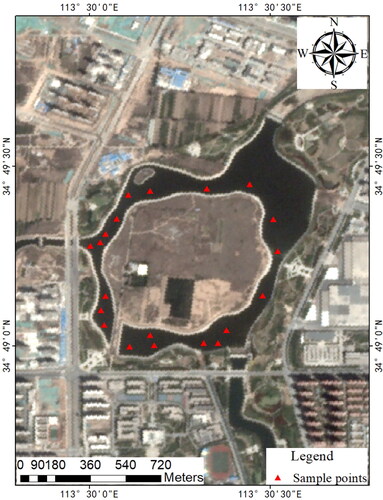
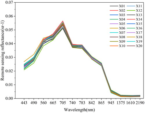
There are 20 measured sampling spectral points of lake surface, which are circumferentially distributed around the lake (Figure 1). The measured data collection used in this article is dated 18 April 2019, the spectral measurement was fulfilled using a PSR3500 handheld spectrometer with a wavelength of 325–2500 nm. The hyperspectral data acquisition process is repeated three times at each sampling point and the remote sensing reflectance of lake water can be obtained using post-processing software. The average value of three remote sensing data for each sampling point is taken as the final reflectance value of the current spectral measurement point, which is used as the data for verifying AC results of different models (Figure 2).

Figure 2. Measured spectral data.

2.2. Remote sensing data

The Zhuhai-1 hyperspectral satellite is a hyperspectral satellite launched by Zhuhai Orbital Aerospace Science and Technology Co., Ltd, having 32 effective imaging bands, spatial resolution of 10 m, and spectral resolution of 2.5 nm. This experiment utilized hyperspectral images recorded on 1 June 2019. It can be found that there are a small portion of clouds in the atmosphere of the research region and its surrounding area.

Sentinel-2 is a high-resolution multispectral imaging satellite developed by the European Space Agency. It consists of two satellites 2 A and 2B and 13 spectral wavebands. In addition, its spectral ranges cover RGB, near infra-red (NIR), and shortwave infrared (SWIR) with ground resolutions of 10, 20, and 60 m respectively. The revisit period and spatial resolution of Sentinel-2 offer more opportunities for exploring water eutrophication monitoring, land-cover changes, and crop growth (Guan et al. 2022; Luo et al. 2022; Xie et al. 2022). This experiment selected S2A images recorded on 18 April 2019, covering the zone ranging between 113° 11′ to 114° 21′ E, 34° 12′ to 35° 13′ N. The cloud coverage in the images is 0.0509%.

The Planet satellite demonstrates characteristics such high resolution, high frequency, and full coverage capability. It is the largest micro-satellite group in the world, consisting of hundreds of Dove satellites, encompassing visible light and NIR wavebands with a spatial resolution of 3–4 m. In this experiment, Planet 1B images recorded on 17 April 2019 are selected. The sky in the area of interest and its surrounds is free from cloud.

GF-2 is a civil optical remote sensing satellite independently developed in China: it contains 4-m multispectral, and 1-m panchromatic high-resolution imaging capability. This experiment selected an image recorded on 16 April 2019 (at a time of slight cloud coverage).

3. Research method

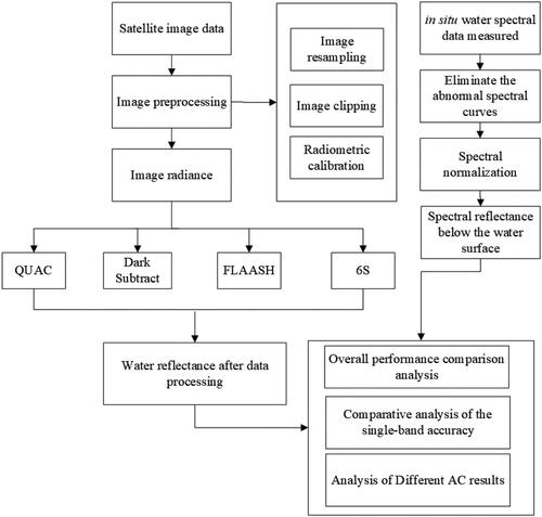
This research adopts four methods which are QUAC, Dark Subtract, FLAASH, and 6S to perform AC experiments on Zhuhai-1 hyperspectral images, Sentinel-2 images, Planet images, and GF-2 images. The data obtained are compared with measured spectral data to estimate AC accuracies of these methods. The specific technical roadmap is illustrated in Figure 3.

Figure 3. Technical roadmap.

In order to evaluate the atmospheric correction effect, the coefficient of determination R², root mean square error (RMSE), and mean relative error (MRE) are used to test the differences between the atmospheric correction results and the measured data. (1) $$R^2=\frac{\sum _{\mathrm{i}=1}^n{({y^{\prime }}_i-\overline{y})}^2}{\sum _{\mathrm{i}=1}^n{(y_i-\overline{y})}^2}$$(1) (2) $$\mathit{RMSE}=\sqrt{\frac{\sum _{\mathrm{i}=1}^n{(y_i-{y^{\prime }}_i)}^2}{n-1}}$$(2) (3) $$\mathit{MRE}=\frac{\sum _{i=1}^n\frac{\left|{y^{\prime }}_i-y_i\right|}{y_i}\times 100\%}{n}$$(3)

In the above formula, ${y^{\prime }}_i$ indicates the reflectivity of the $i_{th}$ band after atmospheric correction; $y_i$ indicates measured reflectivity in the $i_{th}$ band; $n$ represents the number of sample points; $\overline{y}$ represents the average of the measured reflectivity.

3.1. QUAC AC method

The QUAC method automatically acquires relative spectral information from surface objects in images based on dark target models, further obtaining empirical values to fulfil AC. At present, the QUAC model supports atmospheric correction of multispectral and hyperspectral images in the visible light, near-infrared, and shortwave infrared spectral ranges, and only needs to provide the center wavelength information and radiometric calibration of each band of the multispectral and hyperspectral sensor using the on-site method (Bernstein et al. 2012; Guo and Zeng 2012). Compared with other models, QUAC is easy to operate and can be used to ascertain atmospheric compensation parameters directly without inputting model parameters.

3.2. Dark subtract AC method

The Dark Subtract method (Kaufman and Sendra 1988) assumes that, when ignoring effects of atmospheric multiple scattering and radiance and diffuse reflection of adjacent pixels, there are dark pixels, surface Lambertian reflectance and uniform atmospheric properties in image pixels to be corrected; due to the influence of atmosphere on the dark pixels with small reflectance, the radiance of the pixels relatively increases, which is considered to be caused by atmospheric path radiance. On this basis, subtracting these dark pixel values from the remaining pixel values can yield AC results.

3.3. FLAASH AC method

The FLAASH method adopts MODTRAN4+ radiative transfer model to acquire high surface object reflection accuracy based on pixel-level correction, and proximity effect arising from cross-radiance between pixels to be corrected. It is applicable to visible light, NIR and short-wave infrared (SWIR) (Adler-Golden et al. 1999; Bernardo et al. 2017; Ding, 2018; Cai et al. 2020). The image pixel spectral radiance value received by sensors when using FLAASH based on the solar spectral range and planar Lambertian bodies can be expressed using Eq. (4)(4) $$L=\left(\frac{A\rho }{1-{\rho }_{\mathrm{e}}S}\right)+\left(\frac{B{\rho }_e}{1-{\rho }_{\mathrm{e}}S}\right)+L_{\alpha }$$(4) : (4) $$L=\left(\frac{A\rho }{1-{\rho }_{\mathrm{e}}S}\right)+\left(\frac{B{\rho }_e}{1-{\rho }_{\mathrm{e}}S}\right)+L_{\alpha }$$(4) where: $L$ is the total radiance received by image pixels at sensors;$\rho$ represents the surface reflectance of image pixels; ${\rho }_{\mathrm{e}}$ represents the average surface reflectance of the zone surrounding pixels; $S$ denotes the atmospheric spherical albedo; $L_{\alpha }$ is the atmospheric backscattered emissivity; $A$ and $B$ denote the two coefficients of atmospheric and geometric conditions.

According to parameters such as the solar zenith angle, solar azimuth angle, as well as atmospheric models, aerosol models and average elevation values, the parameters including $L_{\alpha },$ $S,$ $A,$ and $B$ can be computed using the MODTRAN4 model. After attaining the atmospheric parameters, the average surface reflectance for each waveband pixel can be calculated using Eq. (4)(4) $$L=\left(\frac{A\rho }{1-{\rho }_{\mathrm{e}}S}\right)+\left(\frac{B{\rho }_e}{1-{\rho }_{\mathrm{e}}S}\right)+L_{\alpha }$$(4) .

3.4. 6S AC method

The 6S atmospheric radiative transfer model (Vermote et al., 1997; Hou et al. 2015; Lantzanakis et al. 2017; Cheng et al. 2020) was proposed by Vemote et al. at the University of Maryland and Tanre D. et al. This model was programmed using FORTRAN based on the 5S model, which can be applied in atmospheric radiative transfer models for solar reflection bands. This model considers the atmospheric models, atmospheric gas absorption, the effects of aerosol scattering and issues for heterogeneous surface and bidirectional reflectance. It calculates scattering and adsorption using state of the art and successive orders of scattering (SOS) algorithms, which improves the calculation accuracy of Rayleigh and Aerosol scattering effects. The 6S atmospheric radiative transfer model requires to input a series of parameters relating to images to be corrected, including geometric parameters, aerosol modes, target altitudes and spectral parameters. In doing so, the AC coefficient can be obtained, which is further used to the analyze reflectance after AC.

The basic principle of 6S AC is described thus: assuming the surface is a uniform Lambertian body, under the condition of the uniform vertical atmospheric variation, the signals received by sensors can be represented by the reflectance from satellite observations, which is also called apparent reflectance: (5) $$\rho ({\theta }_s,{\theta }_v,{\varphi }_s,{\varphi }_v)=T_g({\theta }_s,{\theta }_v)[{\rho }_{r+a}+T({\theta }_s)\cdot T({\theta }_v)\frac{{\rho }_s}{1-S\cdot {\rho }_s}]$$(5) where: ${\theta }_s$ is the solar zenith angle; ${\theta }_v$ denotes the observation zenith angle; ${\varphi }_s$ is the azimuth angle; ${\varphi }_v$ is the observation azimuth;${\rho }_{r+a}$ represents the atmospheric-path radiation reflectance formed by molecular scattering and aerosol scattering; $T_g({\theta }_s,{\theta }_v)$ is the reflectance formed by atmospheric absorption; $T({\theta }_s)$ denotes the atmospheric scattering transmittance from the sun to the ground; $T({\theta }_v)$ represents the scattering transmittance from the ground to sensors; ${\rho }_s$ denotes the ground target reflectance; $S$ is the atmospheric spherical albedo.

4. Results and analysis

4.1. AC results and analysis of Zhuhai-1 based hyperspectral satellite data

4.1.1. Overall comparative analysis

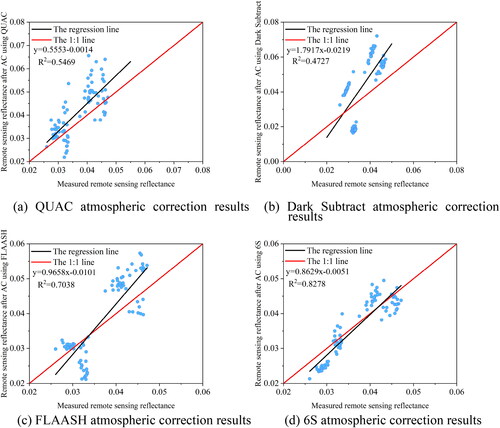
Based on Zhuhai-1 hyperspectral images, four types of approaches (QUAC, Dark Subtract, FLAASH and 6S) are utilized to undertaken AC. The results obtained and synchronously measured spectral data are comparatively analyzed. The AC results from different approaches are shown in Figure 4, the number of sampling points is 20, and the band is selected as B1∼B32.

Figure 4. Scatter plots of remote sensing reflectance data after AC and reflectance of measured data.

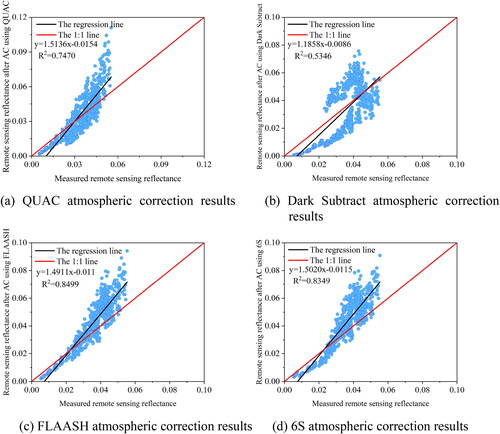
As shown in Figure 4, the reflectance range after AC using QUAC, Dark Subtract, FLAASH, and 6S is 0 to 0.12. In the range from 0 to 0.03, the reflectance corrected using these methods is low overall compared with measured reflectance; between 0.03 and 0.12, the reflectance after AC using these methods is high compared with measured data. Among which, Dark Subtract has the poorest correction accuracy, as illustrated in Figure 4(b): $R^2$ is 0.5346 and the reflectance after AC using Dark Subtract ranges from 0 to 0.08. As presented in Figure 4(a), QUAC exhibits a correction accuracy slightly higher than that of Dark Subtract: $R^2$ is 0.7470 and the reflectance corrected using QUAC ranges from 0 to 0.12. As shown in Figure 4(c), FLAASH has the highest correction accuracy among the four models: $R^2$ is 0.8499, the reflectance corrected using FLAASH ranges from 0 to 0.10; 6S with $R^2$ of 0.8349 showing a correction accuracy marginally lower than that of FLAASH, the reflectance corrected using 6S ranges from 0 to 0.10, as shown in Figure 4(d).

4.1.2. Comparative analysis of single-band AC accuracy

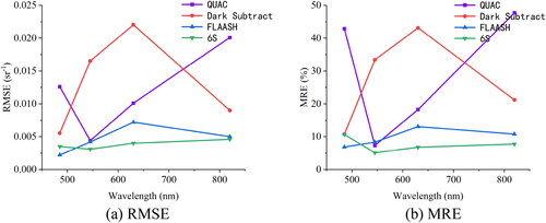
Based on measure spectra, the RMSE and MRE of different wave bands for all sampling points of the Zhuhai-1 images after AC are calculated, as shown in Figure 4.

For single wave bands, as shown in Figure 5(a), in the range of 466–566 nm, Dark Subtract, FLAASH and 6S show similar rising trends in RMSE, reaching a maximum value at 566 nm; QUAC shows the opposite trend, reaching a minimum value at 566 nm. From 566 to 700 nm, the RMSE of QUAC increases; the RMSE of Dark Subtract, FLAASH, and 6S show a declining trend between 566 and 640 nm, a rising trend from 640 to 700 nm, reaching a maximum value at 700 nm; from 700 to 940 nm, the RMSE of four methods exhibit a decreasing trend.

Figure 5. Accuracy comparison of each band after AC.

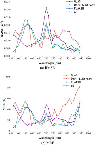
As shown in Figure 5, QUAC returns a higher accuracy in the NIR band at B26-B29 (850–896 nm), while the RMSE is between 0.005–0.0075 and MRE is below 18%, which is applied to the model for inversion of water body imagery data in this region using NIR bands. Dark Subtract has a higher accuracy in the red bands at B9-B14 (596–670 nm), with RMSE ranging between 0.005 and 0.015 and an RME of less than 19%. This is suitable for use in the model for inversion of water body data in this region using red bands; FLAASH has a higher accuracy in the red and NIR bands at B19-B28 (746–880 nm), with an RMSE between 0.0025–0.01 and an MRE below 25%. It is applicable to the model for inversion of water body in this region using red and NIR bands. 6S presents a higher accuracy in red and NIR bands at B19-B26 (746–850 nm), with an RMSE ranging from 0.0025 to 0.01 and an MRE below 20%, making it suitable for use in the model for inversion of such data in this region using red and NIR bands.

4.2. AC results and analysis based on Sentinel-2 satellite data

4.2.1. Overall performance of comparative analysis

Based on Sentinel-2 images, QUAC, Dark Subtract, FLAASH and 6S are used for AC. The AC results and synchronously measured spectral data are comparatively analyzed. The AC results of each method are illustrated in Figure 6, the number of sampling points is 20, and the band is selected as B2∼B8A.

Figure 6. Remote sensing data reflectance after AC and the reflectance of measured data.

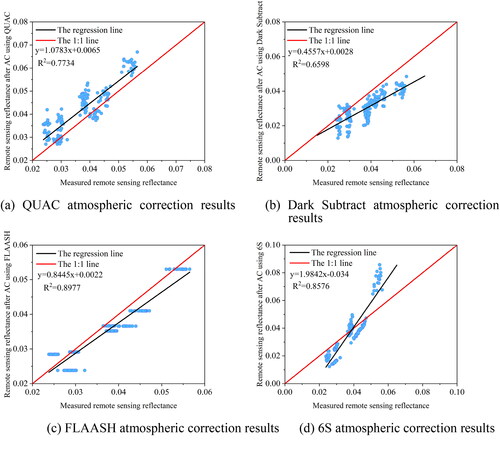
As can be seen from Figure 6, Dark Subtract returns the poorest AC accuracy among the four methods (QUAC, Dark Subtract, FLAASH, and 6S); as shown in Figure 6(b), $R^2$ is 0.6598 and the reflectance ranges from 0.001 to 0.05 after correction and is generally lower than the measured reflectance. The AC accuracy of QUAC, as presented in Figure 6(a), slightly outperforms that of Dark Subtract, $R^2$ is 0.7734 and the corrected reflectance ranges between 0.02 and 0.07 being generally higher than the measured reflectance. Among the four methods, FLAASH returns the highest accuracy as shown in Figure 6(c) with $R^2$ = 0.8977, the reflectance (when corrected) ranges from 0.02 to 0.06, the corrected reflectance is generally lower than the measured reflectance. The 6S method (with $R^2$ = 0.8576, as shown in Figure 6(d)), returns an accuracy slightly lower than that of FLAASH; the corrected reflectance corrected ranges from 0.01 to 0.10; when the reflectance is between 0.01 and 0.03, the corrected reflectance is generally lower than the measured reflectance; in the range from 0.03 to 0.10, the corrected reflectance is higher than the measured reflectance.

4.2.2. Comparative analysis of single band accuracy

Based on measured spectra, the RMSE and MRE of each band for all sampling points of Sentinel-2 images after AC using four methods are calculated, with the results shown in Figure 7.

Figure 7. Accuracy comparison of each band after AC.

For a single band, as shown in Figure 7(a), the overall performance of FLAASH is best, with an RMSE of around 0.005, the overall change is stable and the RMSE is the smallest at 842 nm. QUAC and Dark Subtract show similar changes in RMSE; at 490–705 nm, RMSE presents a rising trend; while at 740–842 nm, RMSE tends to decline. The 6S method shows the poorest performance at 705 nm and its RMSE is the highest among the four methods. The method presents better performance at other wave-band ranges.

Figure 7 shows that QUAC presents a higher accuracy at B2 blue (490 nm) and B3 green (560 nm) bands with RMSE ranging between 0.001–0.003 and MRE lower than 5%, making it suitable for use in the model for inversion of water body data in this region using blue and red bands; Dark Subtract shows a higher accuracy at B2 blue (490 nm) and B8A NIR (865 nm) bands, with RMSE ranging from 0.001 to 0.007 and MRE lower than 22%, making it suitable for use in the model for inversion of water body data in this region using blue and NIR bands; FLAASH demonstrates a larger accuracy at the B5 vegetation red edge (705 nm) and B8 NIR (842 nm) bands, with RMSE of 0.0005–0.002 and MRE below 3%, making it suitable for use in the model for inversion of water body data in this region utilizing vegetation red edge and NIR bands; the 6S method indicates a higher accuracy at B4 red (665 nm) and B6 vegetation red edge (740 nm) bands, having an RMSE of 0.003–0.004 and MRE lower than 8%. It can be applied in the model for inversion of water body data in this region using red and vegetation red edge bands.

4.3. AC results and analysis based on planet satellite data

4.3.1. Comparative analysis of overall performance

The AC was conducted using QUAC, Dark Subtract, FLAASH and 6S based on Planet images. AC results obtained and synchronously measured spectral data are comparatively analyzed undertaken, with the AC results obtained using each method as shown in Figure 8, the number of sampling points is 20, and the band is selected as B1∼B4.

Figure 8. Remote sensing reflectance after AC and reflectance of measured data.

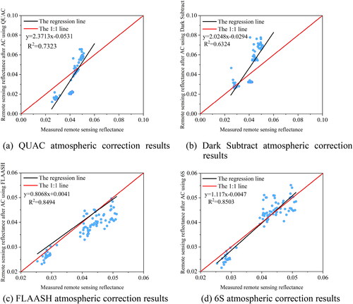
As shown in Figure 8, Dark Subtract, among the four methods (QUAC, Dark Subtract, FLAASH, and 6S), returns the poorest AC accuracy (Figure 8b): $R^2$ is 0.6324 and the corrected reflectance is between 0.02 and 0.08, generally exceeding that measured. The AC accuracy of QUAC (Figure 8a) is slightly higher than that of Dark Subtract: $R^2$ is 0.7323 and the corrected reflectance ranges from 0.01 to 0.07; in the range of 0.01 to 0.04, the corrected reflectance is lower than that measured; in the range from 0.04 to 0.07, the corrected reflectance exceeds that measured. The AC accuracies of FLAASH and 6S (Figures 7c and 6) are similar; among the four methods, 6S (Figure 8d) returns the highest AC accuracy: $R^2$ is 0.8503 and the corrected reflectance ranges from 0.02 to 0.06; in the range from 0.02 to 0.03, the corrected reflectance is smaller than that measured; in the range from 0.03 to 0.06, the corrected reflectance exceeds that measured. The AC accuracy of FLAASH (Figure 8c) is marginally inferior to that of 6S: $R^2$ is 0.8494 and the corrected reflectance ranges from 0.02 to 0.06: in the range from 0.02 to 0.035, the corrected reflectance exceeds that measured; the corrected reflectance in the range from 0.035 to 0.06 is uniformly distributed on both sides of the 1:1 line.

4.3.2. Comparative analysis of single band accuracy

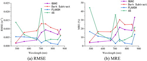
The RMSE and MRE of each band for all sampling points of Planet images subjected to AC are calculated based on measured spectra, with the results as shown in Figure 9.

Figure 9. Accuracy comparison of each band after AC using different methods.

As presented in Figure 9a, for single band, 6S shows the best overall performance. The RMSE of different bands are below 0.005, indicating that the overall change is stable. The RMSE at 545 nm are the smallest. The root mean square error variation of the FLAASH method is close to that of 6S, with the RMSE reaching the minimum at 485 nm. QUAC and Dark Subtract exhibit a large change in terms of single bands. Their overall performance is poorest, with RMSE reaching the minimum at 545 nm and 485 nm.

As shown in Figure 9, QUAC demonstrates a higher accuracy at B2 green (545 nm) and B3 red (630 nm) bands, with RMSE ranging between 0.004–0.015 and MRE below 20%. The model can be applied for the inversion of water body data in this region utilizing green and red bands. Dark Subtract returns a higher accuracy at B1 blue (485 nm) and B4 near-infrared (820 nm) bands, with RMSE ranging from 0.005 to 0.01 and MRE lower than 25%. It can be applied in the inversion of water body data in this region using blue and near-infrared bands. FLAASH returns a higher accuracy at B1 blue (485 nm) and B2 green (545 nm), with RMSE ranging between 0.002–0.005 and MRE below 10%, making it suitable for use in the inversion of water body data in this region using blue and green bands. 6S demonstrates a higher accuracy at B2 green (545 nm) and B3 red (630 nm) bands, with RMSE ranging between 0.003–0.005 and MRE below 10%. The model can be applied for the inversion of water body data in this region utilizing green and red bands.

4.4. AC results and analysis based on GF-2 satellite data

4.4.1. Comparative analysis of overall performance

Based on GF-2 images, QUAC, Dark Subtract, FLAASH, and 6S are used for AC. The comparative analysis of AC results obtained and synchronously measured spectral data was carried out. The AC results for different methods are shown in Figure 10, the number of sampling points is 20, and the band is selected as B1∼B4.

Figure 10. Remote sensing data reflectance after AC and reflectance of measured data.

As shown in Figure 10, among the four methods (QUAC, Dark Subtract, FLAASH and 6S), Dark Subtract shows poorest AC accuracy as presented in Figure 10(b), $R^2$ is 0.4727 and the corrected reflectance ranges from 0.01 to 0.08; between 0.01 and 0.03, the corrected reflectance is generally lower than that measured. The accuracy of QUAC is slightly superior to Dark Subtract: $R^2$ is 0.5469 and the corrected reflectance is generally higher than that measured, within the range of 0.02 to 0.0.7. The 6S method (Figure 10d) returns the highest AC accuracy among the four models: $R^2$ is 0.8278 and the corrected reflectance ranges from 0.02 to 0.05; in the range from 0.02 to 0.03, the corrected reflectance is compared with that measured, which is generally low. In the range from 0.03 to 0.04, the corrected reflectance is generally higher than that measured; in the range from 0.04 to 0.05, the corrected reflectance is relatively uniformly distributed on each side of the 1:1 line. FLAASH has a correction accuracy slightly inferior to that of 6S and $R^2$ is 0.7038, as presented in Figure 10c: the corrected reflectance ranges from 0.02 to 0.06: in the ranges from 0.02 to 0.025 and 0.035 to 0.045, the corrected reflectance is generally smaller than that measured; in the ranges from 0.025 to 0.035 and 0.045 to 0.06, relative to measured reflectance, the corrected reflectance is higher.

4.4.2. Comparative analysis of single band accuracy

Based on measured spectra, the RMSE and MRE of each band for all sampling points from GF-2 images after AC are calculated, as presented in Figure 11.

Figure 11. Accuracy comparison of each band after AC using different methods.

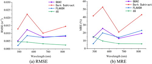
As illustrated by Figure 11 (a), the overall performance of 6S for single band is the best. The RMSE of each band is lower than 0.005; its overall change is quite stable, reaching the lowest at around 821 nm. The RMSE of QUAC, Dark Subtract, and FLAASH demonstrate a similar trend. In the range of 491–555 nm, the RMSE of the three methods all present a rising trend; in the case of 555- 665 nm, RMSE exhibit a declining trend; at 665–821 nm, the RMSE of the three methods all show an increasing trend.

As shown in Figure 11, QUAC has a higher accuracy at B1 blue at 491 nm and B3 red bands at 665 nm, with RMSE ranging from 0.005 to 0.01 and MRE lower than 15%, which suits the inversion model of water body in this region that utilizes blue and red bands. Dark Subtract demonstrates a greater accuracy at B1 blue (491 nm) and B3 red (665 nm) bands, with RMSE ranging between 0.01–0.015 and MRE below 45%, making it suitable for use in the inversion model of water body data in this region using blue and red bands. FLAASH exhibits a higher accuracy at B1 blue (491 nm) and B3 red bands (665 nm), with RMSE ranging from 0.002 to 0.01 and MRE lower than 15%. It can be applied in the inversion of water body data in this region using blue and red bands. 6S has a higher accuracy at B3 red (665 nm) and B4 NIR (821 nm) bands, with RMSE ranging from 0.002 to 0.05 and MRE lower than 10%, making it suitable for use in the inversion of water body data in this region using red and NIR bands.

4.5. Comparison and analysis of AC results

The coefficient of determination and MRE after AC on four types of satellite data are summarized in Table 1. The comparative analysis shows that: after conducting AC on four types of images (Zhuhai-1, Sentinel-2, Planet, and GF-2), FLAASH and 6S methods are superior to QUAC and Dark Subtract, indicating FLAASH and 6S are more applicable to lake water color remote sensing data inversion, this conclusion is consistent with the study (Du et al. 2014; Li et al. 2021). Judging from analysis of AC methods and satellite images, QUAC and Dark Subtract as empirical, statistics-based methods are mainly based on measured data and a priori knowledge, showing strong subjectivity and difficult to reflect real spectral features of surface objects after AC; while the FLAASH and 6S methods based on radiative transfer models set appropriate atmospheric parameters using radiative transfer models the more rationally to reflect radiance absorption and scattering processes in the atmospheric radiative transfer process, consequently obtaining more real image AC reflectance data. For Planet and GF-2 multispectral images, 6S is superior to FLAASH; while for multispectral Sentinel-2 images and hyperspectral Zhuhai-1 images, FLAASH outperforms 6S, this is possibly because the model parameters of 6S method are relatively complicated, and some parameters are difficult to obtain accurately, resulting in the inferior correction accuracy of the FLAASH method.

Table 1. Comparison of AC results from four types of satellite data.

		Zhuhai-1	Sentinel-2	Planet	GF-2
R^2	QUAC	0.7470	0.7734	0.8385	0.5469
	Dark Subtract	0.5346	0.6598	0.6324	0.4727
	FLAASH	0.8499	0.8977	0.8494	0.7038
	6S	0.8349	0.8576	0.8503	0.8278
RMSE	QUAC	0.0120	0.0068	0.0128	0.0085
	Dark Subtract	0.0131	0.0093	0.0145	0.0151
	FLAASH	0.0110	0.0036	0.0049	0.0070
	6S	0.0113	0.0098	0.0038	0.0037
MRE	QUAC	24.75%	14.93%	29.05%	18.07%
	Dark Subtract	38.33%	19.67%	27.11%	39.62%
	FLAASH	21.51%	8.32%	9.76%	15.86%
	6S	23.89%	18.47%	7.57%	9.29%

5. Conclusion

This research respectively used QUAC, Dark Subtract, FLAASH, and 6S methods to conduct AC on Zhuhai-1, Sentinel-2, Planet, and GF-2 images of the Tiande Lake zone, Zhengzhou, China. The results obtained are compared with water surface spectral data measured using a ground object spectrometer. The following conclusions can be drawn:

1. For Zhuhai-1 and Sentinel-2 images, the overall performance of FLAASH is better when the coefficients of determination $R^2$ are 0.8499 and 0.8977, RMSE are 0.0110 and 0.0036, and MRE are 21.51% and 8.32% respectively. Aiming at Planet and GF-2 images, 6S shows better overall performance among the four methods; $R^2$ values are 0.8503 and 0.8278 respectively, RMSE are 0.0038 and 0.0037, and MRE are 7.57% and 9.29% separately. Through single-band accuracy comparative analysis, it is preliminarily concluded that four atmospheric correction methods are suitable for constructing sensitive bands of water quality inversion models in different images

2. Comparison of AC results for four types of images shows that FLAASH and 6S present better applicability; their overall performances are superior to those of QUAC and Dark Subtract. The discrepancies in the results are lower, indicating that FLAASH and 6S are more applicable to lake water color remote sensing data inversion

Disclosure statement

No potential conflict of interest was reported by the author(s).

Additional information

Funding

This work was supported by the Science and Technology Public Relations Project of Henan Province (Grant no. 232102320123).

References

- Adler-Golden SM, Matthew MW, Bernstein LS, et al. 1999. Atmospheric correction for shortwave spectral imagery based on MODTRAN4[C]. Imag Spectrom V SPIE. 3753:61–69.
- Bernardo N, Watanabe F, Rodrigues T, Alcântara E. 2017. Atmospheric correction issues for retrieving total suspended matter concentrations in inland waters using OLI/Landsat-8 image. Adv Space Res. 59(9):2335–2348. doi: 10.1016/j.asr.2017.02.017.
- Bernstein LS, Jin X, Gregor B, et al. 2012. Quick atmospheric correction code: algorithm description and recent upgrades. Opt Eng. 51(11):111719–111719. doi: 10.1117/1.OE.51.11.111719.
- Cai L, Bu J, Tang D, Zhou M, Yao R, Huang S. 2020. Geosynchronous satellite GF-4 observations of Chlorophyll-a distribution details in the Bohai Sea, China. Sensors. 20(19):5471. doi: 10.3390/s20195471.
- Cheng CM, Wei YC, Li Y, Tu QG. 2020. The 6S image-by-image atmospheric correction of GF-1/WFV images of Taihu Lake water bodies. Remote Sens Technol Appl. 35(01):141–152.
- Ding F. 2018. Comparison and suitability evaluation of Taihu OLI images [D]. Shaanxi:Xi’an University of Science and Technology.
- Doxani G, Vermote EF, Roger J-C, Skakun S, Gascon F, Collison A, De Keukelaere L, Desjardins C, Frantz D, Hagolle O, et al. 2023. Atmospheric Correction Inter-comparison eXercise, ACIX-II Land: an assessment of atmospheric correction processors for Landsat 8 and Sentinel-2 over land. Remote Sens Environ. 285:113412. doi: 10.1016/j.rse.2022.113412.
- Du T, Wang XH, Liang HY, et al. 2014. Comparative study on atmospheric correction model of lake chlorophyll A inversion. J Yun Univ (Nat Sci Ed). 36(02):241–248.
- Duan HT, Cao ZG, Shen M, Ma JG, Qi TC. 2022. Research progress and prospect of lake remote sensing research. J Rem Sens. 26(01):3–18.
- Guan H, Huang J, Li X, Zeng Y, Su W, Ma Y, Dong J, Niu Q, Wang W. 2022. An improved approach to estimating crop lodging percentage with Sentinel-2 imagery using machine learning. Int J Appl Earth Obs Geoinf. 113:102992. doi: 10.1016/j.jag.2022.102992.
- Guo YK, Zeng F. 2012. Comparison of atmospheric correction of SPOT 5 images based on FLAASH and QUAC model. Survey Mapp Bul. 11:21–23.
- Hou XZ, Yi WN, Qiao YL, Huang HL, Cui WY, Du LL, Chen C. 2015. Atmospheric Correction Method for Remote Sensing Image Based on 6S Model. J Atmos Environ Optics. 10(01):63–68.
- Hu Y, Liu L, Liu L, Peng D, Jiao Q, Zhang H. 2014. A landsat-5 atmospheric correction based on MODIS atmosphere products and 6S model. IEEE J Sel Top Appl Earth Observ Rem Sens. 7(5):1609–1615. doi: 10.1109/JSTARS.2013.2290028.
- Kaufman YJ, Sendra C. 1988. Algorithm for automatic atmospheric corrections to visible and near-IR satellite imagery. Int J Remote Sens. 9(8):1357–1381. doi: 10.1080/01431168808954942.
- Lantzanakis G, Mitraka Z, Chrysoulakis N. 2017. Comparison of physically and image based atmospheric correction methods for Sentinel-2 satellite imagery[M]. Perspectives on atmospheric sciences. Cham: Springer; p. 255–261.
- Li ZQ, Chen XF, Ma LY, et al. 2018. Review of atmospheric correction of optical remote sensing satellites. J Nanjing Univ Inform Scie Technol (Nat Sci Ed). 10(01):6–15.
- Li HC, Kuang RY, Song ZH. 2021. Evaluation of poyang lake atmospheric correction method based on sentinel-2 image. Space Ret Rem Sens. 42(04):108–119.
- Liu G, Li Y, Lyu H, Wang S, Du C, Huang C. 2016. An improved land target-based atmospheric correction method for Lake Taihu. IEEE J Sel Top Appl Earth Observ Rem Sens. 9(2):793–803. doi: 10.1109/JSTARS.2015.2503800.
- Luo K, Wei Y, Du J, Liu L, Luo X, Shi Y, Pei X, Lei N, Song C, Li J, et al. 2022. Machine learning-based estimates of aboveground biomass of subalpine forests using Landsat 8 OLI and Sentinel-2B images in the Jiuzhaigou National Nature Reserve, Eastern Tibet Plateau. J Res. 33(4):1329–1340. doi: 10.1007/s11676-021-01421-w.
- Martins V, Barbosa C, de Carvalho L, Jorge D, Lobo F, Novo E. 2017. Assessment of atmospheric correction methods for Sentinel-2 MSI images applied to Amazon floodplain lakes. Rem Sens. 9(4):322. doi: 10.3390/rs9040322.
- Mu C, Liu ZY, Meng D. 2021. Atmospheric correction of inland lake water bodies based on Sentinel-2 satellite data. Survey Map Bul. 09:9–14.
- Pan Y, Bélanger S, Huot Y. 2022. Evaluation of atmospheric correction algorithms over lakes for high-resolution multispectralimagery: implications of adjacency effect. Rem Sens. 14(13):2979. doi: 10.3390/rs14132979.
- Tian QL, Qin K, Chen XJ, Yu CF. 2021. Comparative study of the atmospheric correction method for WorldView-3 satellite images. World Nuclear Geol Sci. 38(02):229–236.
- Vermote EF,Tanre D,Deuze JL,Herman M,Morcette J-J. 1997. Second Simulation of the Satellite Signal in the Solar Spectrum, 6S: an overview. IEEE Trans Geosci Remote Sensing. 35(3):675–686. doi: 10.1109/36.581987.
- Wang SM, Dou HS. 1998. The lake annals of China [M]. Beijing: Science Press.
- Wang D, Ma R, Xue K, Loiselle S. 2019. The assessment of Landsat-8 OLI atmospheric correction algorithms for inland waters. Remote Sens. 11(2):169. doi: 10.3390/rs11020169.
- Xie EH, Wu JE, Yang K. 2022. Inversion of chlorophyll A mass concentration in Erhai Lake based on Sentinel-2 images. J Environ Eng. 16(9):3058–3069.
- Zheng W, Zeng ZY. 2004. Review of atmospheric correction methods of remote sensing images. Rem Sens Inform. 19(04):66–70.