A landscape metrics-based sample weighting approach for forecasting land cover change with deep learning models

Abstract

Unaddressed imbalance of multitemporal land cover (LC) data reduces deep learning (DL) model usefulness to forecast changes. To manage geospatial data imbalance, there is a lack of specialized cost-sensitive learning strategies available. Sample weights are typically derived from training instance frequencies which disregard spatial pattern complexities. Therefore, this study proposes a geospatial sample weighting approach underpinned by class-level landscape metrics (LSMs) to assign importance to categories based on relative indicators of spatial form. A case study demonstrates the application and effects of the LSM-based sample weighting approach for projecting LC changes of a region in British Columbia, Canada. Four spatiotemporal DL models are provided weighted training samples including multitemporal LC data and explanatory factors. Sample weights calculated from indicators of patch density, shape irregularity and shape heterogeneity improved figure of merit and related measures over baseline configurations. This study contributes to LC change data imbalance management strategies for DL models.

Keywords:

• Land cover change
• landscape metrics
• geographic data imbalance
• sample weights
• spatiotemporal deep learning

1. Introduction

Land change is of great significance to a vast array of environmental systems, with human-induced changes spurring natural disasters, biodiversity loss, and exposure to new diseases (Turner et al. 2007). Previously, land change models were implemented with statistical techniques, expert-encoded knowledge systems, and geographic automata (Parker et al. 2003). Researchers also demonstrated the potential of hybrid models that integrated longstanding approaches like cellular models with Markov chains (Yang et al. 2014), neural networks (NNs) (Li and Yeh 2002), and deep NNs (Xing et al. 2020). With increasing amounts of geospatial data available, machine learning (ML) and deep learning (DL) techniques are gaining attention for extrapolating patterns from historical land change datasets and to bypass manual specification of transition rules (Ren et al. 2019; Harati et al. 2020). Data-driven components can then be used to automate projections of future land changes and to enhance other model types.

Recently, land change studies have increasingly benefitted from expanding availability of multitemporal remotely sensed (RS) data products, shifting modelling endeavours away from decadal toward annual and even real-time analyses (Zhu et al. 2022). While advancements of DL methodologies have enabled studies to leverage these datasets (Zhang et al. 2022), using DL for land cover (LC) change forecasting applications remains a nascent research area (Wang et al. 2022). An open problem hindering adoption of DL models for LC change forecasting stems from two primary dimensions of imbalance inherent to multitemporal LC datasets (Karpatne et al. 2016). First, DL models demonstrate biases toward majority classes because internal parameters are influenced equally by each sample during model training procedures (Johnson and Khoshgoftaar 2019; Zhang and Li 2022). Next, the effects of limited change events in training datasets worsen biases. These properties simultaneously diminish DL model performance, leading to overly complicated models with seemingly poor LC change forecasting capacity when the problem is unaddressed (van Duynhoven and Dragićević 2022b). Therefore, addressing DL model sensitivities to imbalanced geographic data is crucial for developing data-driven LC models which can concurrently use the vast amounts of data available and successfully project changes across multiple classes.

To manage dimensions of the imbalance problem, earlier research studies have used data-level manipulations including synthetic data augmentation (Sefrin et al. 2020), oversampling (Wang et al. 2019), and undersampling (van Duynhoven and Dragićević 2019). Yet, widely used data augmentation techniques like rotating and flipping remotely sensed image samples are unsuitable for geographic data samples because they abandon spatial directional relationships (Zhu et al. 2019). Oversampling techniques also intensify the risk of overfitting because of overrepresentation of certain areas and spatial structures (Kellenberger et al. 2018; Zhang et al. 2022). On the other hand, undersampling schemes may omit important samples (Tarawneh et al. 2022) and undercut the data-intensive needs of DL models (Nikparvar and Thill 2021). As an alternative, algorithm-level techniques like cost-sensitive learning (He and Garcia 2009) avoid dataset manipulations which add detrimental synthetic samples or remove important observations (Johnson and Khoshgoftaar 2019). Cost-sensitive learning involves allotting penalties to each sample based on its relative importance in the training dataset, where higher penalties actuate greater magnitudes of change to a model’s learned parameters (Lu et al. 2022). Class weights (CWs) or sample weights (SWs) can be assigned manually (Kang et al. 2022), by systematic exploration of penalties (Zhang et al. 2022), using probabilities of occurrence (Van den Broeck et al. 2022), or dynamically during model training with respect to sample difficulty (Zhang et al. 2022).

Popular CW schemes are derived from per-class sample counts. These include variations of inverse frequency weighting (IFW) (Yan et al. 2022) and effective number weighting (ENW) (Cui et al. 2019). The IFW scheme operates by assigning CWs inversely proportional to the number of samples belonging to each category in a dataset (Zhong et al. 2019). Previous studies employed IFW schemes to ensure LC classes comprising smaller proportions of the landscape were allocated higher importance than dominant LC types (Zhong et al. 2019; Sefrin et al. 2020). Assuming that most samples of the same class exhibit similarities, the ENW scheme was also devised to calculate the ‘effective number’ of samples for each class (Cui et al. 2019). Recent RS studies have used ENW in a methodology implemented to detect sparser forest structures (Brandt and Stolle 2021). Currently, CW schemes derived from inverting class frequencies or areas is the de facto strategy built into popular geographic information systems (GIS) software like ArcGIS Pro’s ‘Class Balancing’ setting for training DL models (Esri 2023) and open-source library functions like scikit-learn’s ‘Compute Class Weight’ function (Pedregosa et al. 2011). However, obtaining relative importance from sample quantities neglects the characteristics of geographic data and various idiosyncrasies of LC data. For instance, CW schemes derived from class frequencies are problematic for LC change models because classes covering relatively small areas are not always guaranteed to be active or expanding. In addition, per-class frequencies disregard complexities of the spatial structure and arrangement of each LC type. With longstanding class-level landscape metrics (LSMs) available to quantify landscape configurations (Frazier and Kedron 2017), substituting frequency-based schemes for spatial pattern indicators could instead retain the relative significance of each LC type based on their spatial form. LSMs are useful indicators of the conditions, activities, and influences driving landscape changes (Amiri et al. 2017), but developing cost-sensitive learning strategies from spatial pattern measures is unexplored.

At present, there is a lack of specialized cost-sensitive learning techniques available for geographic data. The primary goal of this study is to propose and evaluate a new LSM-based sample weighting strategy for managing geographic data imbalance and improving data-driven model effectiveness in forecasting multi-class LC changes. Specifically, the procedure leverages class-level LSMs to summarize the spatial configuration of patches belonging to each category. The proposed sample weighting approach aims to help integrate knowledge about the composition of an area in mitigating geographic data imbalance without needing to manually manipulate the dataset, adjust SW settings by hand, or rely on aspatial SW derivation techniques that do not reflect the properties of geographic data.

The presented strategy includes four steps to analyze and interpret the key indicators of spatial pattern of a study area, to capture the relative significance of spatial structure for each LC class, to manage model biases toward persistent areas, and to calculate combined SWs which manage the principal dimensions of LC data imbalance. To demonstrate the application and effects of the proposed LSM-based sample weighting framework, a case study is shown for modelling LC changes of the Tumbler Ridge District Municipality of British Columbia, Canada. A small set of class-level LSMs related to this region are selected to derive SWs for use in training four spatiotemporal DL model types, including CNN-LSTM, CNN-GRU, CNN-TCN, and Convolutional LSTM (ConvLSTM). The purpose of assessing the effects of the LSM-based sample weighting strategy across model types is to uncover any consistent behaviours emerging regardless of model architecture variations. Each configuration was used to project LC changes for five years in the presence of severely imbalanced LC classes and small amounts of change. The overall and per-class LC changes outputted by the models trained with the specialized SWs are compared to those trained with conventional frequency-based weighting schemes. The goal is to determine the efficacy of a specialized spatial sample weighting schemes designed for the idiosyncrasies of imbalanced geospatial data.

2. Methodology

2.1. Study area and datasets

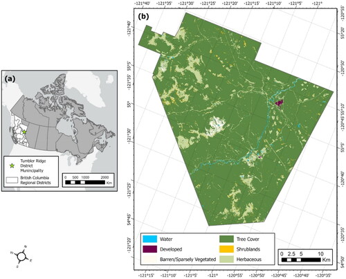
The area selected for the case study is the Tumbler Ridge District Municipality, located in the Peace River region of British Columbia, Canada (Figure 1a and b). Mining, forestry, and alternative energy industries are primary drivers of this rural region’s economy, sustaining a local population of 2399 as of 2021 (Statistics Canada 2023). Endeavours to diversify the resource-dependent economy have also included establishing a paleontology research center, a UNESCO Geopark site, and tourism initiatives (Halseth et al. 2017; Ryser et al. 2019). This study area was selected for several reasons. First, the number of timesteps and annual temporal resolution of the geographic data available for this region is sufficient for training the DL models, as per recommendations of previous studies (van Duynhoven and Dragićević 2019). Next, the severe imbalance of LC types for this area is guaranteed to inhibit meaningful models to be learned without any data imbalance mitigation strategies. Lastly, a more rural area was used to exemplify the LSM-based sample weighting scheme to reduce the interplay of anthropogenic factors. For example, there are no protected areas or agricultural land reserves explicitly in this region. It is acknowledged that human activities and policies may be better represented by different types of models or hybrid implementations. However, since the intention of the case study is to exemplify the setup and effects of the proposed SW framework on a data-driven LC change model, the focus is not to devise a “perfect” model for the region.

Figure 1. Study area details showing (a) the Tumbler Ridge District Municipality in British Columbia, Canada, and (b) the 2001 LC of the study area displayed using the Canada Lambert conformal conic projected coordinate system.

2.1.1. Multitemporal LC data

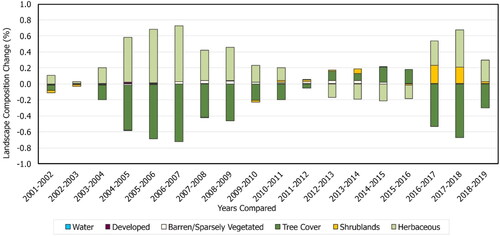
The LC information for the municipality is obtained from the Global Land Cover Mapping and Estimation (GLanCE) data product (Arevalo et al. 2022). The GLanCE data source provides annual LC data at 30-mr spatial resolution for years 2001 through 2019, which is realigned to the NAD 1983 UTM Zone 10N projected coordinate system for this study. The 30-m spatial resolution provides an appropriate level of detail to differentiate settlements, forests and types of vegetation (Martínez and Mollicone 2012) and for modelling land changes (Yang et al. 2014). All datasets used were processed to maintain these properties. The LC categories used in this study include water, developed, barren or sparsely vegetated (areas covered by less than 10% vegetation), tree cover (land with tree coverage of 30% or more), shrublands (land with tree coverage less than 30%) and herbaceous (areas covered by less than 30% trees and less than 10% shrubs). The types of LC characterizing Tumbler Ridge are imbalanced (Figure 2), with tree cover comprising 87% of the study area in 2001 and decreasing by approximately 5% by 2019. The inequality of changed versus persistent areas is apparent when analyzing the gaining and losing LC types of the region (Figure 3). The largest total annual LC change occurred between 2006 and 2007, affecting less than 1% of the study area. It should also be noted that reported issues within the GLanCE data product stem from difficulties differentiating shrublands and herbaceous LC types, predominantly in high latitudes and arid locations (Friedl et al. 2022). While the Tumbler Ridge region does not qualify as either affected area, the lower overall classification accuracies reported for these LC classes is still expected to impact data-driven model performance.

Figure 2. A comparison of the landscape composition in years 2001 and 2019 expressed as a percentage of the landscape.

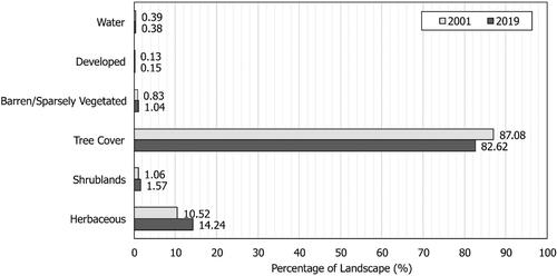
Figure 3. The percentage of annually changed landscape area with respect to each LC class from 2001 to 2019.

2.1.2. Auxiliary spatial variables

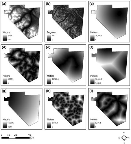
Alongside the multitemporal GLanCE data, additional explanatory factors of land change are provided as constant spatial datasets (Figure 4). Spatial variables pertaining to topography include elevation and slope (Pickard et al. 2017) are drawn from the ASTER global digital elevation model (Abrams et al. 2015). Additional variables related to accessibility were derived to represent the Euclidean distance to population centres (Aguejdad et al. 2017), roads (Mungai et al. 2022), railways (Xing et al. 2020), parks and protected areas (Ye et al. 2019), agricultural land reserves (Yaghoobi et al. 2022), lakes (Machemer et al. 2006), and rivers (Asempah et al. 2021). Features necessary to compute each variable were obtained from Statistics Canada and the British Columbia Data Catalogue.

Figure 4. Auxiliary spatial variables prior to Min-max normalization and displayed using the NAD 1983 UTM 10N projected coordinate system: (a) elevation, (b) slope, (c, d) distance to population centres, (e) distance to roads, (f) distance to parks and protected areas, (g) distance to agricultural land reserves, (h) distance to lakes, and (i) distance to rivers.

2.1.3. Preparing training data samples

Preparing the training, validation and testing data samples involves extracting the neighbouring features of every cell over all timesteps. The surroundings of each location are important to consider because of neighbourhood effects, where nearby states influence the central cell (Xing et al. 2020). Spatiotemporal LC is obtained for the $M\times M$ neighbourhood surrounding each cell $i$ at each timestep $T,$ where $M$ indicates the length of the longest edge of the cell’s neighbourhood. Another dimension for storing binarized or ‘one-hot-encodings’ to represent to LC categories is added (Jagannathan and Divya 2021), where the number of possible LC categories denoted by $L.$ Thus, each sample’s spatiotemporal LC data component retains the dimensions $T\times M\times M\times L.$ Additionally, the auxiliary spatial variables associated with each cell $i$ maintain the dimensions $M\times M\times A,$ where $A$ denotes the number of explanatory variables prepared for the study region.

Based on previous studies (Masolele et al. 2021; van Duynhoven and Dragićević 2022a) using 30-m spatial resolution data, the neighbourhood dimension is set to $M$ = 9. The edge effects in this study are managed by allowing samples to contain neighbours outside of the study area boundary (Fotheringham and Rogerson 1993). A buffer zone of four cells or 1.2 km in each direction from the study area boundary is included, ensuring that neighbourhoods of locations near to the study area boundaries contain meaningful values instead of nulls or zeroes. The LC category dimension is set as $L=7$ to accommodate the possibility of no LC types assigned to a cell. Lastly, the number of explanatory variables is indicated as $A=9.$

Experimental datasets are derived by obtaining subsets from the LC data available from 2001 to 2019. To ensure sufficient sequence lengths for training, validation and testing datasets, the number of timesteps $T$ is set to 12. Input datasets are derived following a ‘rolling window’ procedure (Xiao et al. 2019), which increments the sequence by one year at a time. Accordingly, the LC included in the training dataset spans 2001 to 2013, where 2013 provides the training data label and 2001 to 2012 supply the inputted training data sequence. The validation data spans 2002 to 2013, where the validation label corresponds to the 2014 LC. The first sequence comprising the testing dataset covers 2003 to 2014, with the models used to project the real-world LC data for 2015, 2016, 2017, 2018, and 2019. This means that the model’s forecast of 2015 supplies the next timestep of the input sequence to project the 2016 LC and so on.

2.2. DL model implementation

Four spatiotemporal DL models were chosen to explore consistency of weighting scheme effects across different model architectures. The models selected were CNN-LSTM, CNN-GRU, CNN-TCN, and Convolutional LSTM (ConvLSTM). The model architectures integrate convolutional neural networks (CNNs) (LeCun et al. 2015) with long short-term memory networks (LSTMs) (Hochreiter and Schmidhuber 1997), gated recurrent units (GRUs) (Cho et al. 2014), or temporal convolutional networks (TCNs) (Lea et al. 2017). CNNs are useful for extracting spatial relationships across inputted images or grids, which has garnered widespread usage in LC classification tasks (Wang et al. 2022). CNNs are characterized by convolutional layers and are typically used for spatial data (Kellenberger et al. 2018). LSTMs, GRUs, and TCNs are designed to accommodate sequential or temporal data samples (Cao et al. 2019; Hewage et al. 2020; Xiao et al. 2022). LSTMs and GRUs are both recurrent neural network architecture variations typified by gating functions for regulating past information (LeCun et al. 2015), whereas TCNs apply convolutions to the temporal dimension and a dilation factor to control influence of longer-term information on model projections (Hewage et al. 2020). With CNNs well-suited to spatial data and LSTMs, GRUs, and TCNs apt for timeseries data, hybrid model implementations facilitate pattern recognition from spatiotemporal data. Each of the model types used in this study previously demonstrated efficacy in short-term LC change forecasting tasks (Masolele et al. 2021; van Duynhoven and Dragićević 2022a). The CNN-LSTM, CNN-GRU, and CNN-TCN models are implemented by providing outputs of the CNN layers to the LSTM, GRU, or TCN layers, respectively. In these implementations, spatial dependencies of each timestep are extracted before temporal relationships are considered. The ConvLSTM model differs due to its simultaneous consideration of spatiotemporal relationships (Shi et al. 2015).

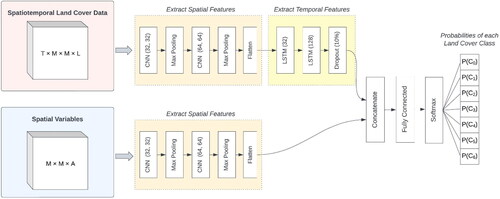
In this study, the implemented models have two input branches to leverage spatiotemporal and spatial data variables pertaining to LC change. An overview of the branched model structure is shown in Figure 5. As described in Section 2.1.3, each data sample consists of information about explanatory factors of LC change and multitemporal LC data. Thus, the spatial input branch accommodates the dimensions $M\times M\times A$ and the spatiotemporal branch accommodates the dimensions $T\times M\times M\times L$ associated with each sample. The spatial variables branch is parameterized by four convolutional layers based on previous work (van Duynhoven and Dragićević 2022b) and is implemented the same way for all model types. The layers are characterized by 32, 32, 64, and 64 filters, respectively, each with kernel dimensions of 3 × 3 (Xiao et al. 2022). The second and fourth convolutional layers are followed by 2 × 2 max pooling operations as in earlier studies (Masolele et al. 2021). The resulting feature maps are flattened and concatenated with the outputs of the spatiotemporal branch of the model. The spatiotemporal branch implementation for CNN-LSTM, CNN-GRU, and CNN-TCN models includes extraction of spatial features from each timestep with four convolutional layers and two max pooling operations, which are parameterized the same as the spatial input branch. In the CNN-LSTM model, the output of the CNN layers is provided to two LSTM layers with 32 and 128 units, respectively, based on previous studies (Guo et al. 2022). CNN-GRU is also specified with two GRU layers, with 32 and 128 units, respectively, while the CNN-TCN model has two layers with 32 and 128 filters, respectively (van Duynhoven and Dragićević 2022a). The ConvLSTM model is developed with two layers specified with 32 and 128 filters, respectively, each followed by a 2 × 2 max pooling operation. Prior to merging the outputs of the spatiotemporal input branch with that of the spatial input branch, all model types apply dropout regularization of 10%. Lastly, a fully connected neural network layer with $L$ neurons is combined with the Softmax activation function (Jagannathan and Divya 2021). This produces the probabilities of each LC class $C_k$ for the next timestep, denoted as $P(C_k).$

Figure 5. An overview of the hybrid CNN-LSTM model showing the branched structure shared across all model types. Each model branch accepts the spatiotemporal LC data with dimensions $T\times M\times M\times L$ and the explanatory spatial variables with dimensions $M\times M\times A.$

2.2.1. Model optimization with weighted categorical cross-entropy

Categorical cross-entropy (CCE) loss is often applied for multi-class applications, ensuring incorrectly projected categories are backpropagated during model training procedures (Gordon-Rodriguez et al. 2020). With each sample attributed to a LC class $C,$ the ${\mathit{Loss}}_{\mathit{CCE}}$ formula stated in prior work (Sun et al. 2022) is as follows: (1) $${\mathrm{Loss}}_{\mathrm{CCE}}\left(\widehat{y},\mathrm{ }y\right)=-\sum _{c=1}^C{\widehat{y}}_c·\log \hspace{0.17em}\left(y_c\right)$$(1) where ${\widehat{y}}_c$ and $y_c$ are the one-hot encoded LC class labels representing the category of actual and projected LC, respectively. The ${\mathrm{Loss}}_{\mathrm{CCE}}$ formula (Eq. 1(1) $${\mathrm{Loss}}_{\mathrm{CCE}}\left(\widehat{y},\mathrm{ }y\right)=-\sum _{c=1}^C{\widehat{y}}_c·\log \hspace{0.17em}\left(y_c\right)$$(1) ) applies the same treatment to all training dataset examples, such that each sample has an equal effect on model parameter adjustments. To implement a cost-sensitive learning strategy, a SW term ($w_i$) can be introduced. The derivation of $w_i$ values is explained in the next section. With $w_i$ values established to regulate the influence of each sample $i$ belonging to LC class $C,$ the ${\mathrm{Loss}}_{\mathrm{WCCE}}$ formulation becomes: (2) $${\mathrm{Loss}}_{\mathrm{WCCE}}(\widehat{y},\mathrm{ }y)=-\sum _{c=1}^C{w}_i·{\widehat{y}}_c·\log \left(y_c\right)$$(2)

Conventional $w_i$ values are calculated by schemes like IFW and ENW in other studies (Brandt and Stolle 2021; Sefrin et al. 2020). These weighting schemes provide baselines for comparing effects of weighting schemes derived from the proposed approach. The square root of IFW variation is often used to smooth values (Yan et al. 2022), which is denoted as SQRT-IFW in subsequent sections. The ENW values are calculated with the open-source Python routine made available by the authors (Cui et al. 2019).

2.3. Proposed LSM-based sample weighting approach

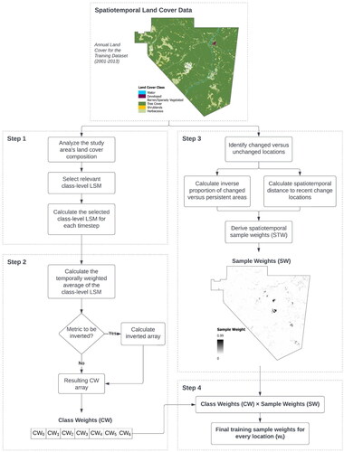
This study proposes a general framework for deriving cost-sensitive learning schemes from any class-level LSM while managing impacts of persistent samples. A flowchart depicting the methodology is shown in Figure 6 and is applied to the LC data of the Tumbler Ridge District Municipality. The four steps of the proposed LSM-based sample weighting methodology include: (1) analyzing the LC composition of the study region, (2) calculating the CW term, (3) calculating the SW term, and (4) preparing the final SWs.

Figure 6. Overview of the LSM-based sample weighting approach implementation.

Step 1: Quantifying the LC Composition of the Study Region

The LC is quantified with class-level LSMs for each timestep of the training dataset. Class-level LSMs are calculated by averaging patch-level measures for each LC type (Wu 2004). In this step, any class-level LSM can be selected based on its relevance to characteristics of the study area. For instance, if areas undergoing anthropogenic disturbances are under study, measures of shape for each LC class could be beneficial (Plexida et al. 2014; Lin et al. 2023). For each of the selected class-level metrics calculated for each data layer in the training dataset sequence, a resultant matrix of size $N\times L$ is obtained, where $N$ is the number of timesteps and $L$ is the number of LC categories plus one to accommodate background or null cell values.

Step 1 Implementation: Calculating and Interpreting Class-Level LSMs for the Tumbler Ridge District Municipality.

Given the vast forested composition and the resource-centred economy of the Tumbler Ridge District Municipality, class-level LSMs related to aggregation and shape are selected. The indicators were chosen based on previous studies identifying that patches exhibiting increasing irregular shape were associated with natural LC types, while spatial homogeneity and simpler forms conveyed human-utilized areas (Plexida et al. 2014; Lin et al. 2023). Extant work also showed the importance of patch density, contiguity, and interspersion as class-level indicators for regions dominated by forests (Griffith 2004) and mining-impacted areas (Lausch and Herzog 2002). Therefore, eight measures are used to characterize the class-level configuration of the study region, including: interspersion-juxtaposition index (IJI), patch density (PD), percentage of like adjacencies (PLADJ), largest shape index (LSI), average circumscribing circle (CIRCLEMN), standard deviation of contiguity (CONTIGSD), mean fractal dimension index (FRACMN), and standard deviation shape index (SHAPESD). All class-level LSMs are calculated with methods from the open-source landscapemetrics R package (version 1.5.5) (Hesselbarth et al. 2019). Of the hundreds of class-level LSMs described in the literature, the selection was limited to indicators found to be both relevant to the case study area and available in the open-source R package implementation. An example of the class-level LSMs obtained for the 2001 LC of the region is shown in Table 1. For each class-level metric, a matrix of size $N\times L$ is obtained, where $N=11\mathrm{ }$ (excluding the training label) and $L=7,$ corresponding with the one-hot encoding described in Section 2.1.3.

Table 1. The selected class-level LSMs calculated for the 2001 LC of Tumbler Ridge, British Columbia.

LC Class	Class area (km^2)	IJI (%)	PD (patch/ha)	PLADJ (%)	LSI	CIRCLEMN	CONTIGSD	FRACMN	SHAPESD
Water	6.11	48.23	0.35	59.72	33.18	0.52	0.22	1.05	0.75
Developed	2.02	51.57	0.01	83.89	7.61	0.54	0.29	1.07	0.99
Barren/Sparsely Vegetated	13.06	56.60	0.60	68.98	37.38	0.50	0.18	1.04	0.72
Tree Cover	1373.59	50.13	0.92	97.18	36.09	0.49	0.19	1.04	0.93
Shrublands	16.64	46.22	4.34	29.31	96.15	0.47	0.14	1.03	0.32
Herbaceous	165.93	45.88	3.78	77.64	96.22	0.53	0.22	1.06	0.77

Considering the measures of aggregation (PD, PLADJ, and LSI), each suggest homogeneity of the developed class in the observed 2001 LC data. In particular, the LSI value closer to one suggests developed areas are most aggregated. The IJI measures indicate higher percentages of differing classes interfacing with barren or sparsely vegetated LC, while herbaceous exhibits lower interspersion with dissimilar LC types. Larger CONTIGSD indices reveal higher contiguity of the developed and herbaceous LC, with each characterized by larger contiguous patch areas on average as indicated by CIRCLEMN. The FRACMN values close to one suggest more regular, squared patches comprise each LC class (Hesselbarth et al. 2019). Lastly, increasing SHAPESD indices demonstrate greater complexity of patches forming developed and tree cover areas.

Step 2: Calculating the CW Term

Once a class-level LSM is computed for every timestep of the training dataset, the resultant matrix is used to derive the CW term and can be configured according to interpretations from Step 1. Calculating the CW term includes a weighted average operation to manage classification errors that could influence LSM calculations for a singular timestep. The steps for calculating the CW using any metric is as follows:

Step 2.1: An inverse-distance temporally weighted average is obtained from the entries in the $N\times L$ matrix. For each LC class $k,$ each data layer n has an associated class-level metric value $C_k.$ To reduce the impact of $C_k$ measures of data layer earlier in the training data sequence, the squared inverse distance is applied. Therefore, the inverse-distance temporally weighted average metric value of LC class $k$ (${\mathit{AvgC}}_k$) is computed as follows: (3) $${\mathit{AvgC}}_k=\sum _{n=0}^n{C}_{k_n}\frac{1}{{(N-n)}^2}$$(3)

If the LSM-based sample weighting scheme has been indicated to be used as-is, Step 2.1 is the last step needed to obtain the CW with respect to the selected metric. This means that the final CW array becomes $CW=\mathit{AvgC}.$ However, scenarios where lower class-level LSM values should signal higher LC type importance, an inversion step is needed.

Step 2.2: If the inverse weight is set to be calculated, an inversion operation is applied to increase the importance of smaller class-level metric values based on interpretations from Step 1. The inversion step to derive the $CW$ array is as follows: (4) $$CW=\left(1-\frac{{\mathit{AvgC}}_k}{{\mathit{AvgC}}_{\max }}\right)\times \left(\frac{{\mathit{AvgC}}_{\max }}{{\mathit{AvgC}}_{\min }}\right)+{\mathit{AvgC}}_{\min }$$(4)

Despite involvement of an inversion operation option, the LSM-based sample weighting strategy fundamentally differs from traditional inverse proportion weighting schemes because the values themselves have little to no relation with class area or sample counts. Instead, the inversion strategy uses what is known about the respective class-level metrics and their meaning with respect to the study area configuration.

Step 2 Implementation: Calculating CWs for the Tumbler Ridge District Municipality

Once the class-level LSMs are calculated and interpreted, the $11\times 7$ matrices associated with each of the eight LSMs are used to derive the $CW$ values as per Step 2. $CW$ values for IJI, CONTSD, FRACMN, and SHAPESD are computed using Step 2.1 only, meaning the relative importance of each LC class is preserved based on the reported values. Meanwhile, PD, PLADJ, and LSI suggest homogeneity of the developed class (Table 1). To prioritize LC classes with this characteristic, Steps 2.1 and 2.2 are used to invert values to ensure the anthropogenic areas have high ${CW}_k$ values. Additionally, a different aspect of spatial form measured by CIRCMN is inverted to increase importance of LC classes comprised of smaller patches on average. Table 2 summarizes the eight class-level LSMs and which spatial forms they prioritize. The relative importance of $CW$ values is displayed in Figure 7, showing which LC classes are prioritized in the LSM-based sample weighting schemes compared to conventional techniques (SQRT-IFW and ENW).

Figure 7. Comparison of relative importance assigned to weight each LC class of the study region.

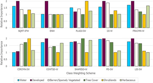
Table 2. Descriptions of the LSM-based class weighting schemes derived from selected measures of aggregation and shape.

Class-level Metric Type	Class Weighting Scheme Name	Acronym	Class Weight Derivation Strategy (i.e. direct usage or invert metric values?)	Purpose (i.e. which aspects of the configuration or composition determine LC class importance?)
Aggregation	Interspersion and Juxtaposition Index Weight	IJI-W	IJI measures computed for each class are provided as the respective CWs	Increase the importance of LC types that are more interspersed with different LC types
	Inverse Patch Density Weight	PD-IW	Inverting the patch density measures of the LC classes	Increase the importance of classes with less patch density or fewer patches, assuming more aggregated classes will exhibit less frequent change
	Inverse Percentage of Like Adjacencies Weight	PLADJ-IW	Inverting the percentage of like adjacencies measures computed for each class	Increase the weights associated with classes with mostly disaggregated patches; minimize the influence of classes with increasingly homogeneous patches
	Inverse Landscape Shape Index Weight	LSI-IW	Inverting the landscape shape indices of all LC classes	Increase the importance of compact classes, assuming aggregated classes require additional weight allocated to less frequent changes
Shape	Inverse Mean of Circumscribing Circle Weight	CIRCMN-IW	Inverting the measures describing the average circumscribing circle size for patches belonging to each class	Increase the importance of classes in which patches tend to be small; decrease the influence of classes in which patches tend to be large
	Standard Deviation of Contiguity Index Weight	CONTSD-W	The standard deviation of contiguity for each LC class	Increase the importance of classes that have greater diversity of contiguity across all patches belonging to the class
	Mean Fractal Dimension Index Weight	FRACMN-W	The mean fractal dimension index is provided directly for each CW	Increase the importance of classes characterized primarily by irregularly shaped patches; lower the importance of classes in which the average shape across patches is squared
	Standard deviation of Shape Indices Weight	SHAPESD-W	The standard deviation shape index for each LC class is provided directly for each CW	Increase the importance of classes that have greater variation of shape indices, ensuring classes with more variable patch shape complexity are prioritized

Step 3: Calculating the SW Term for Managing Changed and Persistent Areas

Once the CWs are calculated, the concurrent effects of disproportionate changed versus persistent areas must also be mitigated. An existing spatiotemporal weighting scheme (STW) (van Duynhoven and Dragićević 2022b) is used to increase the importance of LC change samples undergoing recent and nearby changes within a sample’s spatiotemporal neighbourhood. The computation is as follows:

Step 3.1: For each training data sample of dimensions $T\times M\times M,$ determine if one or more changes took place at the central cell location. If the LC of the central location is one type across all timesteps, the sample is considered persistent. Otherwise, it is marked as changed.

Step 3.2: Calculate the base weight of the persistent and changed samples according to their inverse proportion. Comparing two reference maps in the training data sequence, the number of persistent cells ($P$) and the number of transitioned samples ($D$) are used to initialize weights of persistent samples (${SW}_{p_i}$) as follows: (5) $${SW}_{p_i}=\frac{D}{(P+D)}$$(5)

Step 3.3: Lastly, changed SWs (${SW}_{c_i}$) are calculated as follows: $${SW}_{c_i}=\mathrm{ }\frac{P}{\left(P+D\right)}\times \mathrm{ }\frac{1}{d_{cl}^2}$$ (6) $$=\frac{P}{(P+D)}\times \frac{1}{{{(x-x_{cl})}^2+{(y-y_{cl})}^2+(t_n-t_{cl})}^2}$$(6) where $d_{cl}$ is the spatiotemporal distance to the most recent change location $(x_{cl},\mathrm{ }{y}_{cl},$ $t_{cl})$ in the training data sample with a power parameter of two is applied to the $d_{cl}$ term to minimize the impact of samples earlier undergoing changes.

Step 3 Implementation: Calculating SWs for the Tumbler Ridge District Municipality

First, Step 3.1 is carried out on each of the 1,752,603 samples obtained for the study region, where each sample maintains the dimensions of $12\times 9\times 9.$ In Step 3.2, the most recent years in the training dataset ($t_{2012}$ and $t_{2013}$) are used to calculate the $P$ and $D$ terms because less than 1% of the study area underwent change at any given year (Figure 3). Additionally, the finer spatial resolution and more numerous samples available for the Tumbler Ridge region introduce greater imbalance than initial applications of STW (van Duynhoven and Dragićević 2022b). Weights of persistent samples (${SW}_{p_i}$) and changed samples (${SW}_{c_i}$) are initialized, and the resulting SW map is included in Figure 6.

Step 4: Preparing the Final SWs

In the last step, CWs and SWs can be combined to manage multidimensional imbalances as in previous work (Nguyen et al. 2019). The full SW formulation combines the two intermediate weights obtained to manage the importance of changed areas (${SW}_{c_i}$ or ${SW}_{p_i}$) and the relative importance of the respective classes (${CW}_k$). Training samples which have undergone change are provided with the weight factor $w_{c_i}$ as follows: (7) $$w_{c_i}=\mathrm{ }{SW}_{c_i}\times {CW}_k\mathrm{ }$$(7)

The changed SW factor ($w_{c_i}$) ensures that transitions occurring across all classes have increased importance, with any changes to classes with greater $CW$ values allotted the highest importance. Conversely, training data samples of persistent areas are provided with the weight factor $w_{p_i}\mathrm{ }$ as follows: (8) $$w_{p_i}={SW}_{p_i}\times {CW}_k\mathrm{ }$$(8)

The persistent SW factor ($w_{p_i}$) manages the impact of persistent areas associated with larger $CW$ values through the ${SW}_{p_i}$ term. This ensures persistent areas of a highly important class k do not become excessively influential to the model’s learned parameters via the ${\mathrm{Loss}}_{\mathrm{WCCE}}$ function (Eq. 2(2) $${\mathrm{Loss}}_{\mathrm{WCCE}}(\widehat{y},\mathrm{ }y)=-\sum _{c=1}^C{w}_i·{\widehat{y}}_c·\log \left(y_c\right)$$(2) ). This has been presented at the beginning of this section, with steps outlined in Figure 6.

2.4. Experiment setup

2.4.1. DL experiment settings

Each model type is implemented with Python 3.9.1 (van Rossum 2009), TensorFlow 2.5.0 (Ghemawat et al. 2016), and the Keras API (Chollet 2015). The CNN-TCN model is implemented also with the methods available from Keras-TCN 3.4.0 (Remy 2020). The Adam gradient descent optimization procedure was used for all model types (Sun et al. 2022), with an initial learning rate set to 0.0001 (Masolele et al. 2021). The batch size specified to train each model is 128 samples. Model training also included procedures for reducing learning rates or terminating the training process when model improvements were no longer beneficial (Naushad et al. 2021), implemented by the Tensorflow callback functions called ‘ReduceLROnPlateau’ and ‘EarlyStopping.’

The experimental LSM-based SW configurations are compared against three baselines. The first is an unweighted baseline, which uses the unweighted ${\mathrm{Loss}}_{\mathrm{CCE}}$ function from Eq. (1)(1) $${\mathrm{Loss}}_{\mathrm{CCE}}\left(\widehat{y},\mathrm{ }y\right)=-\sum _{c=1}^C{\widehat{y}}_c·\log \hspace{0.17em}\left(y_c\right)$$(1) . The IFW and ENW schemes (Brandt and Stolle 2021; Sefrin et al. 2020) are also used to train baselines to compare effects on model performance. Knowing that the imbalance of changed versus persistent cells is highly influential to model outcomes, CWs derived from SQRT-IFW and ENW are combined with the SW terms derived in Step 3 to facilitate an equal comparison with the outcomes of the proposed approach.

The proposed LSM-based SW schemes are parameterized with eight different class-level LSMs to demonstrate the utility of the framework and the effects of SWs derived from spatial structure. Four LSM-based SW schemes are formulated directly using LSM values from IJI, FRACMN, CONTSD and SHAPESD. These are labelled with the postfix-W (IJI-W, FRACMN-W, CONTSD-W and SHAPESD-W) as shown in Table 2. Four configurations of the LSM-based SW technique are explored using the inversion scheme (Table 2), indicated with the postfix-IW (PD-IW, PLADJ-IW, LSI-IW and CIRCMN-IW). The SW term calculated in Step 3 is incorporated in all but the unweighted baseline configuration.

2.4.2. Model assessment

An assessment of the outputted locations and quantities of changes overall and for each LC class is conducted for each model type. Overall accuracy measures are unreliable to evaluate model performance in the presence of imbalanced LC data because of the larger number of samples belonging to majority categories (Nikparvar and Thill 2021). Hence, the primary assessment approach involves metrics focussed on forecasting LC change. Such metrics are referred to as three-map comparison measures (Ahmed et al. 2013). The principal measure used in this study is figure of merit (FOM), which conveys the correspondence of observed and modelled changes with values from 0% (i.e., no agreement) to 100% (i.e., perfect agreement) (Pontius et al. 2008). Two other measures computed from terms comprising FOM include producer’s accuracy (PA) and user’s accuracy (UA) (Pontius et al. 2008). PA and UA differ from FOM by instead providing the ratio of correctly changed areas versus all projected changes or all observed changes, respectively. It should also be noted that PA and UA are synonymous with measures of Recall and Precision, which are also common measures used to compare remote sensing images (Foody 2020). In addition to FOM, PA, and UA, previous studies recommend that their constituent terms be stated to further distill land change model outcomes (Varga et al. 2020). This includes reporting the number of correctly simulated changes (hits), the number of persistent changes incorrectly simulated as changed (false alarms), the number of changed areas simulated incorrectly as persistent (misses), and the number of changes allocated to an incorrect gaining class (wrong hits) (Ahmadlou et al. 2022).

Next, the per-class changes forecasted and observed for each LC category are compared. While it would seem appropriate to use the previous class-level LSMs for this task (Amiri et al. 2017), neither ${\mathrm{Loss}}_{\mathrm{CCE}}$ or ${\mathrm{Loss}}_{\mathrm{WCCE}}$ explicitly optimize spatial pattern agreement in this study. Instead, the total changed areas forecasted or observed can convey whether realistic amounts of land changes were simulated (Aguejdad et al. 2017). For each LC class, the projected change (PC) measure provides the summation of hits and false alarms, while observed change (OC) conveys the sum of hits and misses. Assessing incongruence of PC versus OC was used instead of comparing exact locational agreements because of the small number (or absence) of transitions attributable to some LC types in the imbalanced dataset of 1.7 million cells. This motivates further evaluation of how much the forecasted allocations of each LC type deviate from their real-world locations via the error in allocation (EIA) measure (Paegelow et al. 2014). EIA is obtained by computing the average Euclidean distance of the respective error locations to the nearest real-world patch belonging to the same category (Paegelow et al. 2014). The resulting EIA values indicate the severity of allocation errors, where lower averaged allocation error distances suggest better forecasts of LC changes. Conversely, higher EIA values suggest a model projected a LC class further away from its real-world location.

The assessment was conducted with Python 3.9.1, using functionalities from Numpy 1.21.5, GDAL 3.3.0, and RasterStats 0.17.0. The FOM values obtained with respect to LC forecasted for 2015 are summarized across all model types to identify any consistency across experimental configurations. The top three LSM-based sample weighting schemes are chosen based on this initial assessment for the subsequent analysis steps described. Of the selected configurations, results of models yielding the highest FOM values for 2019 are displayed with elements comprising FOM to visually assess error locations (Ahmed et al. 2013).

3. Results

3.1. Overall effects of class weighting schemes on one-year LC change forecasts

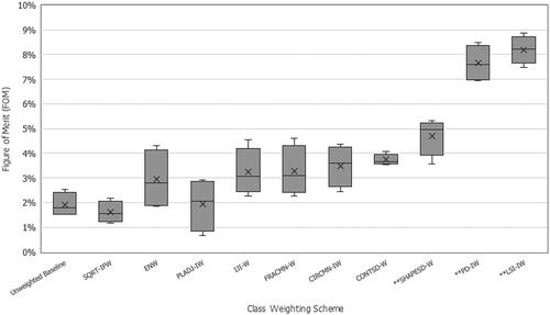
Overall, the LSM-based sample weighting schemes produced models with FOM measures consistent to or better than the baseline configurations for the 2015 LC forecasts. The effects were observed across the four model types and are presented in Figure 8. SHAPESD-W, PD-IW, and LSI-IW schemes generated typically higher FOM measures than the baselines. All models trained with the PD-IW and LSI-IW schemes had the highest FOM measures (Figure 8). Additionally, most of the FOM values obtained with SHAPESD-W exceeded the upper quartiles for all but PD-IW and LSI-IW.

Figure 8. Boxplot of FOM measures obtained by comparing the real-world and simulated changes for 2015 across all model types. The three class weighting schemes attributed to the highest average FOM values are shown with the prefix (**).

3.2. Forecasted LC change from 2015 to 2019

Taking the top three LSM-based SW results from the previous assessment (Figure 8), outcomes of the five-year projection are compared with the baseline configurations. As seen in Figure 9a, the highest FOM values after the five-year projection were approximately 15.2, 13.4, 12.4, and 11.1%, obtained by CNN-LSTM_PD-IW, ConvLSTM_PD-IW, CNN-TCN_PD-IW, and CNN-GRU_PD-IW, respectively. With respect to PA (Figure 9b), the proportion of the study area forecasted correctly as changed versus all observed changes remains the highest with the PD-IW scheme for all model types. All PA values exhibit a downward trend after the 2016 LC projections, highlighting a decline in the quantity of correct changes forecasted as the number of observed changes accumulates. Meanwhile, as presented in Figure 9c, the UA demonstrates the proportion of area forecasted correctly as changed versus all projected changes is highest for CNN-GRU_Unweighted, CNN-LSTM_LSI-IW, CNN-TCN_SHAPESD-W, and ConvLSTM_SHAPESD-W configurations for most timesteps in the five-year span. The low FOM metric obtained with CNN-GRU_Unweighted stems from the small number of projected changes being allocated to correct locations (Figure 10a). CNN-LSTM_LSI-IW attained notable FOM and UA values, indicating a higher quantity of projected changes were at the correct locations. Overall, PD-IW and LSI-IW showed consistently better results across all models in FOM and PA measures.

Figure 9. The FOM, PA, and UA calculated with respect to the cumulative LC changes correctly projected from 2015 to 2019.

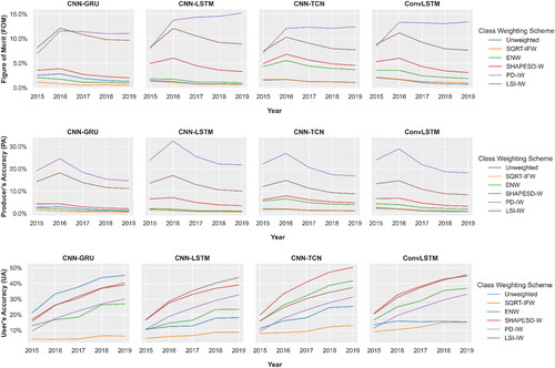
Figure 10. Trends of FOM components attributed to each class weighting scheme for the 2019 land cover forecasts. The box plots depict the percent of study area extent identified as (a) correctly forecasted changes, (b) false alarms, (c) missed changes, and (d) changes forecasted as the incorrect class summarized across all model types.

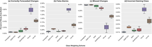
Next, the trends in FOM components for the baseline and LSM-based SW outcomes are compared across all model types for the 2019 LC forecast, with values presented in Figure 10. With respect to the FOM components, PD-IW allocates the largest quantity of changes to the correct locations, regardless of model type (Figure 10a). All model types trained with the PD-IW scheme projected the largest number of correct changes, accounting for 0.65–0.97% of the study area extent. PD-IW also facilitated fewer errors stemming from missed changes (Figure 10c). However, these outcomes exhibited the highest quantity of false alarms (Figure 10b) and assigned more changed areas as incorrect gaining categories (Figure 10d). LSI-IW enabled moderate performance gains versus the baseline configurations, showing fewer false alarms and incorrectly gaining classes assigned to observed transitioned areas. SHAPESD-W aided small increases in quantity of correctly forecasted changes across the model types compared to the baselines, with fewer areas identified as false alarms and missed changes than SQRT-IFW.

3.3. Evaluating per-class changes for 2019

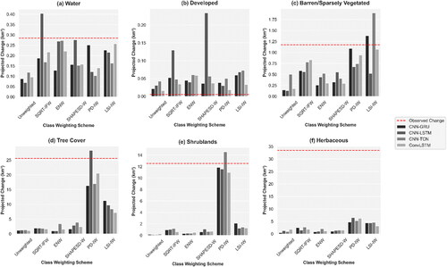
After assessing the LC change allocations, outcomes of models trained with the three baselines and selected LSM-based SWs are compared to assess per-class LC changes projected for 2019. By comparing the cumulation of observed versus projected changes, rarer classes (i.e., developed) clearly undergo the smallest amount of real-world change between 2015 and 2019 (Figure 11b). Meanwhile, increased area classified as water was not over-projected by any LSM-based sample weighting scheme despite its comparatively small area. Similarly, the PD-IW and LSI-IW schemes facilitated more realistic quantities of transitioned areas attributed to the barren or sparely vegetated LC class across the respective model types. The classes associated with the most transitioned areas over the five-year period include tree cover, shrublands, and herbaceous LC (Figure 11d–f). PD-IW enabled all model types to forecast more realistic quantities of change to areas designated as tree cover and shrublands, and higher amounts of change for the herbaceous class than other configurations.

Figure 11. Comparison of cumulative projected and observed changes from 2015 to 2019 for each LC class and the selected class weighting schemes.

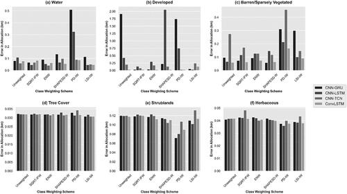
Next, the EIA assessment shows the severity of changes allocated to the wrong locations. All model types and CW scheme combinations showed an average distance of errors projected 30–40 m from real-world locations for tree cover and herbaceous LC types (Figure 12d and f). In other words, the changes allocated to these categories were on average misallocated by a distance equivalent to the size of one cell. Models trained with PD-IW showed reduced distances between the error and the real-world locations by 20–40 m for the shrublands class (Figure 12e). While CNN-TCN_PD-IW and ConvLSTM_PD-IW showed low EIA for water and developed LC classes, changed areas for these classes allocated by CNN-GRU_PD-IW, CNN-LSTM_PD-IW and CNN-LSTM_SHAPESD-W were distinctly further from real-world locations (Figure 12a–c).

Figure 12. Comparison of the average error in allocation distances computed with respect to the real-world 2019 LC for each class and the selected class weighting schemes.

3.4. Visual assessment of 2019 LC forecasts

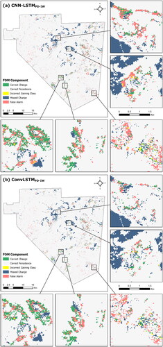
The CNN-LSTM_PD-IW and ConvLSTM_PD-IW models were selected for visual comparison as they showed the highest overall FOM value and a high FOM with lower errors, respectively. The false alarms scattered across the study region are visibly less with ConvLSTM_PD-IW compared to CNN-LSTM_PD-IW (Figure 13). Overall, ConvLSTM_PD-IW produced fewer ‘salt-and-pepper’ errors (Figure 13b). In the outputs produced by CNN-LSTM_PD-IW and ConvLSTM_PD-IW, false alarms are often adjacent to correctly changed areas. The areas indicated as missed changes are mostly related to expansions of herbaceous LC, which corresponds with the low quantities of forecasted changes for this class (Figure 11f). Areas indicated as missed changes appear in similar locations across the two maps of projected LC.

Figure 13. Mapped FOM components of the 2019 LC change forecasts shown for (a) CNN-LSTM_PD-IW and (b) ConvLSTM_PD-IW displayed using the NAD 1983 UTM 10N projected coordinate system.

4. Discussion

Overall, the results of the case study showed that implementations of the proposed LSM-based sample weighting scheme were advantageous to all model types explored. By deriving CWs from measures of relative spatial complexity, the varying conditions of each LC type can be encoded to influence model training. The LSM-based framework provides an alternative to proportion-based weighting schemes specialized for categorical geographic datasets. While it is acknowledged there are a vast number of class-level LSM types to choose from (i.e., Hesselbarth et al. 2019), the demonstration of the proposed procedure leveraged indicators of the respective aggregation or shape of each LC class. Regardless of model architecture, LSM-based SWs underpinned by measures of patch density (PD-IW), shape irregularity (LSI-IW) and shape variation (SHAPESD-W) produced consistent and notable improvements to overall measures of LC change (Figures 8 and 9). Because spatial homogeneity and simpler structures were previously attributed to human-utilized areas (Plexida et al. 2014; Lin et al. 2023), PD-IW and LSI-IW schemes implement higher importance to less fragmented and more compact LC types. Meanwhile, the SHAPESD-W scheme prioritized a different perspective of the landscape structure, instead boosting the significance of LC types exhibiting more variability in patch shapes. FOM values attained by PD-IW and LSI-IW were strikingly higher than all other experimental configurations (Figure 9). The FOM values ranged from 10 to 15% for the different model architectures, which is similar to values obtained for other 5-year projections (Lin et al. 2023) and exceeding models generating 5- and 6-year projections (Varga et al. 2020; van Duynhoven and Dragićević 2022b).

Although the two weighted baselines (SQRT-IFW and ENW) allotted highest relative importance to examples of developed areas as seen with PD-IW and LSI-IW (Figure 6), the conventional approaches dismiss the LC types important to the area. This is a known problem of frequency-weighting approaches, which can be detrimental to important samples associated with majority classes (Nguyen et al. 2019). Instead, PD-IW and LSI-IW were selected and specified based on activities and influences affecting the landscape, consequently assigning per-class importance that better aligned with the characteristics of the region (Figure 6). This led to distinctive improvements in overall assessments and per-class projections for these LC types (Figures 8–12). Studies investigating forest-dominated study areas found patch density to be an important indicator of landscape influences (Griffith 2004), the same indicator underpinning the PD-IW scheme.

While CNN-LSTM_PD-IW obtained the highest FOM values, ConvLSTM_PD-IW projected fewer errors overall (Figure 9), more realistic quantities of change (Figure 11), and less severe errors for each LC class (Figure 12). This motivated the visual comparison, where it was apparent that the higher FOM values achieved by CNN-LSTM_PD-IW were accompanied by more errors. This outcome is similar to previous LC modelling studies showing increased FOM and decreased false alarms attributed to the ConvLSTM architecture (van Duynhoven and Dragićević 2022b). From the visual assessment, it is apparent that the numerous ‘salt-and-pepper’ errors seen in the previous work (van Duynhoven and Dragićević 2022b) are less widespread in this research (Figure 13). Instead, errors appear more contiguous, suggesting that the newly proposed framework helps to minimize modelling of unrealistic change events. However, the per-class and visual assessments show a need for further improvement. For instance, no experimental configuration forecasted realistic expansion of the herbaceous LC class (Figure 11). The homogeneous appearance of the expanding herbaceous LC suggests anthropogenic activity. Therefore, ensemble modelling (i.e., Ahmadlou et al. 2022) or integration with models capable of projected emergent and stochastic behaviours (i.e., Xing et al. 2020) may complement the data-driven modelling approaches used in this research work.

4.1. Limitations and future directions

Though FOM values obtained in the experiments are considered reasonable given the small amounts of LC change (Pontius et al. 2008), the overlap between real and projected changes can still be improved. The experiment outcomes indicated that not all LSMs resulted in beneficial SWs for the study area. However, it should be noted that conclusions about the generalizability of the specific set of class-level LSMs used to derive the CW terms cannot be stated without more rigorous assessments on other study areas exhibiting different landscape compositions. This is expected because CWs derived from class-level LSMs are not exempt from the enduring debates about which measures are ideal for certain landscape structures and processes. Consequently, it is necessary to investigate the effects of class-level LSMs inserted in the sample weighting framework for different study area compositions and model implementations. Additionally, the effects of LC classification accuracy and spatial resolution should also be examined due to their reported impacts on LSMs (Amiri et al. 2017) and DL models (van Duynhoven and Dragićević 2019). Given that shrubland, herbaceous, and barren LC types have notably overlapping qualities (Section 2.1.1), identifying and managing misclassifications via SWs may also be beneficial. Furthermore, class-level LSMs were previously demonstrated to exhibit large variations when spatial resolution and study area extents were adjusted (Wu 2004). While this does impact the transferability of the specific class-level LSMs found to produce the most ideal SWs in the presented case study, this does not impact the generalizability of the proposed sample weighting approach because it accepts any class-level LSM. Lastly, it is recommended that an assessment of landscape configuration agreement is added in future evaluations to complement measures of quantity and allocation as demonstrated in previous studies (Pickard et al. 2017) following adjustments to the objective function.

5. Conclusions

The goal of this study was to propose a cost-sensitive learning strategy which incorporated measures of spatial structure for LC classes. This was done by defining a specialized geospatial sample weighting scheme derived from class-level LSMs, producing varying SWs for LC classes based on their respective spatial configurations. It is known that spatial metrics used to analyze LC types provide meaningful indications of relative landscape form and composition. However, there is an absence of literature exploiting LSMs to prioritize certain LC classes in data-driven models. Furthermore, there is a lack of spatialized cost-sensitive learning strategies, which led prior works to use aspatial sample weighting schemes such as conventional proportion-based weighting techniques. Instead, this work presents a framework to generate varying penalties based on a selection of class-level LSMs and knowledge of notable spatial patterns characterizing a study area. This supports integration of knowledge about an area’s significant spatial arrangements and avoids the tedious procedure of manually specifying SWs. With new spatialized cost-sensitive learning strategies, ML and DL methods can become a viable choice for leveraging large amounts of geospatial data in future land change studies.

Since the proposed methodology is agnostic to any class-level LSM, a case study of forecasting LC changes with DL models in a severely imbalanced study area demonstrated how relevant indicators can be inserted in the presented sample weighting strategy. To illustrate the procedure, eight LSMs were selected to parameterize different experimental configurations. In this example, the computed SWs prioritized different LC types based on their overall aggregation or shape. The results showed several of the LSM-based SWs prompted notable improvements in LC change forecasted compared to unweighted and traditional sample weighting schemes (SQRT-IFW and ENW). This was reflected by distinctive increases of the FOM measure and its constituent terms. The performance improvements were maintained throughout the multi-year LC projections across the different spatiotemporal DL model architectures.

In conclusion, this study shows how exploiting class-level measures of landscape structure can help models to successfully project more realistic changes across more LC categories. Future studies can leverage the agnostic framework to derive SWs with class-level LSMs relevant to new study areas and spatial configurations. While the proposed approach was employed for multitemporal data, class-level LSMs can also be obtained for static spatial datasets by discarding the temporal weighted averaging step. This study contributes to the advancement of specialized geospatial cost-sensitive learning strategies to improve ML and DL methodologies for any application using categorical geographic data, including modelling forest changes, forest disturbances, wetland and habitat fragmentation, or urban expansion.

Acknowledgments

The authors are grateful for the constructive feedback and suggestions provided by the four anonymous reviewers and the journal Editor. The authors acknowledge and thank the Natural Sciences and Engineering Research Council (NSERC) of Canada for fully supporting this study through the Postgraduate Scholarship-Doctoral Grant (PGS-D) and the Discovery Grant (RGPIN-2017-03939) awarded to the first and second authors, respectively. The authors are also appreciative of the support provided by the Simon Fraser University Library Open Access Fund. Lastly, the authors would like to thank the personnel from the Digital Research Alliance of Canada for the technical assistance and for enabling the experiments to be run for this study via the Advanced Research Computing platform.

Disclosure statement

No potential conflict of interest was reported by the authors.

Data availability statement

The open datasets used this study include the Global Land Cover Mapping and Estimation (GLanCE) annual 30 m (m) Version 1 data product https://lpdaac.usgs.gov/products/glance30v001/ (accessed 3 January 2023), the Terra Advanced Spaceborne Thermal Emission and Reflection Radiometer (ASTER) Global Digital Elevation Model (GDEM) Version 3 (ASTGTM) https://lpdaac.usgs.gov/products/astgtmv003/ (accessed 2 December 2022), Population Centers and Digital Boundary Files of Canadian Provinces and Territories https://www12.statcan.gc.ca/census-recensement/2011/geo/bound-limit/bound-limit-2016-eng.cfm (accessed 2 December 2022), Canadian Census Road Network https://open.canada.ca/data/en/dataset/57d5ffae-3048-4a19-9b4c-eab12f6322c5 (accessed 2 December 2022), British Columbia Railway Network https://catalogue.data.gov.bc.ca/dataset/railway-track-line (accessed 3 December 2022), Lakes https://catalogue.data.gov.bc.ca/dataset/freshwater-atlas-lakes (accessed 3 December 2022), Rivers https://catalogue.data.gov.bc.ca/dataset/freshwater-atlas-rivers (accessed 2 December 2022), Parks and Protected Areas https://catalogue.data.gov.bc.ca/dataset/parks-and-protected-areas-regional-boundaries (accessed 2 December 2022), Agricultural Land Reserve https://catalogue.data.gov.bc.ca/dataset/alc-alr-polygons (accessed 2 December 2022), and Canadian Cartographic Boundary File https://open.canada.ca/data/en/dataset/a883eb14-0c0e-45c4-b8c4-b54c4a819edb (accessed 28 February 2023).

Additional information

Funding

This research was funded by the Natural Sciences and Engineering Research Council (NSERC) of Canada.

References

- Abrams M, Tsu H, Hulley G, Iwao K, Pieri D, Cudahy T, Kargel J. 2015. The advanced spaceborne thermal emission and reflection radiometer (ASTER) after fifteen years: review of global products. Int J Appl Earth Observ Geoinf. 38:292–301. doi: 10.1016/j.jag.2015.01.013.
- Aguejdad R, Houet T, Hubert-Moy L. 2017. Spatial validation of land use change models using multiple assessment techniques: a case study of transition potential models. Environ Model Assess. 22(6):591–606. doi: 10.1007/s10666-017-9564-4.
- Ahmadlou M, Karimi M, Pontius RG. 2022. A new framework to deal with the class imbalance problem in urban gain modeling based on clustering and ensemble models. Geocarto Int. 37(19):5669–5692. doi: 10.1080/10106049.2021.1923826.
- Ahmed B, Ahmed R, Zhu X. 2013. Evaluation of model validation techniques in land cover dynamics. IJGI. 2(3):577–597. doi: 10.3390/ijgi2030577.
- Amiri BJ, Asgarian A, Sakieh Y. 2017. Introducing landscape accuracy metric for spatial performance evaluation of land use/land cover change models. Geocarto Int. 32(11):1171–1187. doi: 10.1080/10106049.2016.1206628.
- Arevalo P, Stanimirova R, Bullock E, Zhang Y, Tarrio K, Turlej K, Hu K, et al. 2022. Global land cover mapping and estimation yearly 30 m V001. Distributed by NASA EOSDIS Land Processes DAAC. 2022. doi: 10.5067/MEaSUREs/GLanCE/GLanCE30.001.
- Asempah M, Sahwan W, Schütt B. 2021. Assessment of land cover dynamics and drivers of urban expansion using geospatial and logistic regression approach in WA Municipality, Ghana. Land. 10(11):1251. doi: 10.3390/land10111251.
- Brandt J, Stolle F. 2021. A global method to identify trees outside of closed-canopy forests with medium-resolution satellite imagery. Int J Remote Sens. 42(5):1713–1737. doi: 10.1080/01431161.2020.1841324.
- Broeck WAVd, Goedemé T, Loopmans M. 2022. Multiclass land cover mapping from historical orthophotos using domain adaptation and spatio-temporal transfer learning. Remote Sens. 14(23):5911. doi: 10.3390/rs14235911.
- Cao C, Dragićević S, Li S. 2019. Short-term forecasting of land use change using recurrent neural network models. Sustainability (Switzerland). 11(19):5376. doi: 10.3390/su11195376.
- Cho K, van Merrienboer B, Gulcehre C, Bahdanau D, Bougares F, Schwenk H, Bengio Y. 2014. Learning phrase representations using RNN encoder–decoder for statistical machine translation. In Proceedings of the 2014 Conference on Empirical Methods in Natural Language Processing (EMNLP), 1724–34. Stroudsburg, PA, USA: Association for Computational Linguistics. doi: 10.3115/v1/D14-1179.
- Chollet F. 2015. Keras: the Python Deep Learning Library. Keras.Io. Astrophysics source code library. 2015. https://keras.io/.
- Cui Y, Jia M, Lin TY, Song Y, Belongie S. 2019. Class-balanced loss based on effective number of samples. In. Proceedings of the IEEE Computer Society Conference on Computer Vision and Pattern Recognition, 2019-June, 9260–9269. doi: 10.1109/CVPR.2019.00949.
- Esri. 2023. Train Deep Learning Model (Image Analyst). ArcGIS Pro 3.1 Tool Reference. 2023. https://pro.arcgis.com/en/pro-app/latest/tool-reference/image-analyst/train-deep-learning-model.htm.
- Foody GM. 2020. Explaining the unsuitability of the Kappa Coefficient in the assessment and comparison of the accuracy of thematic maps obtained by image classification. Remote Sens Environ. 239(March):111630. doi: 10.1016/j.rse.2019.111630.
- Fotheringham AS, Rogerson PA. 1993. GIS and spatial analytical problems. Int J Geogr Inf Syst. 7(1):3–19. doi: 10.1080/02693799308901936.
- Frazier AE, Kedron P. 2017. Landscape metrics: past progress and future directions. Curr Landsc Ecol Rep. 2(3):63–72. doi: 10.1007/s40823-017-0026-0.
- Friedl MA, Woodcock CE, Olofsson P, Zhu Z, Loveland T, Stanimirova R, Arevalo P, Bullock E, Hu K-T, Zhang Y, et al. 2022. Medium spatial resolution mapping of global land cover and land cover change across multiple decades from landsat. Front Remote Sens. 3:0–15. doi: 10.3389/frsen.2022.894571.
- Ghemawat S, Zheng X, Moore S, Abadi M, Dean J, Chen Z, Kudlur M, et al. 2016. TensorFlow: a system for large-scale machine learning. In Proceedings of the 12th USENIX Symposium on Operating Systems Design and Implementation, OSDI 2016, p. 265–83.
- Gordon-Rodriguez E, Loaiza-Ganem G, Pleiss G, Cunningham JP. 2020. Uses and abuses of the cross-entropy loss: case studies in modern deep learning. In Proceedings on “I Can’t Believe It’s Not Better!” at NeurIPS Workshops, PMLR 137, p. 1–10.
- Griffith JA. 2004. The role of landscape pattern analysis in understanding concepts of land cover change. J Geogr Sci. 14(S1):3–17. doi: 10.1007/BF02873085.
- Guo Y, Zhang S, Yang J, Yu G, Wang Y. 2022. Dual memory scale network for multi-step time series forecasting in thermal environment of aquaculture facility: a case study of recirculating aquaculture water temperature. Expert Syst Appl. 208(May 2021):118218. doi: 10.1016/j.eswa.2022.118218.
- Halseth G, Markey S, Ryser L, Hanlon N, Skinner M. 2017. Exploring new development pathways in a remote mining town: the case of Tumbler Ridge, BC Canada. J Rural Community Dev. 12(2–3):1–22.
- Harati S, Perez L, Molowny-Horas R. 2020. Integrating neighborhood effect and supervised machine learning techniques to model and simulate forest insect outbreaks in British Columbia, Canada. Forests. 11(11):1215. doi: 10.3390/f11111215.
- He H, Garcia EA. 2009. Learning from imbalanced data. IEEE Trans Knowl Data Eng 21(9): 1263–1284. doi: 10.1109/TKDE.2008.239.
- Hesselbarth MH, Sciaini M, With KA, Wiegand K, Nowosad J. 2019. Landscapemetrics: an open-source r tool to calculate landscape metrics. Ecography. 42(10):1648–1657. doi: 10.1111/ecog.04617.
- Hewage P, Behera A, Trovati M, Pereira E, Ghahremani M, Palmieri F, Liu Y. 2020. Temporal convolutional neural (TCN) network for an effective weather forecasting using time-series data from the local weather station. Soft Comput. 24(21):16453–16482. doi: 10.1007/s00500-020-04954-0.
- Hochreiter S, Schmidhuber J. 1997. Long short-term memory. Neural Comput. 9(8):1735–1780. doi: 10.1162/neco.1997.9.8.1735.
- Jagannathan J, Divya C. 2021. Deep learning for the prediction and classification of land use and land cover changes using deep convolutional neural network. Ecol Inform 65:101412. doi: 10.1016/j.ecoinf.2021.101412.
- Johnson JM, Khoshgoftaar TM. 2019. Survey on deep learning with class imbalance. J Big Data. 6:27. doi: 10.1186/s40537-019-0192-5.
- Kang M, Liu Y, Wang M, Li L, Weng M. 2022. A random forest classifier with cost-sensitive learning to extract urban landmarks from an imbalanced dataset. Int J Geogr Inf Sci. 36(3):496–513. doi: 10.1080/13658816.2021.1977814.
- Karpatne A, Jiang Z, Vatsavai RR, Shekhar S, Kumar V. 2016. Monitoring land-cover changes: a machine-learning perspective. IEEE Geosci Remote Sens Mag. 4(2):8–21. doi: 10.1109/MGRS.2016.2528038.
- Kellenberger B, Marcos D, Tuia D. 2018. Detecting mammals in UAV images: best practices to address a substantially imbalanced dataset with deep learning. Remote Sens Environ. 216:139–153. doi: 10.1016/j.rse.2018.06.028.
- Lausch A, Herzog F. 2002. Applicability of landscape metrics for the monitoring of landscape change: issues of scale, resolution and interpretability. Ecol Indic. 2(1–2):3–15. doi: 10.1016/S1470-160X(02)00053-5.
- Lea C, Flynn MD, Vidal R, Reiter A, Hager GD. 2017. Temporal convolutional networks for action segmentation and detection. In Proceedings - 30th IEEE Conference on Computer Vision and Pattern Recognition, CVPR 2017, p. 1003–1012. Institute of Electrical and Electronics Engineers Inc. doi: 10.1109/CVPR.2017.113.
- LeCun Y, Bengio Y, Hinton G. 2015. Deep learning. Nature. 521(7553):436–444. doi: 10.1038/nature14539.
- Li X, Yeh AG-O. 2002. Neural-network-based cellular automata for simulating multiple land use changes using GIS. Int J Geogr Inf Sci. 16(4):323–343. doi: 10.1080/13658810210137004.
- Lin J, Li X, Wen Y, He P. 2023. Modeling urban land-use changes using a landscape-driven patch-based cellular automaton (LP-CA). Cities. 132:103906. doi: 10.1016/j.cities.2022.103906.
- Lu J, Ren K, Li X, Zhao Y, Xu Z, Ren X. 2022. From reanalysis to satellite observations: gap-filling with imbalanced learning. GeoInformatica. 26(2):397–428. doi: 10.1007/s10707-020-00426-7.
- Machemer P, Simmons C, Walker R. 2006. Refining landscape change models through outlier analysis in the Muskegon watershed of Michigan. Landsc Res. 31(3):277–294. doi: 10.1080/01426390600783426.
- Martínez S, Mollicone D. 2012. From land cover to land use: a methodology to assess land use from remote sensing data. Remote Sens. 4(4):1024–1045. doi: 10.3390/rs4041024.
- Masolele RN, De Sy V, Herold M, Marcos D, Verbesselt J, Gieseke F, Mullissa AG, Martius C. 2021. Spatial and temporal deep learning methods for deriving land-use following deforestation: a pan-tropical case study using Landsat time series. Remote Sens Environ. 264:112600. doi: 10.1016/j.rse.2021.112600.
- Mungai LM, Messina JP, Zulu LC, Qi J, Snapp S. 2022. Modeling spatiotemporal patterns of land use/land cover change in central Malawi using a neural network model. Remote Sens. 14(14):3477. doi: 10.3390/rs14143477.
- Naushad R, Kaur T, Ghaderpour E. 2021. Deep transfer learning for land use and land cover classification: a comparative study. Sensors. 21(23):8083. doi: 10.3390/s21238083.
- Nguyen HM, Demir B, Dalponte M. 2019. A weighted SVM-based approach to tree species classification at individual tree crown level using LiDAR data. Remote Sens. 11(24):2948. doi: 10.3390/rs11242948.
- Nikparvar B, Thill J-C. 2021. Machine learning of spatial data. IJGI. 10(9):600. doi: 10.3390/ijgi10090600.
- Paegelow M, Camacho Olmedo MT, Mas J, Houet T. 2014. Benchmarking of LUCC modelling tools by various validation techniques and error analysis. Cybergeo: Eur J of Geogr. doi: 10.4000/cybergeo.26610.
- Parker DC, Manson SM, Janssen MA, Hoffmann MJ, Deadman P. 2003. Multi-agent systems for the simulation of land-use and land-cover change: a review. Ann Assoc Am Geogr. 93(2):314–337. doi: 10.1111/1467-8306.9302004.
- Pedregosa F, Varoquaux G, Gramfort MBA, Michel V, Thirion B, Grisel O. 2011. Scikit-learn: machine learning in Python. J Mach Learn Res. 12:2825–2830. doi: 10.5555/1953048.2078195.
- Pickard B, Gray J, Meentemeyer R. 2017. Comparing quantity, allocation and configuration accuracy of multiple land change models. Land. 6(3):52. doi: 10.3390/land6030052.
- Plexida SG, Sfougaris AI, Ispikoudis IP, Papanastasis VP. 2014. Selecting landscape metrics as indicators of spatial heterogeneity-acomparison among Greek landscapes. Int J Appl Earth Observ Geoinf. 26(1):26–35. doi: 10.1016/j.jag.2013.05.001.
- Pontius RG, Boersma W, Castella J-C, Clarke K, de Nijs T, Dietzel C, Duan Z, Fotsing E, Goldstein N, Kok K, et al. 2008. Comparing the input, output, and validation maps for several models of land change. Ann Reg Sci. 42(1):11–37. doi: 10.1007/s00168-007-0138-2.
- Remy P. 2020. Temporal convolutional networks for Keras. GitHub Repository. 2020. https://github.com/philipperemy/keras-tcn.
- Ren Y, Lü Y, Comber A, Fu B, Harris P, Wu L. 2019. Spatially explicit simulation of land use/land cover changes: current coverage and future prospects. Earth-Sci Rev. 190:398–415. doi: 10.1016/j.earscirev.2019.01.001.
- Rossum G. V. 2009. Python language reference. Amsterdam, Netherlands: Python Software Foundation. doi: 10.1201/9781584889304.axd.
- Ryser L, Halseth G, Markey S, Gunton C, Argent N. 2019. Path dependency or investing in place: understanding the changing conditions for rural resource regions. Extr Ind Soc. 6(1):29–40. doi: 10.1016/j.exis.2018.10.009.
- Sefrin O, Riese FM, Keller S. 2020. Deep learning for land cover change detection. Remote Sens. 13(1):78. doi: 10.3390/rs13010078.
- Shi X, Chen Z, Wang H, Yeung D-Y, Wong W-K, Woo W-C. 2015. Convolutional LSTM Network: a machine learning approach for precipitation nowcasting. In Advances in Neural Information Processing Systems 28 (NIPS 2015), p. 802–810. doi: 10.1074/jbc.M200827200.
- Statistics Canada. 2023. Census Profile. 2021 Census of Population. Statistics Canada Catalogue No. 98-316-X2021001. https://www12.statcan.gc.ca/census-recensement/2021/dp-pd/prof/index.cfm?Lang=E.
- Sun P, Lu Y, Zhai J. 2022. Mapping land cover using a developed U-net model with weighted cross entropy. Geocarto Int. 37(25):9355–9368. doi: 10.1080/10106049.2021.2017017.
- Tarawneh AS, Hassanat AB, Altarawneh GA, Almuhaimeed A. 2022. Stop oversampling for class imbalance learning: a review. IEEE Access. 10:47643–47660. doi: 10.1109/ACCESS.2022.3169512.
- Turner BL, Lambin EF, Reenberg A. 2007. The emergence of land change science for global environmental change and sustainability. Proc Natl Acad Sci USA. 104(52):20666–20671. doi: 10.1073/pnas.0704119104.
- van Duynhoven A, Dragićević S. 2019. Analyzing the effects of temporal resolution and classification confidence for modeling land cover change with long short-term memory networks. Remote Sens. 11(23):2784. doi: 10.3390/rs11232784.
- van Duynhoven A, Dragićević S. 2022a. Assessing the impact of neighborhood size on temporal convolutional networks for modeling land cover change. Remote Sens. 14(19):4957. doi: 10.3390/rs14194957.
- van Duynhoven A, Dragićević S. 2022b. Mitigating imbalance of land cover change data for deep learning models with temporal and spatiotemporal sample weighting schemes. IJGI. 11(12):587. doi: 10.3390/ijgi11120587.
- Varga OG, Pontius RG, Jr, Szabó Z, Szabó S. 2020. Effects of category aggregation on land change simulation based on Corine land cover data. Remote Sens. 12(8):1314. doi: 10.3390/rs12081314.
- Wang J, Bretz M, Ali Akber Dewan M, Delavar MA. 2022. Machine learning in modelling land-use and land cover-change (LULCC): current status, challenges and prospects. Sci Total Environ. 822:153559. doi: 10.1016/j.scitotenv.2022.153559.
- Wang H, Zhao X, Zhang X, Wu D, Du X. 2019. Long time series land cover classification in China from 1982 to 2015 based on Bi-LSTM deep learning. Remote Sens. 11(14):1639. doi: 10.3390/rs11141639.
- Wu J. 2004. Effects of changing scale on landscape pattern analysis: scaling relations. Landsc Ecol. 19(2):125–138. doi: 10.1023/B:LAND.0000021711.40074.ae.
- Xiao C, Chen N, Hu C, Wang K, Xu Z, Cai Y, Xu L, Chen Z, Gong J. 2019. A spatiotemporal deep learning model for sea surface temperature field prediction using time-series satellite data. Environ Modell Softw. 120:104502. doi: 10.1016/j.envsoft.2019.104502.
- Xiao B, Liu J, Jiao J, Li Y, Liu X, Zhu W. 2022. Modeling dynamic land use changes in the eastern portion of the Hexi Corridor, China by Cnn-Gru hybrid model. GISci Remote Sens. 59(1):501–519. doi: 10.1080/15481603.2022.2037888.
- Xing W, Qian Y, Guan X, Yang T, Wu H. 2020. A novel cellular automata model integrated with deep learning for dynamic spatio-temporal land use change simulation. Comput Geosci. 137:104430. doi: 10.1016/j.cageo.2020.104430.
- Yaghoobi M, Vafaeenejad A, Moradi H, Hashemi H. 2022. Analysis of landscape composition and configuration based on LULC change modeling. Sustainability (Switzerland). 14(20):13070. doi: 10.3390/su142013070.
- Yan K, Hu Q, Wang H, Huang X, Li L, Ji S. 2022. Continuous mapping convolution for large-scale point clouds semantic segmentation. IEEE Geosci Remote Sensing Lett. 19:1–5. doi: 10.1109/LGRS.2021.3107006.
- Yang X, Qi Zheng X, Chen R. 2014. A land use change model: integrating landscape pattern indexes and Markov-CA. Ecol Modell. 283:1–7. doi: 10.1016/j.ecolmodel.2014.03.011.
- Ye L, Gao L, Marcos-Martinez R, Mallants D, Bryan BA. 2019. Projecting Australia’s Forest Cover dynamics and exploring influential factors using deep learning. Environ Modell Softw. 119(September):407–417. doi: 10.1016/j.envsoft.2019.07.013.
- Zhang C, Li X. 2022. Land use and land cover mapping in the era of big data. Land. 11(10):1692. doi: 10.3390/land11101692.
- Zhang T, Liu J, Wang J. 2022. Rainstorm prediction via a deep spatio-temporal-attributed affinity network. Geocarto Int. 37(26):13079–13097. doi: 10.1080/10106049.2022.2076914.
- Zhang H, Song Y, Xu S, He Y, Li Z, Yu X, Liang Y, Wu W, Wang Y. 2022. Combining a class-weighted algorithm and machine learning models in landslide susceptibility mapping: a case study of Wanzhou section of the three gorges reservoir, China. Comput Geosci. 158:104966. doi: 10.1016/j.cageo.2021.104966.
- Zhang X, Zhou Y, Luo J. 2022. Deep learning for processing and analysis of remote sensing big data: a technical review. Big Earth Data. 6(4):527–560. doi: 10.1080/20964471.2021.1964879.
- Zhong L, Hu L, Zhou H. 2019. Deep learning based multi-temporal crop classification. Remote Sens Environ. 221:430–443. doi: 10.1016/j.rse.2018.11.032.
- Zhu R, Janowicz K, Mai G. 2019. Making direction a first-class citizen of Tobler’s First Law of Geography. Trans GIS. 23(3):398–416. doi: 10.1111/tgis.12550.
- Zhu Z, Qiu S, Ye S. 2022. Remote sensing of land change: a multifaceted perspective. Remote Sens Environ. 282:113266. doi: 10.1016/j.rse.2022.113266.