Current state and challenges in producing large-scale land cover maps: review based on recent land cover products

Abstract

Data about the land cover have already been for decades one of the most important sources for determining human impact on nature and the environment and possible backward effects of nature and the environment on humans. Images acquired by earth observation (EO) satellites enabled more or less automatic production of global and continental land cover maps, thus performing detailed analysis of land cover changes over time. Although EO images have been broadly used for producing land cover maps for more than 30 years, many challenges are still present in their production workflow. This research firstly briefly analyses characteristics of some of the recent land cover products and then identifies the main steps that are present in producing land cover maps. It further highlights some of the main existing challenges present in those steps as well as future research topics. These challenges are rarely addressed comprehensively, but rather individually, so this research also provides directions to other recent studies that grapple with the mitigation of a particular challenge. An overview of the EO satellite missions and classification algorithms that are most often used to produce moderate resolution (10–30 m) land cover maps is also given.

Keywords:

• Land cover
• classification
• machine learning
• challenges
• accuracy assessment

1. Introduction

Land cover is defined as a biophysical cover of the Earth’s surface (Gómez, White, and Wulder 2016), while land use describes what purpose a surface of the Earth is used or intended for. Land cover is, in some cases, the result of land use, i.e., the result of natural or artificial systems that are present on the surface of the earth (Di Gregorio et al. 2016). Land cover change, whether human-induced or resulting from natural processes, is among the most influential drivers of change in the Earth system and is also affecting people’s lives (Verburg, Neumann, and Nol 2011; Phiri et al. 2020). Having data about the land cover is clearly of great importance for analysing and possibly mitigating the effects of human influence on nature and the environment and vice versa.

To produce land cover maps covering large areas, such as countries, continents, or even the whole surface of the earth, any form of manual approach is not feasible, but mostly automated methods must be applied. Satellite images are the main driver in producing those land cover maps (Phiri et al. 2020). The automated method of extracting land cover data from satellite images is called classification, a process in which, in the most general sense, a particular land cover class is assigned to each pixel. Although some types of land use can be observed from aerial and satellite images, this research is focused on the land cover since it can be directly derived from those images.

Lu and Weng (2007) comprehensively grouped classification methods into the following broad categories: supervised or unsupervised, parametric or nonparametric, hard or soft, pixel-based, subpixel, object-based, or per-field, and spectral, contextual, or spectral-contextual. The main difference between supervised classification and unsupervised is that supervised requires a substantial amount of training data, i.e., pixels on satellite images for which land cover class is manually labelled by the operator. Both, supervised and unsupervised classification of multispectral images determines the class for each pixel based on its spectral characteristics, i.e., based on the way the corresponding area reflects or emits electromagnetic energy. Parametric classification assumes that data are distributed in line with the normal distribution, while non-parametric does not require presumptions on data distribution and are based on deterministic theories (Weng 2010; Phiri and Morgenroth 2017). According to Lu and Weng (2007), hard classification means that each pixel is assigned to one class, while soft classification for each pixel provides information about the likeliness of its belonging to each particular class. Pixel-based classification ignores the problem of mixed pixels (i.e., pixels that partly cover two or more land cover classes) and treats each pixel individually, without taking into account its surroundings, while subpixel classification provides soft classification results (Lu and Weng 2007). Object-oriented classification or Geographic Object-Based Image Analysis (GEOBIA) does not perform classification on a pixel-by-pixel basis, but delineates image objects (i.e., pixel patches) through segmentation and then classifies those objects (Blaschke et al. 2014). In that way, GEOBIA uses not only spectral information, but also texture, shape, and position into account (Phiri and Morgenroth 2017). Per-field classification combines vector and raster data where vector data are polygons (e.g., land parcels) that are classified based on satellite image data (Lu and Weng 2007). Finally, the spectral classification uses only spectral information and additional auxiliary information if they are being used, while contextual classification also considers pixels surrounding the pixel being classified.

Global and continental land cover products that are being analysed in later sections of this paper are almost all the result of the traditional approach in creating land cover maps, meaning that they are produced by pixel-based classification. Some recent studies show that GEOBIA methods are the subject of more research and, combined with machine learning algorithms, produce more accurate land cover maps (Phiri and Morgenroth 2017; Phiri et al. 2020) than pixel-based classification. One of the reasons for this case is the efficiency of pixel-based classification when applied over large geographical areas (Xiong et al. 2017). Another reason is the fact that global and continental land cover maps are produced from coarse to moderate spatial resolution (up to 10 m) remote sensing images on which the segmentation process can be problematic to apply (Phiri et al. 2020) and GEOBIA is predominantly applied on very high resolution images (Blaschke et al. 2014).

A type of classification that some authors (e.g., Mehmood et al. 2022) separate from supervised and unsupervised ones is a deep learning (DL) classification. DL, also known as deep artificial neural networks, is an artificial intelligence machine learning method that has proven its efficiency in remote sensing image classification (Benhammou et al. 2022). Among DL models, convolutional neural networks (CNNs), because of their suitability for processing multiband remote sensing images, are the most often used ones (Ma et al. 2019; Benhammou et al. 2022; Boston, Van Dijk, and Thackway 2023). CNN allow taking into account spatial and temporal patterns along with spectral ones which makes them a better choice for land cover classification applications and are generally producing higher classification accuracies as compared to traditional approaches (Vali, Comai, and Matteucci 2020; Boston, Van Dijk, and Thackway 2023). Successes of DL algorithms contributed to development of the scene-based classification, a third type of classification along with pixel-based, and object-based ones (Cheng et al. 2020; Mehmood et al. 2022). Scene-based classification, sometimes referred to as patch-based (Helber et al. 2017), is aimed at classifying patches of remote sensing images (e.g., 512 × 512 pixels patches) into semantic classes (e.g., airport, football field, harbour, etc.; Cheng et al. (2020)).

When analysing currently available global and continental land cover products, it can be observed that they are mostly created by employing traditional machine learning methods such as random forest (RF) and support vector machines (SVM). Both methods have over the years been established as the most efficient for large-area land cover mapping (Kussul et al. 2017; Talukdar et al. 2020; J. Yang and Huang 2021). Since deep learning and GEOBIA approaches tend to produce higher accuracy land cover maps, it is therefore clear that their application in large-scale (i.e., global and continental) land cover mapping is yet to be more broadly adopted. One disadvantage of machine learning models is that they often turn into black boxes which hampers defining some general practices that will yield the best results for a particular classifier (Burgueño et al. 2023).

This research aims to determine the current state and challenges in producing large-scale land cover products and to provide directions to other studies that are dealing with those challenges. In that manner, this research also identifies future research directions that should be and are already being performed to mitigate some of the present challenges. Although some recent research papers are comparing different land cover products, mostly in terms of their accuracy and classification agreement, to the best of our knowledge, there is no paper equivalent to this one that is analysing recent land cover products and is also providing insights into processes that are essential for their production. Since many global and continental land cover maps have been produced recently and many challenges are still present (e.g., thematic accuracy of large-scale land cover maps is still much lower than it is for small-scale ones), it is needed to sum up the current state in global and continental land cover mapping to provide a basis for further development.

In the following sections, first, an overview of the six chosen recent land cover products is given, and then each aspect of the land cover production workflow is analysed. Sensors that are used for generating input earth observation (EO) data for producing land cover products are also examined in subsequent sections. The discussion section provides a discussion on six chosen land cover products and with the last chapter summarises the main challenges that must be addressed to upgrade the overall quality of land cover products. The last chapter also provides directions for future research.

2. Currently available global and continental land cover products

Many global, continental, and national land cover products have been produced in the last ten years. Among the main reasons for expanding the number of land cover products is the fact that more and more fine resolution (10 – 30 m) data acquired by different EO satellite missions are becoming freely available, and processing capabilities (hardware and software) are being drastically improved. The main problem has shifted from acquiring data (problem with data being unavailable or expansive) and ensuring computational needs to fine-tune different aspects of the classification process. For example, by utilizing Google Earth Engine (Google 2022) or Microsoft’s Planetary Computer (Microsoft 2022) platforms, enormous amounts of data are directly available, as well as processing capabilities, but decisions have to be made on which input data should be used for a specific purpose, which classification algorithm should be applied, or how should data for the training phase of the classification workflow be obtained.

Among dozens of freely available land cover products, more thoroughly were examined Copernicus Global Land Services Land Cover Map at 100 m (CGLS-LC100; Buchhorn, Lesiv, et al. 2020), European Space Agency (ESA) WorldCover (Zanaga et al. 2021), Sentinel-based pan-European land cover map (ELC10; Venter and Sydenham 2021), Sentinel-2 Global Land Cover (S2GLC; Malinowski et al. 2020), Open Data Science Europe Land Use/Land Cover (ODSE-LULC; Witjes et al. 2022), and Dynamic World (Brown et al. 2022). Some land cover products are focused on one land cover type (for example, water or artificial surfaces), but all six land cover products that are previously mentioned are, so to say, comprehensive, they give land cover information in dozen of classes. Also, analysis of land cover products in this research is intentionally limited to those products that are delivered in raster format and are a result of pixel-based, supervised, spectral/spectral-contextual classification.

Other prominent land cover products are global land use/land cover map produced by the Impact Observatory Inc. with the support of Esri Inc. and Microsoft (Karra et al. 2021), Finer Resolution Observation and Monitoring Global Land Cover (FROM-GLC) products (Gong et al. 2013, 2019), FROM-GLC Plus (Yu et al. 2022), Global 30-m Land Cover Classification with a Fine Classification System (GLC_FCS30; Zhang et al. 2021), GlobeLand30 (J. Chen et al. 2015), European land use and land cover map based on Sentinel and Landsat data (ELULC-10; Mirmazloumi et al. 2022), map created by Pflugmacher et al. (2019), and Intelligent Mapping (iMap) World 1.0 (Liu et al. 2021) land cover products. These land cover products are not included in the further analysis because most aspects that are of interest for this research are covered in six chosen products. In the following sections and in Table 1, a brief overview and main characteristics of each land cover product are given.

Table 1. Main characteristics of analysed land cover products.

	CGLS-LC100	ESA WorldCover	ELC10	S2GLC	ODSE-LULC	Dynamic World
Spatial resolution and CRS	1°/1008 (≈ 100 m)EPSG:4326	1°/12000 (≈ 10 m)EPSG:4326	10 mEPSG:3035	10 mUTM CRS	30 mEPSG:3035	10 mUTM CRS
Main input data	Images from VEGETATION instrument on PROBA-V (multitemporal)	Sentinel-1 and Sentinel-2 images (multitemporal)	Sentinel-1 and Sentinel-2 images (multitemporal)	Sentinel2 images (multitemporal)	GLAD Landsat ARD images	Sentinel-2 images
Other input data	Spectral metrics (spectral indices) Textural metrics Descriptive statistics Input data density indicator Eco-regions CopernicusDEM (90 m) auxiliary: WSF, OSM, GSW, GSHHG…	Spectral metrics (spectral indices) Descriptive statistics Eco-regions CopernicusDEM (30 m) Pixel coordinatesauxiliary: OSM, GHSL, GMW, CGLOPS permanent ice	Spectro-temporal metrics (spectral indices) Descriptive statistics Texture features Environmental covariates SRTM DEM data ERA5 (precipitation and temperature) VIIRS DNB (night light images)	Normalized differences between all spectral bands	Spectral metrics (spectral indices) VIIRS DNB (night light images) GSW TRI for Landsat green band Monthly geometric temperature Continental EU DEM (OpenStreetMap data, HRLs)	(Eco-regions, MCD12Q1, NLCD 2016, MapBiomas 2017)
Training data	Manual labelling (≈ 22 000 samples)	Manual labelling (≈ 22 000 samples)	LUCAS dataset (≈ 53 000 samples)	CLC (2012) and HRLs	LUCAS dataset and filtered CLC centroids (≈ 8.1 mil. samples)	Manual labelling (≈ 24 000 samples)
Classification algorithm	Random forest (supervised learning)	CatBoost (supervised learning)	Random forest (supervised learning)	Random forest (supervised learning)	Ensemble machine learning (random forest, gradient boosted trees, and neural networks)	Semi-supervised deep learning (FCNN)
Classification scheme, classes	FAO LCCS22 classes: 6 closed forest classes 6 open forest classes Shrubs Herbaceous vegetation Herbaceous wetlands Moss and lichen Bare / sparse vegetation Cropland, agriculture Urban/built-up Snow and ice Permanent water bodies Open sea	FAO LCCS11 classes: Tree cover Shrubland Grassland Cropland Built-up Bare / sparse vegetation Snow and ice Permanent water bodies Herbaceous wetlands Mangroves Moss and lichen	8 classes: Artificial land Bare land Cropland Grassland Shrubland Water Wetland Woodland	13 classes: Artificial surfaces Cultivated Vineyards Herbaceous Deciduous Coniferous Moors and Heathland Sclerophyllous Natural material surfaces Permanent snow Marshes Peat bogs Water bodies	CLC classification system5 CLC level-1 classes14 CLC level-2 classes43 CLC level-3 classes (excluding class ‘5.2.3 Sea and ocean’)	9 classes (similar to the IPCC Good Practice Guidance classes): Water Trees Grass Flooded vegetation Crops Shrub & Scrub Built area Bare ground Snow & Ice
Overall classification accuracy	81% (with consolidated forest classes)75% (all classes)	74%	90%	86% (all classes) 89% (after combining spectrally similar classes)	84% (level 1) 64% (level 2) 50% (level 3)	73%
Temporal coverage	Yearly, 2015–2019	2020, 2021	2018	2017	Yearly, 2000–2019	NRT (every mostly cloudless Sentinel-2 image)
Geographical coverage	Global	Global	Europe	Europe	Europe	Global

Abbreviations: Analysis Ready Data (ARD), Copernicus Global Land operations (CGLOPS), Copernicus Global Land Services Land cover map at 100 m (CGLS-LC100), CORINE (short for Coordination of information on the Environment) Land cover (CLC), coordinate reference system (CRS), digital elevation model (DEM), day/night band (DNB), Sentinel-based pan-European land cover map (ELC10), European petroleum Survey Group (EPSG), European Centre for Medium-Range Weather Forecasts (ECMWF) Reanalysis v5 (ERA5), Food and Agriculture Organization (FAO), fully Convolutional Neural Network (FCNN), Global human Settlement layer (GHSL), Global Land Analysis and Discovery laboratory at the University of Maryland (GLAD), Global Mangrove Watch (GMW), Global self-consistent, hierarchical, high-resolution geography (GSHHG), European Commission joint research center’s Global surface water (GSW; Pekel et al. 2016), high resolution layer (HRL), intergovernmental panel on climate change (IPCC), Land cover classification system (LCCS), Land use and coverage area frame Survey (LUCAS), terra and aqua combined moderate resolution imaging Spectroradiometer (MODIS) Land cover type (MCD12Q1), National Land cover database (NLCD), near Real-Time (NRT), open Data Science Europe Land use/Land cover (ODSE-LULC), OpenStreetMap (OSM), project for on-Board Autonomy – vegetation (PROBA-V), Sentinel 2 Global Land cover (S2GLC), shuttle radar topography mission (SRTM), Universal Transverse Mercator (UTM), visible infrared imaging Radiometer Suite (VIIRS), word Settlement footprint (WSF).

2.1. Copernicus Global Land Services Land Cover Map at 100 m (CGLS-LC100)

Although CGLS-LC100 has a spatial resolution of around 100 m, which is an order of magnitude coarser resolution compared to other chosen products, it was still selected for analysis because the algorithm will be applied to 10 m Sentinel-2 images in the future (as announced by Buchhorn, Smets et al. (2020)). Currently, CGLS-LC100 is available for years from 2015 to 2019 and be viewed and downloaded from https://lcviewer.vito.be/. What is interesting about this product is that it does not provide only a discrete classification map, but also the so-called fractional layers which allow users from various domains to adopt land cover data to their needs. Pixels in fraction layers have values that correspond to a percentage of a pixel that is covered in one of the main land cover classes (for example, built-up, cropland, forest, etc.). The main data source used for generating the CGLS-LC100 are images acquired by the VEGETATION instrument onboard the PROBA-V (short for Project for On-Board Autonomy – Vegetation; more in Section 3.2.3. PROBA-V mission) satellite (Dierckx et al. 2014).

A couple of vegetation indices (VI) have been generated and indirectly used as classification input, along with textural metrics and calculated descriptive statistics. What is also interesting is that the supervised classification of all input datasets was conducted manually at 10 m spatial resolution which allowed the generation of fraction layers since input data for classification have approximately 100 m spatial resolution (Buchhorn et al. 2021). In the training phase, a random forest (RF) classification algorithm was applied to determine optimal classification parameters (i.e., classification model) for different ecoregions (so-called biome clusters) so that regional differences are taken into account, and then each classification model was used to generate region-wide pre-products, including discrete classification and fraction layers (Buchhorn et al. 2021). Since all pre-products are being generated for each year independently, they are being further processed to ensure their annual consistency by generating break-maps and conducting some other post-processing, including smoothing fraction layers based on their annual stability (Buchhorn et al. 2021). For generating final discrete land cover maps, expert rules applied on auxiliary datasets (OpenStreetMap (OSM) data, 90-m CopernicsDEM digital surface model, and others that are listed in Table 1) were used (Buchhorn, Bertels, et al. 2020).

Classification legend for a discrete land cover map is based on the Food and Agriculture Organization (FAO) Land Cover Classification System (LCCS; more in Section 3.1. Defining classification legend) and includes 23 classes (some are listed in Table 1). CGLS-LC100 validation report (Tsendbazar et al. 2020) states that the validation dataset consists of almost 22 000 samples roughly evenly distributed across continents and defined by regional experts. Overall accuracy for the discrete land cover map for all years and for level-1 classes is around 80%, and for level-2 classes (for example, level-1 class ‘forest’ corresponds to level-2 classes ‘open forest’ and ‘closed forest’) is around 75% (Tsendbazar et al. 2020).

2.2. ESA WorldCover

ESA WorldCover global 10-m land cover product is currently available for 2020 and 2021 and can be viewed and downloaded from https://esa-worldcover.org/. As reported by the ESA WorldCover product user manual (Van De Kerchove et al. 2021) land cover classification is based on the algorithm that was used for CGLS-LC100, with two main differences: instead of PROBA-V scenes, Sentinel-2 multispectral images (more in Section 3.2.1. Sentinel-2 mission) and Sentinel-1 radar data (more in Section 3.2.2. Sentinel-1 mission) were employed, and part of the processing that is dealing with ensuring annual consistency is left out. Algorithms that were used for producing land cover maps for 2020 and for 2021 are also not completely the same. This imposes an issue with land cover change analysis since some changes might be introduced because of differences in algorithms used and not because of real changes in land cover.

Sentinel-1 and Sentinel-2 level-2A (L2A) data were preprocessed, and from Sentinel-2 data vegetation indices were calculated, as well as descriptive statistics, which were all used, along with some other metrics extracted from Sentinel-1 data and auxiliary data (altitude and slope from 30 m CopernicusDEM digital surface model, biome clusters, eco-regions (Dinerstein et al. 2017), and positional features such as coordinates of each pixel), as input for conducting supervised classification (Van De Kerchove et al. 2021). In the training phase of the classification, different classification models were obtained using a gradient-boosting decision tree algorithm (CatBoost), and then different models were combined to predict the land cover class for each pixel, and also to calculate classification probabilities (Van De Kerchove et al. 2021). For producing the final land cover map, expert rules that supported the final decision on land cover class for each pixel were applied to different auxiliary data, including OSM, Global Mangrove Watch (GMW) layer, Global Human Settlement Layer (GHSL), and others that are listed in Table 1 (Van De Kerchove et al. 2021).

Land cover is classified into 11 classes that are listed in Table 1 and defined using FAO LCCS (Van De Kerchove et al. 2021). The same dataset that was used for CGLS-LC100 validation (almost 22 000 validation samples) was also used for ESA WorldCover land cover map validation (Van De Kerchove et al. 2021). It was calculated that the overall classification accuracy is around 74%, for all classes globally, while continent-wise overall accuracies vary from 68% for Oceania to 81% for Asia (Tsendbazar, Li, et al. 2021).

2.3. Sentinel-based pan-European land cover map (ELC10)

Sentinel-based pan-European land cover map (ELC10) covers only EU countries. The main reason for this is the fact that for the training phase of the classification, instead of creating a new training dataset, data from the Land Use and Coverage Area frame Survey (LUCAS) database were used, which are available only for the European Union (EU) countries (Eurostat 2022). ELC10 data can be downloaded from https://zenodo.org/record/4407051.

ELC10 is based mainly on Sentinel-1 and Sentinel-2 data from 2018, and around 53 000 polygons and 18 000 points as reference (training and testing) samples from the LUCAS database for the year 2018 (Venter and Sydenham 2021). From Sentinel-1 and Sentinel-2 data, spectro-temporal features were extracted, such as pixel-based median values, different spectral indices (normalized burn ratio (NBR), normalized difference vegetation index (NDVI), normalized difference built to index, and normalized difference snow index), different descriptive statistics (5^th, 25^th, 50^th, 75^th, and 95^th percentile, standard deviation, and others), and textural features (median NDVI values in 5 × 5 pixel moving window), and they have been used as input for classification (Venter and Sydenham 2021). To adapt classification to take into account regional characteristics, Venter and Sydenham (2021) also used some additional data (listed in Table 1) as input for classification.

To classify input data in eight land cover classes that are given in Table 1, a random forest (RF) classification algorithm was employed. After classification, classification accuracy has been assessed, and Venter and Sydenham (2021) report that overall accuracy is approximately 90%. ELC10 was compared with other land cover products, namely CORINE (short for Coordination of Information on the Environment) Land Cover (CLC; Copernicus Programme 2022a), FROM-GLC10 (Gong et al. 2019), map created by Pflugmacher et al. (2019), and S2GLC (Malinowski et al. 2020). It was concluded that the overall accuracy for ELC10 is higher than for other products, while class-specific accuracies are slightly higher only for a map created by Pflugmacher et al. (2019).

2.4. Sentinel-2 Global Land Cover (S2GLC)

S2GLC also covers only Europe, but unlike ELC10, it includes other European countries that are outside of the EU. The classification was mainly based on Sentinel-2 L2A images (more in Section 3.2.1. Sentinel-2 mission) from which a 10-m land cover map was produced with 13 land cover classes (listed in Table 1; Malinowski et al. 2020). For creating S2GLC, CORINE Land Cover (CLC) from 2012 and Copernicus Land Monitoring Services High Resolution Layers (HRLs; Copernicus Programme 2022b) were used as a data source for creating training samples (Malinowski et al. 2020).

As input for classification, along with Sentinel-2 images, normalized differences between each combination of two spectral bands (except the 60 m ones) were also used (Malinowski et al. 2020). Another interesting approach adopted in the S2GLC refers to the way of dealing with multitemporal images. Sentinel-2 tiles from 2017 were picked based on different rules as input for classification. Instead of feeding a random forest classification algorithm with all available pixel values from the whole of 2017, each Sentinel-2 tile was separately classified and then aggregated to produce a final land cover map (Malinowski et al. 2020). Aggregation was done based on the work of Lewiński et al. (2017). This tile-by-tile approach has the advantage that it performs flexible classification and adapts to local land cover characteristics since the same land cover class can have a different spectral signature in different regions (Malinowski et al. 2020).

For validation purposes, a new validation dataset was created to ensure reliable accuracy assessment (Malinowski et al. 2020). Malinowski et al. (2020) report that the final land cover map has a thematic accuracy of around 86%, both overall and average on the country level. S2GLC rasters can be downloaded from https://finder.creodias.eu/.

2.5. Open Data Science Europe Land Use/Land Cover (ODSE-LULC)

Open Data Science Europe Land Use/Land Cover (ODSE-LULC; Witjes et al. 2022) product, although it includes some classes that describe land use, has some characteristics that are not shared among other analysed land cover products. As a main data source for producing ODSE-LULC, GLAD (short for Global Land Analysis and Discovery laboratory at the University of Maryland) Landsat ARD (short for Analysis Ready Data) images (Potapov et al. 2020) were used. Since Landsat images have temporal coverage that is much longer than it is for Sentinel-2 images (more in Section 3.2.4. Landsat program), with Landsat images it is possible to conduct a much longer temporal analysis. ODSE-LULC product is therefore available as a yearly land cover product from 2000 to 2019 in a 30 m spatial resolution (Witjes et al. 2022).

Each pixel was classified in one of 43 classes that correspond to CLC level-3 classes (excluding CLC class ‘5.2.3 Sea and ocean’) by an ensemble of machine learning classifiers, namely random forest, gradient-boosted trees, and neural network (Witjes et al. 2022). Each classifier calculated per-pixel per-class probability, thus calculating 129 probabilities for each class and each pixel, and then the fourth algorithm, the logistic regression meta-learner, predicts the final probabilities for each of the 43 classes (Witjes et al. 2022). Yearly rasters with final probabilities and yearly rasters with hard classes are available at https://stac.ecodatacube.eu.

Along with the GLAD Landsat ARD images, for producing ODSE-LULC Witjes et al. (2022) also used different spectral indices as input features for classification (NDVI, NBR, NBR2, and others listed in Table 1), as well as night light images from Visible Infrared Imaging Radiometer Suite (VIIRS) Day/Night Band (DNB; H. Chen et al. 2017), digital terrain model for the continental EU produced by Hengl et al. (2020), and some others that are given in Table 1.

For the training dataset, approximately 8.1 million points were extracted from the LUCAS and CORINE Land Cover (CLC) data (Witjes et al. 2022). In the validation phase, Witjes et al. (2022) validated ODSE-LULC against the S2GLC reference dataset (dataset used for training and validation) and performed a 5-fold spatial cross-validation on 30 km tiles. By comparing ODSE-LULC land cover data for 2017 that was reclassified to the S2GLC classes, with the S2GLC reference dataset, above 80% classification accuracy was achieved (Witjes et al. 2022). The 5-fold spatial cross-validation reported 84% accuracy for level-1 classes (5 classes), which decreased to 50% for level-3 classes (43 classes; Witjes et al. 2022).

2.6. Dynamic World

The main speciality of the Dynamic World land cover product, as compared to previously mentioned ones, is that it provides near real-time (NRT) land cover information. Eight land cover classes (listed in Table 1) are obtained from Sentinel-2 images by semi-supervised deep learning, more precisely by training a Fully Convolutional Neural Network (FCNN; Brown et al. 2022).

Dynamic World differs from other land cover products that are previously mentioned in the way of creating training and validation dataset. At each sample location that was sampled within different biomes and different land cover classes, 510 × 510 pixels tiles were extracted from mostly cloudless Sentinel-2 images, randomly chosen from those acquired during 2019. Each tile that was extracted from the Sentinel-2 image was annotated by experts (around 4 000 tiles) and non-experts (around 20 000 tiles). Annotation was performed by drawing vector polygons encompassing a single land cover class and then assigning a land cover class to that polygon. For the validation set, 409 tiles were used and each of them was annotated by three experts and one non-expert. The final training dataset was produced after applying augmentations for the deep learning algorithm, namely rotations and contrasting (Brown et al. 2022).

After FCNN is trained with training data, it can be used to assign one of the land cover classes to each pixel in new Sentinel-2 images. Using the Google Earth Engine, each available Sentinel-2 image that passes the cloud coverage criterion (less than 35% covered by clouds) is being processed to obtain Dynamic World land cover (Brown et al. 2022).

Because of its regular updating, validation of Dynamic World could not be performed the usual way since the quality of the processing output does not depend only on the trained FCNN but also on the quality of the particular Sentinel-2 image (Brown et al. 2022). By comparing expert labels with the output of Dynamic World, it was concluded that the overall agreement is 73,8%.

Dynamic World land cover products include not only single-date discrete classification maps (i.e., maps with hard classification) but also class probabilities rasters. Another aspect of the Dynamic World product that is worth mentioning is the way of visualization of discrete classification map. The class with the highest probability is assigned to each pixel on the discrete classification map. Values of the corresponding class probabilities were used to generate hillshade visualization that was overlaid with the discrete classification map. Hillshade overlay exposes details that would not otherwise be visible (Brown et al. 2022). Dynamic World data are available on Google Earth Engine and can be viewed at https://dynamicworld.app/explore/.

Figure 1 shows visualizations of previously analysed land cover maps and visualizations of the main data sources (satellite images) used for their production. By comparing different land cover maps, it is clear that there are inconsistencies in classification results. The much coarser spatial resolution of the CGLS-LC100 as compared to other land cover maps can also be easily noticed as also the lower spatial resolution of the ODSE-LULC land cover product as compared to other Sentinel-2-based products. Table 1 summarizes some of the main characteristics of each analysed land cover product.

Figure 1. Visualizations of analysed land cover products and main data sources used for their production over the city of Trogir in Croatia. Each column represents one land cover product. First in each column is the land cover map with classes coloured according to legends shown at the bottom of each column. CGLS-LC100 land cover map is from 2019 (Buchhorn, Smets, et al. 2020), ESA WorldCover is from 2020 (Zanaga et al. 2021), ELC10 (Venter and Sydenham 2020) from 2018, S2GLC (Malinowski et al. 2020) from 2017, ODSE-LULC (only 14 level-2 classes, available at https://stac.ecodatacube.eu/) from 2019, and the Dynamic World (Brown et al. 2022) map is from 17 April 2020. All legends are complete, except the one for the CGLS-LC100, for which classes related to forests are aggregated. Between the land cover map and legend, in each column are visualizations of the main data sources that have been used for producing a particular land cover map. Copernicus Sentinel-2 image (R–G–B = B4–B3–B2) was acquired on 17 April 2020, ESA’s PROBA-V image (R–G–B = red band – NIR (near infrared) band – SWIR (shortwave infrared) band, as suggested by Veljanovski, Čotar, and Marsetič (2019)) was acquired on 16 April 2020, USGS’s Landsat 8 image (R–G–B = B4–B3–B2) was acquired on 4 April 2020, and Copernicus Sentinel-1 image (R–G–B = VH band – [(VH + VV)/2 · 1.1 + 30] – VV band (VV – vertical transmit and vertical receive, VH – vertical transmit and horizontal receive), partly adopted from Syrris et al. (2020)) was acquired on 16 April 2020. Light blue pixels on the Sentinel-1 composite correspond to urban areas (Syrris et al. 2020). Abbreviations: Copernicus Global Land Services Land Cover map at 100 m (CGLS-LC100), Sentinel-based pan-European land cover Map (ELC10), European Space Agency (ESA), Open Data Science Europe Land use/Land Cover (ODSE-LULC), Project for on-Board Autonomy – Vegetation (PROBA-V), Sentinel-2 Global Land Cover (S2GLC), U.S. Geological Survey (USGS).

3. Main processes in the global and continental land cover production workflow and their challenges

As demonstrated in the previous chapter, different land cover products are being produced by following different workflows and by using different input data. Nevertheless, some general steps are mostly common to all products. Those general steps are visualized in Figure 2 and are further discussed in the subsequent sections. Of course, not all processes from Figure 2 are used for producing all the mentioned land cover products. In Figure 2 it is visible that all input data can go through some level of preprocessing with the aim of their improvement or making them more suitable for classification. Auxiliary data used in the classification step and the postprocessing step do not have to be and usually are not the same. The final outputs of the production workflow are the final classification results and validation results. After validation results are obtained, it is possible to readjust classification variables and parameters (e.g., add new or remove some input data, adjust classification algorithm parameters, etc.) or make some changes in postprocessing (e.g., change expert rules applied on auxiliary data) and reiterate some parts of the workflow. In Figure 2 this iterative part is shown with dashed lines because it is usually not part of the final workflow, but is mostly only included in the workflow modelling stage.

Figure 2. Main steps in producing land cover products. Trapezoids represent input or output data, rectangles correspond to data that are the result of intermediate processing, ovals denote processes, and a diamond-shaped symbol represents a decision.

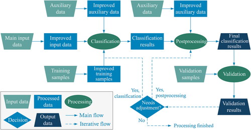
Wulder et al. (2018) identified seven elements of the land cover classification process: end-user needs (i.e., application area), defining land cover legend, gathering training and validation data, image preprocessing with the derivation of spectro-temporal metrics and incorporation of auxiliary data, classification with suitable algorithms, post-classification error mitigation with iterative accuracy assessment, and product delivery methods. Most of these elements are visible in Figure 2 and are further described in the following sections.

3.1. Defining classification legend

Land cover classification legend depends on the application area of a particular land cover product and end-user needs. When examining land cover products that do not focus on a specific application area (e.g., forestry), they usually classify the whole extent of the area that is being classified into dozen of classes that at least include: vegetated area, artificial (built-up) area, bare ground land, and water bodies. Some of these classes, especially one that refers to vegetated areas, are often divided into more classes (for example, high and low vegetation). As identified by Di Gregorio et al. (2016), many land cover products are produced with different objectives in mind, and the problematic part is establishing semantic interoperability between them. They also state that the most straightforward way of solving semantic inconsistency between different land cover products, which consists of comparing the class name and textual class descriptions, is time-consuming and ineffective. That is why Di Gregorio et al. (2016) created the FAO LCCS (short for Land Cover Classification System) classification system, i.e., a system that is intended for assigning objects to different classes (INSPIRE Thematic Working Group Land Cover 2013).

In the FAO LCCS, the emphasis is not on the standardization of classes but on the standardization of attribute terminology that is used to describe each class (Di Gregorio et al. 2016). It is used to create classification legends for different applications and to compare classes of different classifications. One of the aims of the FAO LCCS is to enable the automatic harmonization of different land cover products without the need for human intervention (Di Gregorio et al. 2016). International Organization for Standardization (ISO) in cooperation with FAO created the standard ISO 19144 Geographic information – Classification system that currently has two parts: ISO 19144-1 Classification system structure and ISO 19144-2 Land Cover Meta Language (LCML). LCML, which is expressed in Uniform Modeling Language (UML), allows describing different classification systems and comparing and integrating them (ISO 2012). Version 3 of the LCCS comes with a software application that is intended to be a tool for applying LCML concepts conveniently (Di Gregorio et al. 2016).

A similar aim, among others, in terms of enabling semantic comparison between different classification systems has the EAGLE concept (short for EIONET (European Environment Information and Observation Network) Action Group on Land monitoring in Europe; https://land.copernicus.eu/eagle). It is a tool that enables the interpretation of semantic information included in various land cover classes and translation between different classification systems (Zhu, Jin, and Gao 2021). EAGLE has also a goal of clearly separating land cover from land use information since they are both often included in the same classification legend (Arnold et al. 2021).

3.2. Input data and their preprocessing

All products that are analysed in this research use multispectral or multispectral and radar satellite images as a main source for extracting land cover information. Some products use many other auxiliary data sources to augment and possibly enhance the final product. One of the first steps would then be choosing data that will be used in producing land cover products and conducting preprocessing, i.e., preparing input data in a way that they are as useful as possible to extract land cover information from them.

Most multispectral satellite images are delivered in different levels of already preprocessed forms. In the case of Sentinel-2 images, two product levels are available to general users, level-1C (L1C) and level-2A (L2A). As further discussed in Section 3.2.1. Sentinel-2 mission, one of the main differences between Sentinel-2 L1C and L2A images is that L2A images are atmospherically corrected, meaning that pixel values correspond to surface reflectance (ESA 2015), i.e., they are more-less free from atmospheric influences. PROBA-V multispectral optical images used for the production of CGLS-LC100 were also preprocessed to generate surface reflectance from the TOA data (Buchhorn, Lesiv, et al. 2020). Radar data also require preprocessing, but a more complex one (Gašparović and Dobrinić 2020). However, their inclusion as input data in the land cover production might significantly increase classification accuracy (Venter and Sydenham 2021).

When optical images are used for classification, various spectral indices that are calculated from them are also commonly calculated and included as input data. Spectral indices, a common name for the vegetation, water, built-up, and soil indices (Rumora, Miler, and Medak 2020), when included as input for spectral classification, increase classification accuracy under some circumstances.

Some yearly land cover products use input data that are acquired throughout the whole year, which means there are numerous values for each pixel from different parts of the year. To take into account the phenological cycle of vegetation and thus increase classification accuracy, it is common to calculate the temporal metrics. For example, Venter and Sydenham (2021) calculated 5^th, 25^th, 50^th, 75^th, and 95^th percentile values for each pixel across all selected images within the year, as well as standard deviation, median NDVI values for summer, winter, spring, and fall and some other spectro-temporal metrics. Witjes et al. (2022) also used temporal metrics extracted from the Landsat data. They used seven spectral bands (blue, green, red, near-infrared (NIR), shortwave infrared 1 (SWIR1), SWIR2, and thermal), and divided them into three quantiles calculated for each month, and then from those data, they calculated different spectral indices. On the other hand, for the production of, for example, Dynamic World, single-date images were used. Dynamic World land cover products provide near real-time data but do not consider temporal characteristics of different land cover types. For instance, in one part of the year, some agricultural areas can be bare land, and others can be vegetated. Single date land cover product will in the corresponding part of the year classify those areas as bare land and in others as some of the vegetation classes. Suppose a user is interested in identifying land that is used for agriculture (which is more characteristic of land use than land cover) throughout the year, in general. In that case, it will be more accurately classified on products that use data from the whole year than just single-date data.

All the above metrics extracted from the input images are spectral, and they do not consider spatial relations between pixels. Some textural metrics can also be extracted and can indirectly include information from neighbouring pixels in the classification process. For example, it is possible to calculate a standard deviation of pixel values in a 5 × 5 moving window for a particular band or vegetation index (Venter and Sydenham 2021). Lower values in these layers with textural information point out to the pixels that are in homogeneous areas (surrounded by pixels with similar values), while higher values indicate more heterogeneous land cover (Buchhorn, Bertels, et al. 2020).

The following section focuses on sensors installed on satellites and used to acquire data used as main input data for conducting land cover classification. The analysis is limited only to sensors that are used to produce large-scale land cover products that are analysed in Chapter 2. Currently available global and continental land cover products. Those sensors are installed on Sentinel-1, Sentinel-2, Landsat, and PROBA-V satellites.

3.2.1. Sentinel-2 mission

Two Sentinel-2 satellites have been launched: Sentinel-2A in 2015 and Sentinel-2B in 2017 (Phiri et al. 2020). They are part of the space component of the Copernicus program, which is an Earth observation and monitoring program of the EU’s European Commission (Wiatr et al. 2016). ESA is in charge of the space component of the Copernicus program (Potin et al. 2015). Both Sentinel-2 satellites carry a passive sensor called a multispectral instrument (MSI) at an altitude of 786 km in an orbit that is sun-synchronous and are jointly providing global coverage of land and coastal sea with a 5-day revisit period (Gascon et al. 2017). The 5-day revisit period refers to equatorial areas and is lower towards the poles. Both Sentinel-2 satellites are orbiting in the same orbit but are on diametrically opposite sides.

MSI instrument is a push-broom sensor that is acquiring data in 13 spectral bands spreading over a visible, NIR, and SWIR range of the EM spectrum, with a spatial resolution of 10, 30, and 60 m (Gascon et al. 2017). Four bands have a spatial resolution of 10 m (blue, green, red, and one wider NIR band), six bands have a 20 m resolution (four narrow bands from the red-edge/NIR part of the spectrum, mainly for vegetation applications, and two wider bands from the SWIR part for detecting snow or clouds, assessing vegetation moisture, and similar applications), and three bands with a 60 m spatial resolution for conducting atmospheric corrections, detecting clouds and similar usages (Gascon et al. 2017).

There are three levels of Sentinel-2 products: level-0 (raw, compressed data), level-1, and level-2. Level-1 products are divided into level-1A (L1A), level-1B (L1B), and level-1C (L1C) products, while the only level-2 product is the level-2A (L2A) one. Level-1A products are decompressed level-0 products and are further radiometrically corrected to produce Level-1B products containing top-of-atmosphere (TOA) radiances (Gascon et al. 2017). Level-1C products are generated from level-1B ones, they contain TOA reflectance values, they are resampled to Universal Transverse Mercator (UTM) CRS, orthorectified, and are, unlike products from previous levels, publicly and freely accessible (Gascon et al. 2017). Level-2A products are produced from the level-1C products by converting TOA to the bottom-of-atmosphere (BOA) reflectance, thus minimizing atmospheric influences on the acquired data (Gascon et al. 2017). Sentinel-2 L2A tiles are accordant with minimal requirements of CARD4L-SR (short for CEOS (Committee on Earth Observation Satellites) analysis-ready data for land for surface reflectance products) specification (CEOS WGCV 2020a), meaning they can be analysed with minimal additional processing and should be interoperable with other CARD4L-SR datasets.

Some deficiencies of using Sentinel-2 images for generating land cover products are a lack of thermal bands and panchromatic band, uneven spatial resolution between bands, and also geolocational sensor-to-sensor misalignment with Landsat 8 images if they both want to be used in the same workflow (Phiri et al. 2020).

3.2.2. Sentinel-1 mission

Sentinel-1 mission is also a space component of the Copernicus program. Two Sentinel-1 satellites have been launched: Sentinel-1A in 2014 and Sentinel-1B in 2016 (Schubert et al. 2017). While Sentinel-1A is still fully operational, Sentinel-1B suffered an unrecoverable malfunction at the end of 2021 and ended its mission (ESA 2022a). To mitigate this loss, ESA announced speeding up the process of the Sentinel-1C satellite launch (ESA 2022a).

Sentinel-1 satellites are orbiting in a sun-synchronous orbit at 693 km altitude, they need 12 days to achieve global image coverage and are equipped with a C-band synthetic aperture radar (SAR) sensor (Geudtner et al. 2014; Schubert et al. 2017). Sentinel-1 satellites have four operational modes that provide different spatial resolutions and coverages: interferometric wide swath (IW, roughly 5 × 20 m resolution and 250 km wide swath), extra wide swath (EW, roughly 20 × 40 m resolution and 400 km wide swath), StripMap (SM, roughly 5 × 5 m resolution and 80 km wide swath), and Wave (WV, roughly 5 × 5 m resolution, 20 × 20 km scenes), which is the only mode that cannot operate in dual polarization (HH/HV or VV/VH; HH is short for horizontal transmit and horizontal receive, VH for vertical transmit and horizontal receive, and HV and VV analogously), but only in single (HH or VV; Geudtner et al. 2014; Miranda et al. 2017). Different imaging modes are utilized for different parts of the world, where IW and EW are the main imaging modes (Miranda et al. 2017). The observation scenario, which defines imaging modes that will be used for different parts of the world, is not constant and is changing based on observation requirements posed by the evolution of Copernicus services, requirements of ESA or EU member states, or by scientific or international initiatives (Potin et al. 2015).

Acquired data from each imaging mode are downlinked to the ground stations and processed to produce level-1, and level-2 products (Bourbigot, Harald, and Piantanida 2016). Level-1 products are slant range single look complex (SLC) and ground range, multi-look, detected (GRD), while level-2 are ocean (OCN) products that have three components: Ocean Swell Spectra (OSW), Ocean Wind Field (OWI), and Radial Velocity (RVL; Bourbigot, Harald, and Piantanida 2016).

OCN products, since they are mainly intended for applications on the sea, are not used as input data for land cover classification, while GRD Sentinel-1 images are. For example, for the production of ESA WorldCover and ELC-10 land cover products, GRD images were used as input data (Van De Kerchove et al. 2021; Venter and Sydenham 2021). SLC products are mostly not used for spectral-based classification. Some of the reasons are their more complex processing, multiple times bigger file sizes, and little additional useful information compared to GRD data (Hansen, Mitchard, and King 2020), however, there are also some examples of their utilization (Mohammadi et al. 2020). There are also examples of using SLC products for land cover classification based on polarimetric classification, and not on the spectral one, such as the one by Roychowdhury (2016). Roychowdhury (2016) classified urban areas into four broad classes (built-up, water bodies and wetlands, vegetation, and open spaces) and achieved higher overall accuracy with a polarimetric unsupervised classification of SLC data than with supervised and unsupervised spectral classification of GRD data.

GRD and SLC products both require preprocessing before they can be used and are not considered CEOS-ARD according to the CEOS WGCV (short for Working Group on Calibration and Validation) specifications. ESA does not currently provide CEOS-ARD for Sentinel-1, but a new product that will be following CARD4L-NRB (CEOS analysis ready data for land for normalized radar backscatter products) specification (CEOS WGCV 2021) is currently under development (ESA 2022b). However, ESA has provided the Sentinel Application Platform (SNAP), a free and open-source application that enables the processing of Sentinel-1 images, and also Sentinel-2 and Sentinel-3 ones (Weiß and Fincke 2022). Sentinel-1 images can be preprocessed with the Sentinel-1 toolbox (S1TBX) that is available in SNAP (Sumbul et al. 2021).

Mullissa et al. (2021) proposed a procedure for generating Sentinel-1 ARD on Google Earth Engine (GEE) from Sentinel-1 GRD scenes that are already preprocessed to a certain degree and available on GEE. Private company Sinergise offers a tool for generating CARD4L-NRB data from Sentinel-1 GRD images: Sentinel Hub CARD4L Generation Tool (Dyke et al. 2021). The tool is accessible at https://apps.sentinel-hub.com/s1-card4l/, but it is not freely available. Digital Earth Africa program partnered with Sinergise to produce the first continuously updating free and open continental CARD4L-NRB Sentinel-1 dataset available for Africa only (Yuan et al. 2022).

3.2.3. PROBA-V mission

PROBA-V satellite, equipped with VEGETATION (VGT) optical instrument and five other non-scientific instruments, was launched in 2013 (Wolters et al. 2018; ESA 2022c). In 2020, the VGT instrument ended its operational mission, but the PROBA-V satellite is still flying since other instruments remained operating (ESA 2021). The main objective of the PROBA-V mission was to ensure the continuity of the SPOT-VEGETATION mission until the launch of Sentinel-3 satellites (Wolters et al. 2018), which was more than fulfilled. PROBA-V satellite is flying in a sun-synchronous orbit at an altitude of 820 km (Wolters et al. 2018). VGT has four spectral bands including blue, red, NIR, and SWIR bands (Dierckx et al. 2014). It consists of three cameras that jointly provide 2-day global coverage, while the main camera that provides images with the highest spatial resolution ensures 5-day global coverage (Wolters et al. 2018). Spatial resolution is higher for the blue, red, and NIR bands and lower for the SWIR band, ranging at nadir from 100 to 180 m, and at swath edges, from 350 m to 660 m (Francois et al. (2014), as cited in Wolters et al. (2018)). PROBA-V products are available in three spatial resolutions: 100 m, 300 m, and 1 km; and in different product levels ranging from raw unprojected level-1C products to level-3 atmospherically corrected top-of-canopy (TOC) products (Wolters et al. 2018).

For producing CGLS-LC100, the complete level-1C data archive was reprocessed with enhanced atmospheric and a new geometric correction (Buchhorn et al. 2021). Generated TOC daily-synthesis data with a spatial resolution of 100 m were used as a primary source of earth observation (EO) data, and 300 m resolution images as a secondary one (Buchhorn et al. 2021).

3.2.4. Landsat program

The first moderate-resolution earth surface observations under the Landsat program were performed with the Landsat 1 satellite that was launched in 1972 (Markham et al. 2016). Ever since 1972, the Landsat program has been providing multispectral images with global coverage. The latest Landsat satellite, Landsat 9, which is a joint project of the National Aeronautics and Space Administration (NASA) and the United States Geological Survey (USGS), was launched in 2021 (Showstack 2022) and is almost a replica of its predecessor Landsat 8 that was launched in 2013 (Markham et al. 2016). Landsat 8 satellite was the first one of the Landsat satellites that was equipped with push-broom instruments (Markham et al. 2019), while previous ones were equipped with whisk-broom ones (Barsi et al. 2016).

Landsat 9 carries the second Operational Land Imager (OLI-2) and second Thermal Infrared Sensor (TIRS-2), and they have almost the same characteristics as OLI and TIRS instruments onboard Landsat 8 (Markham et al. 2019). OLI and OLI-2 observe the surface of the Earth in nine spectral bands: three from the visible part of the spectrum that corresponds to the red, green, and blue wavelengths, one from NIR and two from SWIR parts of the spectrum, ‘cirrus’ band, ‘coastal aerosol’ band, and one panchromatic that covers almost the entire visible part of the spectrum (Markham et al. 2019). All OLI and OLI-2 bands have a spatial resolution of 30 m, except the panchromatic band, which has a 15 m resolution (Markham et al. 2019). TIRS-2 is a more reliable version of the TIRS instrument, with eliminated performance problems that were noticed on TIRS (Markham et al. 2016). TIRS and TIRS-2 instruments have two bands covering the thermal infrared part of the spectrum and have a 100 m spatial resolution (Markham et al. 2019).

Landsat 4-9 satellites are deployed in a sun-synchronous orbit at an altitude of 705 km (Masek et al. 2020; NASA 2021). Landsat 8 and 9, currently only operational Landsat satellites (Markham et al. 2016; Landsat 7 ended its nominal science mission in April 2022 (USGS 2022b)) need 16 days to capture the entire surface of the Earth with OLI and TIRS instruments (Masek et al. 2020). Landsat 9 satellite, which took the place of Landsat 7, is shifted in phase by 8 days from Landsat 8 and is thus jointly with Landsat 8 providing global coverage every eight days (Masek et al. 2020).

The USGS is distributing Landsat images after conducting various types of processing. In 2016 all Landsat images were reprocessed into the so-called collection-1 dataset in order to ensure that images are suitable for time-series analysis and compositing (USGS 2019). All collection-1 products were removed from the USGS archives and are not accessible through USGS platforms as of the end of 2022 (USGS 2022a). The entire Landsat archive was again reprocessed using consistent radiometric and geometric algorithms to the collection-2 dataset that became available in late 2020 (Choate et al. 2021). One of the main reasons for producing the collection-2 dataset is to improve its geolocation accuracy (Dwyer et al. 2018) and harmonize Landsat and Sentinel-2 missions by improving their pixel-based positional alignment (Masek et al. 2020. Harmonization between Sentinel-2 and Landsat 8/9 data is particularly interesting because they jointly provide a global average median revisit interval for all four sensors (MSI on Sentinel-2A and Sentinel-2B, OLI, and OLI-2) of 2.3 days (Li and Chen 2020). Collection-2 consists of level-1 (TOA reflectance for complete Landsat archive) and level-2 (surface reflectance and surface temperature for Landsat 4-9) products that are divided into so-called tier-1 and tier-2 categories (USGS 2021). Images are placed in the tier-1 category if their geometric root-mean-square triangulation error (RMSE) is below 12 m and in tier-2 otherwise (Masek et al. 2020). Collection-2 is being continuously updated with new Landsat 8 and Landsat 9 data as they are being acquired (USGS 2021).

Collection-2 level-2 images are ARD products that are compliant with CARD4L-SR and CARD4L-ST (CEOS analysis-ready data for land for surface temperature products) specifications (CEOS WGCV 2020a, 2020b). USGS is also delivering the so-called U.S. ARD for Conterminous United States (CONUS), Hawaii, and Alaska from the Landsat 4-9 level-1 images (Dwyer et al. 2018; USGS 2022c). Another already mentioned global surface reflectance Landsat ARD (but not a CEOS-ARD) dataset is being produced by the GLAD from Landsat data acquired from 1997 to the present (Potapov et al. 2020). These GLAD Landsat ARD images were used to produce ODSE-LULC land cover product.

3.3. Auxiliary data

Auxiliary data can be used as input for classification, along with optical and/or radar data, or they can be used to enhance classification accuracy after classification was performed. For example, in the production of ESA WorldCover, altitude and slope extracted from the digital elevation model were used as additional features included in the classification phase, while OpenStreetMap and GHSL data, among others, were used as a support in making the final decision on land cover class for each pixel (Van De Kerchove et al. 2021).

Auxiliary data often need certain preprocessing before they can be included in some of the phases of creating land cover products. Some of that preprocessing include rasterizing vector data, reprojecting data to the common CRS, extracting only a useful subset of data, harmonizing different classification schemes, etc. Including auxiliary data can greatly improve classification accuracy, as shown by Venter and Sydenham (2021). Khatami et al. (2016) also showed that the inclusion of auxiliary data could significantly increase classification accuracy, much more than including spectral indices.

3.4. Training and validation samples

Almost all currently used land cover classification techniques are supervised, meaning they are heavily dependent on an often large volume of training data. Those data are used to train the classification algorithm, which then classifies the so-called never-before-seen data in the corresponding class. To validate classification results, an additional validation dataset is also required. The validation dataset is most often acquired at the same time as the training one but is not used in the training phase. Wulder et al. (2018) state that training and validation data can be acquired by in-situ sampling, by creating samples using higher resolution aerial or satellite images, from pre-existing suitable non-remote sensing data, from other available land cover data, and more recently, by exploiting volunteered geographic information (VGI), or more advanced techniques including adaptive based learning.

Currently, training and validation samples are most often acquired by assigning a land cover class to each pixel by making a comparison to adequate higher spatial resolution remote sensing images. The process of creating a completely new training and validation dataset this way, because it is often almost entirely manual, is the most time-consuming step in the land cover production workflow. The quality and design of the sampling procedure are often directly correlated with the overall classification accuracy.

In some cases, already existing datasets are used for training and validation. The obstacle that often needs to be overcome in this case is an incompatibility between the classification scheme used in the production of particular existing training datasets and the scheme defined for a land cover product that should be created based on that dataset. One example of a dataset that was not primarily created for training and validation of land cover classification products (d’Andrimont et al. 2021), but is becoming increasingly used for it, is the Land Use/Cover Area frame Survey (LUCAS) data. LUCAS land cover and land use statistical data are collected by in situ surveys that are cyclically repeated within the EU countries every three years since 2006 (d’Andrimont et al. 2021). Before 2018, LUCAS data were collected and delivered in the form of points with assigned, among other data, land cover and land use information. The dataset from 2018, unlike previous ones, additionally contains the so-called LUCAS Copernicus module, which is specifically designed to be suitable for EO applications (d’Andrimont et al. 2021).

Another example of using existing land cover products is applied in the production of S2GLC. As already mentioned, HRLs and CLC were used as data sources for generating training samples. Training samples were generated by applying a set of rules on HRLs, CLC, and indices extracted from Sentinel-2 images for each of the 13 land cover classes (Malinowski et al. 2020). Those rules, which can be fully automated, were applied to a couple of Sentinel-2 images, and then up to 1000 training samples for each land cover class were randomly extracted (Malinowski et al. 2020). Finally, as Malinowski et al. (2020) explain, those samples were used to classify each previously selected Sentinel-2 image from 2017 with an RF classifier. Although it can be fully automated, this classification workflow can also be considered a supervised one since it uses a classifier that requires a training dataset. The difference between this workflow and classical supervised classification is that the training dataset is not acquired manually but automatically.

Recently, a couple of datasets for training deep learning models for land cover classification have become available. Helber et al. (2017) created a dataset consisting of 27,000 labelled Sentinel-2 patches that are suitable for DL scene-based land cover classification (available at https://zenodo.org/record/7711810#.ZAm3k-zMKEA). Sumbul et al. (2021) generated the BigEarthNet-MM dataset that contains more than 590,000 pairs of Sentinel-1 and Sentinel-2 patches from 10 European countries, also for scene-based DL studies (available at https://bigearth.net/). Benhammou et al. (2022) provided Sentinel2GlobalLULC, a global Sentinel-2-based dataset, again for scene-based land cover classification (available at https://zenodo.org/record/6941662). The dataset that is also freely available and is suitable for pixel-based DL land cover classification is a dataset that was used for creating Dynamic World land cover product (provided by Tait et al. (2021)).

When considering training and validation samples, the Geo-Wiki platform (available at https://www.geo-wiki.org/) should also be mentioned. Although the Geo-Wiki platform now provides many different applications, the main one is still the Geo-Wiki application that is used for crowdsourcing training, calibration, and validation data for producing land cover datasets (S. Fritz et al. 2012). Fritz et al. (2017) combined data collected via the Geo-Wiki application from four campaigns and created a single land cover and land use dataset for the validation and training phase of producing land cover maps.

The Geo-Wiki app was used in the production workflow of CGLS-LC100 (Buchhorn, Lesiv, et al. 2020) and ESA WorldCover (Tsendbazar, Li, et al. 2021). In the production of the training dataset for the Dynamic World land cover product, the Labelbox platform (available at https://labelbox.com/) was used as a tool for drawing vector polygons, i.e., annotating land cover classes on Sentinel-2 tiles for deep learning classification (Brown et al. 2022).

3.5. Land cover classification

Classification is, in this sense, a process of determining the most probable land cover class for each pixel. This research is mostly limited only to the pixel-based supervised classification which uses spectral information acquired by multispectral sensors as a main input data source. Classification is carried out in the so-called feature space, where each pixel corresponds to one point whose coordinates are determined by feature values assigned to that pixel. Features are variables that are used as input for classification and are assigned to each pixel, such as bands from multispectral images, vegetation indices extracted from them, auxiliary data, and all other data that should help distinguish different land cover classes. Originally, only bands from multispectral images were used for classification since it is expected that similar land cover should have similar spectral characteristics (i.e., they should similarly interact with electromagnetic (EM) waves). Additional features that are included in classification should also follow that principle: similar land cover should have similar ‘behaviour’ for a particular feature. Dimensions of feature space are equal to the number of features. It is expected that points in feature space corresponding to a single land cover class should be relatively close to each other. The classification algorithm has a task to determine the delineation between classes in feature space and then assign a class to every point, and consequently to every pixel. To delineate classes, a supervised classification algorithm requires a training dataset that consists of pixels, i.e., corresponding points in feature space for which land cover class is already determined.

As already stated, this paper limits research to pixel-based supervised classification. This kind of satellite image classification is inductive (Raiyani et al. 2021), meaning that it is based on drawing conclusions for the whole dataset from just one subsample of it. As already discussed although there are other classification techniques, such as GEOBIA which shows a tendency to achieve high classification accuracy and unsupervised algorithms, pixel-based supervised classification techniques are still the most widely used ones (Phiri et al. 2020), especially for producing large-scale land cover products that are based on moderate resolution remote sensing images. There are multiple classification algorithms, some of which are mentioned in the following section.

3.5.1. Classification algorithms

The two most often used metrics to compare classification algorithms (i.e., classifiers) are classification accuracy and the time needed for performing classification. When comparing classification algorithms based on these two metrics, it should be ensured that all other variables that influence accuracy and processing time remain unchanged. This for example means that input data and training and validation datasets remain unchanged. Many papers have been comparing different classifiers for land cover classification on satellite images, some of which are mentioned below.

Khatami et al. (2016) found that different studies report disagreeing results concerning achieved accuracies with different classifiers which provoked them to make further investigation and to draw some general conclusions. They did not limit their research only to the influence of classification algorithm choice on classification accuracy but also to preprocessing methods applied to input data. Meta-analysis was run on 157 peer-reviewed articles by pairwise comparing overall accuracies achieved by different classifiers, with a drawback that it included only articles published before 2012 (Khatami, Mountrakis, and Stehman 2016). That is rather outdated, but some meaningful insights can be drawn out. Based on a meta-analysis, Khatami et al. (2016) concluded that Support Vector Machines (SVM) classifier outperformed the Maximum Likelihood classifier (MLC) in 28 out of 30 studies and the Neural Network algorithm in 14 out of 22 studies with a tendency to have a better performance when spatial and spectral resolutions are higher. SVM also achieved higher overall accuracy (OA) than the Random Forest (RF) classifier. Another finding is that K-Nearest Neighbor, although a very simple algorithm, slightly outperformed MLC in 12 out of 17 studies (Khatami, Mountrakis, and Stehman 2016).

Phiri et al. (2020) investigated the findings of multiple articles concerning the usage of Sentinel-2 images for land cover mapping, including the comparison of different algorithms used for that purpose. They found out that machine learning (ML) algorithms dominate, including RF, KNN, SVM, and Bayes, and more sophisticated Convolutional Neural Networks (CNN). It is interesting to notice that most of the land cover products that are listed in Table 1 were produced by a random forest classifier, which supports the conclusion of Phiri et al. (2020) which denotes it as the most commonly used classifier.

Many researchers investigated land cover classification accuracies using different classifiers but within a limited geographical area. This is one of the problems identified by Small (2021), stating that in many articles, it is not clear if the methodology being developed is suitable for general application or just in the area in which it was applied. Nevertheless, these articles can be a valuable source of information when choosing which classifier should be applied.

Talukdar et al. (2020) examined land cover classification accuracies for six machine learning algorithms, specifically Artificial Neural Network (ANN), RF, Fuzzy Adaptive Resonance Theory-Supervised Predictive Mapping (Fuzzy ARTMAP), SVM, Spectral Angle Mapper (SAM), and Mahalanobis distance (MD). The classification was performed on Landsat 8 images with a conclusion that, although no major classification accuracy differences were obtained between all used classifiers, the highest accuracies were achieved with RF, ANN, and SVM, in that order, from the most accurate one (Talukdar et al. 2020). Talukdar et al. (2020) also list a dozen of research that dealt with the comparison of classification accuracies achieved by different classifiers and concluded that in most papers RF, ANN, and SVM were reported as the most accurate classifiers. Finally, Talukdar et al. (2020) point out that the analysis of classifier accuracies in different climatic regions still has to be done.

Artificial Neural Network (ANN) is a non-parametric classification technique (Talukdar et al. 2020), meaning that it does not presume the nature of data distribution (Vali, Comai, and Matteucci 2020). The ANN is constructed in a similar way to the human nervous system, it consists of connected nerve fibres (Talukdar et al. 2020). One of the advantages of the ANN classifier is its ability to generate useful results even if training data are incomplete or erroneous. The ANN contains three types of layers: the input layer in which each node represents one feature in a dataset that has to be classified (for example, each spectral band or auxiliary dataset), the output layer, in which each node corresponds to one class, and hidden layers that is between those two layers and that consists of a user-defined number of layers and nodes within them (Shih, Stow, and Tsai 2019). In general, nodes from the input layer are connected with nodes in the hidden layer which are connected with nodes in the output layer. Weight is assigned to each connection and that weight is being adjusted in the training phase. In the training phase, for pixels that have known both, input and output values, weights of connections are being adjusted so that most of the training samples are correctly classified in the appropriate class, i.e., so that discrepancies between network-generated classes and classes assigned to training samples are minimized (Shih, Stow, and Tsai 2019; Talukdar et al. 2020). When ANN is trained, it can be used to classify new data in corresponding classes. Two main parameters that have to be defined by the user are the learning rate (i.e., the amount of weight change in each iteration) and the number of iterations (Shih, Stow, and Tsai 2019). Both parameters influence the classification accuracy and the best way to define their optimal values is to apply a trial-and-error approach (Talukdar et al. 2020).

Support Vector Machines (SVM), which is also a non-parametric method (Talukdar et al. 2020), applies a more traditional approach by delineating classes in feature space. The training dataset is used to determine hyperplanes that separate one class from another (Shih, Stow, and Tsai 2019). The user has to define two hyperparameters: C and gamma (Talukdar et al. 2020). The value of the C hyperparameter has to be carefully chosen since the wrong value can lead to model overfitting or underfitting because it presents a compromise between class separation and training error (Rumora, Miler, and Medak 2020). The gamma hyperparameter controls the shape of the hyperplanes and in that way affects the obtained accuracy.

Random Forest (RF), also a non-parametric algorithm (Talukdar et al. 2020), is a machine learning method that is based on Decision Trees (DT; Masiliūnas et al. 2021) and that was developed by Breiman (2001). RF model requires two main parameters: the number of trees and the number of features that, when reached, will initiate a split in DT (Malinowski et al. 2020). Random forest algorithm is also considered an ensemble-based machine learning algorithm in which each tree in the forest gives a vote on class and the final class is determined based on the majority of votes from all trees (Shih, Stow, and Tsai 2019; Talukdar et al. 2020). RF is more immune to overfitting and errors in training samples than other algorithms are (Malinowski et al. 2020). Burgueño et al. (2023) compared ANN and RF algorithms and found that RF yields better results because it better classifies spectrally heterogeneous classes.

3.6. Validation of land cover products

For a land cover product to be useful to the end user, it is required to provide convenient information about its quality. Validation of land cover products is a necessary part of the production process. Its importance is affirmed by the fact that two documents usually accompany most land cover products: one describing production workflow and communicating general information about the land cover product, and another reporting validation results.

Validation is mostly done by comparing classification results with the validation dataset. The validation dataset is usually acquired in the same way as the training dataset with the main difference being that the validation dataset is not used for training the classifier. In any case, the validation dataset must have an accuracy much higher than the expected accuracy of the land cover product. By comparing classification results, i.e., land cover classes that are assigned to pixels, with the validation dataset (considered true data), it is possible to calculate different measures that report classification quality. The metric that is most often used and that is easy to calculate is overall accuracy. Overall accuracy reports the percentage of correctly classified pixels from all pixels included in a validation dataset.

CEOS WGCV Land Product Validation (LPV) Subgroup has a mission to standardize quantitative validation of products (not only land cover ones) derived from different satellite sensors and obtained by different algorithms (CEOS WGCV LPV Subgroup 2022). CEOS WGCV LPV Subgroup defines five validation stages, where each stage has more restrictive requirements than its predecessor (CEOS WGCV LPV Subgroup 2022). Stage-0 does not require any validation, while stage-1 requires accuracy assessment on not more than 30 locations and time periods (CEOS WGCV LPV Subgroup 2022). For stage-2, it is necessary to conduct accuracy estimation with a validation dataset including more than 30 spatiotemporal locations and to assess spatiotemporal product consistency and consistency with other similar products (CEOS WGCV LPV Subgroup 2022). In addition to the requirements of stage-2, stage-3 requires that validation assessment is quantitively expressed and based on procedures that are well acquainted amongst the validation community (CEOS WGCV LPV Subgroup 2022). Finally, stage-4 requires that whenever a new version of the product or a new iteration for time series products is available, stage-3 results for a particular product are systematically updated (CEOS WGCV LPV Subgroup 2022).

Strahler et al. (2006) identified five components of the validation process: (1) obtaining statistical measures of accuracy and their variances, (2) generating confidence maps in which each pixel has a value that corresponds to classification confidence based on the training dataset, (3) comparison between generated land cover product and other comparable land cover datasets, (4) qualitative accuracy review by dividing the land cover product into regular regions and assessing its quality by, for example, comparison with imagery of higher spatial resolution, other available datasets and expert assessment, and (5) validation of land cover change, which poses a significant problem because it requires comparison of two different land cover products, each of which has its own classification uncertainties. Regarding the last component, Tsendbazar, Herold, et al. (2021) state that the continuity of global land cover maps through the years is an essential requirement for monitoring global land-related issues, but that the temporal stability of those maps is rarely assessed. They have therefore focused their research on the validation of annual land cover maps with an emphasis on evaluating temporal consistency and thus providing a framework for conducting validation that is in line with CEOS WGCV LPV stage-4 requirements. Strahler et al. (2006) also emphasize three validation outputs that should be reported with each land cover product to communicate its quality effectively: (1) overall single value that provides insight into the accuracy of land cover product with its confidence interval, (2) class-wise accuracies, and (3) per-region (country, continent, etc.) accuracy measurements, especially for global land cover products (Strahler et al. 2006).

3.7. Georeferencing large-scale land cover products

Although georeferencing land cover products cannot be considered as a separate step within the land cover map production workflow since it is for the most part imposed by the producers of the input data, there are some challenging aspects related to georeferencing global datasets that are discussed below.

Projection of each imaging sensor element (i.e., each element in the push-broom sensor) onboard satellite through imaging optics and on the surface of the Earth is called an instantaneous geometric field of view (IGFOV; Joseph 2020) or ground projected instantaneous field of view (GIFOV; Markham et al. 2020). A similar term is the ground sampling distance (GSD), but it can be different from IGFOV if the satellite image producer has done certain resampling and it thus represents a distance between pixel centres on the ground (Joseph 2020). These observations acquired by sensors on EO satellites are delivered in raster formats, and the same is usually true for land cover products generated from them. Representing global datasets, or sometimes even regional and continental ones, in raster format poses a challenge.

There are two broad options to choose from when it comes to choosing how to georeference global raster dataset: data can be either georeferenced in the so-called geographic coordinate reference system (CRS) where latitude and longitude are used for defining the location of a raster or projected CRS can be used where cartographic projection defines a transformation from the curved surface of the ellipsoid to the cartographic projection plane. Both approaches have advantages and disadvantages. In the geographic coordinate reference system, coordinates are expressed in angular units, while in projected CRS in linear units. This might be characterized as a drawback for geographic CRS when it is needed to calculate distances and areas, but it should not be since modern GIS applications allow conducting calculations on the surface of the ellipsoid (Frančula et al. 2021). On the other hand, calculating distances and areas from data georeferenced in projected CRS is simpler since calculations are planar, but choosing the right projection can be problematic because of inevitable deformations introduced by map projections. For global raster datasets that are mostly used for areal calculations, a projection that does not deform areas (i.e., equal-area projection) should be used (Steinwand, Hutchinson, and Snyder 1995). Examples of equal area projections are the Albers Equal Area Conic projection that is used for U.S. ARD Landsat data (Dwyer et al. 2018), Lambert Azimuthal Equal Area (LAEA) projection that is recommended for pan-European areal spatial analysis (INSPIRE Thematic Working Group Coordinate Reference Systems & Geographical Grid Systems 2014) and Sinusoidal projection used for Moderate Resolution Imaging Spectroradiometer (MODIS) land cover products (Sulla-Menashe and Friedl 2018). Moreira de Sousa, Poggio, and Kempen (2019) compared five equal-area projections that are available in free and open-source software for geospatial processing and concluded that Homolosine projection is the most suitable in terms of lowest angular and linear distortions, while Sinusoidal one introduces too large distortions (as cited by Kmoch, Vasilyev, et al.(2022)).

It is interesting to notice that Sentinel-2 level-1C, and level-2A, as well as Landsat collection 2 level-2 images, are provided in Universal Transverse Mercator (UTM) projection (Gascon et al. 2017; Dwyer et al. 2018). UTM projection introduces linear deformations that are negligible for most applications, but a drawback is that UTM imposes 60 CRSs, each for every 6° longitude UTM zone. This makes using UTM somewhat challenging since global data are not continuously georeferenced.

When geographic CRS is used for georeferencing global raster data, the problem arises from the fact that the distance between two meridians on the surface of the ellipsoid in the east-west direction is not constant. For example, the distance between two meridians that are 1” apart (i.e., that have longitudes that differ for 1”) on the surface of the WGS84 ellipsoid is around 30 m at the equator and it decreases towards poles, where it reaches 0 m. This is not a problem in the north-south direction because a meridian is almost a circle on ellipsoids that are used as an approximation of the Earth’s surface, so a single central angle always corresponds to almost the same length on the meridian. Since pixels are rectangular and have a constant dimension within a single raster (corresponding to the constant longitude and latitude span), it means that each pixel does not correspond to the same area on the surface of the ellipsoid. On the other hand, conditionally said, GIFOV has a constant dimension. One of the approaches to mitigate this issue is to define a raster so that its resolution (i.e., pixel size) at the equator corresponds to the dimensions of the GIFOV. That way, at the equator, each IGFOV will be mapped to one pixel and to multiple pixels by going poleward. A more sophisticated solution that reduces redundancy, introduced by mapping a single GIFOV to multiple pixels, is to define latitude zones where different resolutions (i.e., pixel dimensions) are assigned to different zones. This approach is applied to some digital elevation models (DEM) georeferenced in geographic CRS, such as CopernicusDEM (https://doi.org/10.5270/ESA-c5d3d65). Defense Gridded Elevation Data (DGED; Defense Geospatial Information Working Group 2020) and Digital Terrain Elevation Data (DTED; U.S. Department of Defense 1996) are two specifications/standards that define these longitudinal zones and corresponding resolutions. For example, DTED defines 0° − 50°, 50° − 70°, 70° − 75°, 75° − 80°, and 80° − 90° latitude zones with pixel sizes in east-west direction of 1”, 2”, 3”, 4”, and 6” respectively, while pixel size in meridian direction (north-south) is constant for all zones and is 1” (U.S. Department of Defense 1996). A disadvantage of this approach is similar to the disadvantage of the UTM, with the difference that zones are now latitude and not longitude ones.

One solution that is particularly suitable for storing observations made by sensors on EO satellites that have a constant GIFOV and for storing any global raster dataset is using a so-called discrete global grid system (DGGS). In essence, DGGS tessellates the ellipsoid’s surface in regular equal-area grid cells (OGC 2021) and does not necessarily project them into a map projection plane. The problem with DGGS is that it is far from being widely implemented and accepted within the GIS community, although some authors (Kmoch, Matsibora, et al. 2022) believe that is about to change.

3.7.1. Reprojecting raster data

Reprojecting raster data means changing CRS in which the raster is georeferenced. Since pixels are defined by lines that are perpendicular to the axes of the coordinate system, when CRS changes, resampling needs to be done. Different resampling methods are in use, but each of them alters the original data in one way or another. Nearest neighboured resampling spatially shifts original pixels for up to a half dimension of the pixel but preserves original pixel values, while bilinear and cubic convolution resampling can smooth data, which can be beneficial in some applications, but they alter original pixel values (Dwyer et al. 2018). One problem that can happen in this process, which is especially problematic with EO data, is pixel loss and replication (White 2006; Moreira de Sousa, Poggio, and Kempen 2019).

During the production of the Landsat U.S. ARD images that are georeferenced in Albers Equal Area Conic projection referenced to the WGS84 datum, raw Landsat data were directly used, instead of collection-1 or collection-2 data (Dwyer et al. 2018). Collection-1/collection-2 data are georeferenced in the UTM projection referenced to the WGS84 ellipsoid, which means that if those data were used, reprojection would be done twice (Dwyer et al. 2018). Since Sentinel-2 data are delivered in UTM CRS, when the area of interest spans for more than 6° in an east-west direction, there is usually a need to reproject Sentinel-2 images to one common coordinate reference system. This is especially problematic on edges between adjacent UTM zones because of overlapping between Sentinel-2 images. Roy et al. (2016) focused their research on best practices for resampling and reprojecting Sentinel-2 images with an emphasis on reprojecting overlapping parts of images from different UTM zones.

4. Discussion

When comparing the six land cover products that are described in Chapter 2. Currently available global and continental land cover products, differences, some of which are quite significant, can be observed regarding their characteristics, such as used input data, achieved accuracies, number of land cover classes, and utilized classification algorithms. There are also similarities, especially in the general steps of the production workflow which are shared among all of the analysed products. This chapter discusses and compares characteristics of six analysed recent land cover products and identifies some of the challenges that are present in different steps of the land cover map production workflow.

Regarding the main input data, since large-scale land cover mapping is in focus, coarse to moderate spatial resolution satellite images were used as a main data source for land cover classification, namely Sentinel-1, Sentinel-2, Landsat, and PROBA-V images. All these images are freely available and therefore heavily utilized not only for producing land cover maps but also for other applications. Higher-resolution images (higher than 10 m spatial resolution) are still not freely available, but it is questionable if their usage for large-scale geographical area analysis would even be feasible. All analysed products, instead of ESA WorldCover and ELC10 have been using optical satellite images (Sentinel-2, Landsat, PROBA-V), while these two products were additionally using Sentinel-1 SAR images. During the production of ELC10, Venter and Sydenham (2021) compared classification accuracy when using only Sentinel-1, only Sentinel-2, and both, Sentinel-1 and Sentinel-2 images. They have concluded that fusion of radar (Sentinel-1) and optical (Sentinel-2) data significantly improves accuracy as compared to when only optical or radar data are used. A similar conclusion concerning the fusion of Sentinel-1 and Sentinel-2 data was raised by Phiri et al. (2020). Phiri et al. (2020) also concluded that due to higher spatial resolution overall classification accuracy is higher when using Sentinel-2 images than when using Landsat ones. On the other hand, the immense advantage of Landsat data is their long temporal availability which makes them a great choice when performing long-term land cover analysis. That is the reason why ODSE-LULC has the longest temporal coverage as compared to other analysed land cover maps.

As already stated, optical and radar data have to go through some levels of preprocessing before they can be used for producing land cover maps. In the case of Sentinel-1, Sentinel-2, Landsat and PROBA-V satellite images, they are already available in forms that are a result of different processing stages. However, some further preprocessing is in some cases still needed. Regular preprocessing step for optical images include conducting atmospheric correction. However, in research that was conducted by Rumora et al. (2020) and Venter and Sydenham (2021), it was shown that atmospheric correction has a minimal influence on the overall classification accuracy and can therefore be omitted. In other words, it seems that there is no significant difference in classification accuracy between cases when using Sentinel-2 L1C and L2A images. In terms of radar images preprocessing, Venter and Sydenham (2021) found that speckle filtering, a regular step in radar data processing, does not significantly improve classification accuracy and can be skipped. The authors themselves emphasize that more research is needed to confirm this finding.

When comparing other input data (Table 1) that are extracted from the optical and/or radar data, it can be observed that for producing different analysed land cover products different spectral indices, as well as temporal and textural features were used. Witjes et al. (2022) and Venter and Sydenham (2021) found spectral indices, such as NDVI, NBR, and NBR2, as being among the most influential features on land cover classification results. On the other hand, in an analysis conducted by Burgueño et al. (2023) slope derived from DEM was indicated as the most important variable in classifying land cover on the coast of the Mediterranean basin using an RF classifier. Rumora et al. (2020) showed that for single-date images, an RF classifier has higher accuracy when spectral indices are included than when they are not. Along with spectral indices, temporal features can also be extracted from the optical data and thus temporal characteristics of a particular land cover can be included in the classification process. For example, Witjes et al. (2022) for producing yearly ODSE-LULC land cover maps used Landsat reflectance values from different seasons throughout the year and in that way, they directly included temporal variability in different land cover classes. For producing ELC10, Venter and Sydenham (2021) calculated the per-pixel standard deviation of the reflectance values from time-series Sentinel-2 images, which is an example of how temporal characteristics can be indirectly included. Along with spectral indices and temporal features, textural features can also be included in pixel-based land cover classification. Khatami et al. (2016) reviewed multiple articles dealing with the inclusion of various input data in the classification process and concluded that including texture information leads to the highest improvements in achieved classification accuracies as compared to other input data they analysed. For ELC10 per-pixel standard deviation of seasonal median NDVI values in a 5 × 5 moving window was calculated (Venter and Sydenham 2021), and for CGLS-LC100, the standard deviation was calculated from yearly time-series data for a 3 × 3 pixels moving window (Buchhorn, Bertels, et al. 2020). In this way, spatial characteristics of a particular land cover class were also indirectly included in the classification process.

Concerning other auxiliary data that are listed in Table 1 and are used in land cover production workflow, either as one of the features in the classification process or as auxiliary data for postprocessing, some interesting findings can be emphasised. As stated and proved by Venter and Sydenham (2021), including auxiliary features can drastically improve classification results when producing a large-scale land cover map, especially for particular classes that have different spectral characteristics in different regions. Among auxiliary data, most often are used terrain characteristics such as height, slope, and aspect were derived from various digital elevation models (DEM). It is interesting to notice that ELC10 and ODSE-LULC used night light images from the Visible Infrared Imaging Radiometer Suite (VIIRS) Day/Night Band (DNB; H. Chen et al. 2017) and that for producing ELC10 precipitation and temperature data were used from the European Centre for Medium-Range Weather Forecasts (ECMWF) Reanalysis v5 (ERA5). On the other hand, for the Dynamic World land cover product, classification is performed only on Sentinel-2 images, without auxiliary data. Auxiliary data were used only during training data collection (Brown et al. 2022).

By comparing datasets that were used for training the classification algorithms for each of the analysed land cover products, it can be observed that for CGLS-LC100, ESA WorldCover, and Dynamic World land cover products, those datasets were manually collected, while for ELC10, S2GLC, and ODSE-LULC they have been extracted from already available datasets. For ELC10 and ODSE-LULC training data were extracted from the LUCAS database, and for S2GLC they have been extracted from the CORINE land cover product and Copernicus high-resolution layers (HLS; Malinowski et al. 2020). An interesting finding by Malinowski et al. (2020) is that even if the data source used for the training phase has a lower resolution and is outdated, the classification results are still suitable for accurate classification. A similar remark in terms of the possibility of using training data from one year to classify images from another year was pointed out by Burgueño et al. (2023).

Regarding the classification algorithm, except for ESA WorldCover and Dynamic World, the RF classifier is the most often used one among the analysed products. For ESA WorldCover, the CatBoost algorithm was used and for Dynamic World a deep learning FCNN one. For ODSE-LULC, RF was used along with gradient boosted trees, and a neural network in an ensemble of machine learning classifiers. Most of these algorithms were used in a way that allowed the production not only of a discrete classification map but also a corresponding probability map. For example, the Dynamic World product provides per-pixel class probabilities for each of the eight classes and thus provide users greater flexibility in creating specific discrete classification map that best fits their needs by applying different thresholds to their values (Brown et al. 2022). Even more data regarding probabilities are provided with ODSE-LULC data. Since each of the three utilized classification algorithms provided per-class probabilities, the final probability was calculated for each pixel and also a corresponding standard deviation that provides insight into the reliability of the classification (Witjes et al. 2022).

When comparing classes and classification systems that are used for generating analysed land cover products, it can be observed that most of the products classify land cover into 8 to 13 classes, except ODSE-LULC which classifies them into 43 CLC classes and CGLS-LC100 which classifies them into 22 classes. There are no notable differences between the scope of the classes for different products, only it can be mentioned that CGLS-LC100 has 12 different classes for distinct types of forests. Along with the six land cover products that are analysed in this paper, there are many other available global, continental, and regional land cover products, and the idea of integrating multiple data sources to generate another product that should have higher reliability and accuracy is very tempting. The main challenge in this process is the fact that different land cover products use different classification systems (i.e., different class definitions) that are not easily comparable. Although some tools are developed to solve this issue, such as FAO LCCS, this is still a complex process that is sometimes impossible to perform.

From both, a user’s and producer’s point of view, the results of the last step in the production workflow (i.e., validation) are of great importance. For users, validation results will determine if a particular land cover product can be used to generate derived data with the desired accuracy. For producers, validation is important for determining their products’ quality and identifying problematic production steps that should be improved. Land cover products are often used for land cover monitoring. As pointed out by Tsendbazar, Herold, et al. (2021) for that kind of land cover analysis, it is crucial to ensure temporal consistency and stability in accuracy between yearly land cover products. In other words, there should be some kind of enforcement to ensure temporal consistency between yearly, or seasonal land cover maps (a good example is a quite complex procedure employed for this purpose in the production of CGLS-LC100). However, currently available global land cover products that are delivered as yearly time-series products do not report accuracies for each yearly instance but rather for the whole time-series (Tsendbazar, Herold, et al. 2021). When comparing different land cover products in terms of their thematic accuracy, there are challenges in metrics that are used to report thematic accuracy. Although many metrics have been developed, it is not always the case that the same metric is being used to report the quality of multiple land cover products which makes those products hardly comparable. The kappa coefficient, which is still widely used for reporting classification accuracy, is proven to be misleading (Pontius and Millones 2011). Since different validation datasets have been used for reporting the accuracy of different products, a straightforward solution to this problem would be performing a quality assessment of multiple land cover products against the same validation dataset. The problem with this approach is, of course, that it would require substantial effort on user side. Overall, the main challenge in producing global land cover products is increasing accuracy, both, thematic and spatial, while also increasing their thematic resolution, i.e., the number of classes. Additionally, when examining the classification accuracies of the six analysed land cover products, some notable remarks can be observed. For example, as was expected, by increasing the number of classes, the classification accuracy of the ODSE-LULC product degraded. Accuracy for level-1 classes (5 classes) is 84%, and for level-3 classes (43 classes) accuracy is 50% (Witjes et al. 2022). When conducting a quality assessment of the S2GLC, Malinowski et al. (2020) aggregated spectrally similar classes (vineyards and cultivated, marshes, peat bogs and moors, and heathland and herbaceous vegetation) which resulted in an increase of the overall accuracy from 86% to 89%. This finding emphasises another well-known challenge which is related to the lower classification accuracy that is associated with spectrally similar classes (Venter et al. 2022). Similar was concluded when analysing achieved per-class accuracies for the CGLS-LC100 product (Tsendbazar et al. 2020). This problem of confusion between spectrally similar classes is regularly addressed by including auxiliary datasets as additional features in the classification process (Chaves, Picoli, and Sanches 2020).

Finally, some remarks regarding the spatial accuracy of land cover products are discussed below. Producers usually do not have a significant influence on spatial accuracy since it is inherited from input data. It can hardly be improved, but it is possible to degrade it. One of the processes that inevitably degrades the spatial accuracy of a raster data set is the process of resampling that is imposed by reprojection. Although visualization of land cover products requires the usage of a particular map projection, for processing, such as calculating changes over years in some land cover classes, using map projections can be avoided. This is especially the case in the era of computers with high processing power that allow direct working with data georeferenced in geographic CRSs. Of course, reprojection is unavoidable when input data for producing a particular land cover product are georeferenced in different CRS.

5. Conclusions

This paper provides an overview of the current state of large-scale land cover mapping by comparing six recent land cover products and summarising the main steps in their production workflow while also emphasising present challenges. It can be recognised that some parts of the process as well as the whole process itself are quite complex and requires a substantial amount of skills and knowledge. Therefore, it is not rare that for producing an accurate large-scale land cover map, a team of experts that are specialized parts of the overall process are needed. Although this paper compares different land cover products it should be noted that comparison itself is a challenging task. All the processes in the production workflow are interrelated and thus previous processes affect the later ones which makes analysis of improvements in specific parts of the process on the final product quite demanding. Delalay et al. (2019) also highlight that difficulties in comparison between different land cover products prevent users from selecting suitable land cover product. Another issue is that, although many studies are addressing various segments of land cover production, there are still many issues that are preventing the creation of highly accurate global land cover products that are suitable for land cover monitoring applications. Promising results are being demonstrated by utilizing deep learning and GEOBIA approaches, however, those methods are still not widely used for generating global land cover maps. It seems that focusing research on this field would remarkably contribute to increasing the overall quality of large-scale land cover maps.

Challenges that are identified in this research are only some of the most notable ones. Other authors have detected similar ones, and also some more (Strahler et al. 2006; Lu and Weng 2007; Khatami, Mountrakis, and Stehman 2016; Dubovik et al. 2021; Small 2021; Venter and Sydenham 2021). The main overall challenge is always to increase thematic accuracy while also increasing spatial resolution and enlarging the number of land cover classes.

Based on identified challenges, the following future research areas can be identified:

• Numerous research focuses on deciding which input data should be used for land cover classification, and then on techniques that will improve those input data with the aim of increasing classification accuracy. For example, Venter and Sydenham (2021) found that atmospheric correction performed on Sentinel-2 images and speckle filtering on Sentinel-1 images do not significantly improve classification accuracy. Joshi et al. (2016) concluded that using both, radar and optical data increase classification accuracy but also pointed out that additional research is needed to improve fusion techniques of optical and radar data.

• Although the CEOS WGCV LPV Subgroup has undertaken an effort in standardizing validation procedures for land cover products, there are still issues related to comparing different land cover products. Firstly, not all land cover products are accompanied by the same accuracy metrics, and even if they are, they are not based on the same validation data set. Secondly, some metrics, such as the widely used kappa coefficient, are proven to be inadequate. There is a need for defining metrics that will comprehensively report the accuracy of particular land cover products and also for standardizing validation datasets. Stehman and Foody (2019) pointed out that technological advancements related to land cover mapping require the improvement of current validation methods.

• Another research topic is dealing with the semantic heterogeneity of different classification systems. LCML and EAGLE are examples of how this problem is being addressed. Another way of integrating land cover information is by using Resource Description Framework (RDF) representation, as demonstrated by Tran et al. (2020).

• Research around discrete global grid systems (DGGS) is for various reasons currently becoming a hot topic. DGGSs are expected to become an alternative to traditional raster and vector data and some authors, like Kmoch et al. (2022), expect it to become a commonly used format within the next 10 years. Because it more closely models the actual shape of the Earth than the traditional raster datasets, DGGS has the potential to significantly reduce spatial errors introduced by reprojection and resampling which are currently inevitable. Equal area DGGSs will also simplify area calculations which is a common step when analysing land cover data.

• Some recent land cover products are produced periodically, on an annual or multiannual basis. For those kinds of products, it is crucial to ensure temporal consistency so that data can be used for change analysis. This means that some form of enforcement should be used to ensure that changes between datasets from different periods are more-less free from artificial, non-existing changes. Although some solutions do exist (for example, the hidden Markov model, as mentioned by Abercrombie and Fried (2016), Buchhorn et al. (2021), and Yang et al. (2021)), it is still frequent that time-series land cover products do not employ them.

• As already stated, probably the most prominent research area that is connected with land cover maps production is the area of enhancing existing and developing novel classification methods. Although algorithms such as random forests, support vector machines, and artificial neural networks have been most widely used over the years, there are still many recent studies that are comparing classification accuracies achieved by their usage. Recently, some new classification algorithms are being developed, and it is not rare that an ensemble of machine-learning algorithms is being employed, such as in Witjes et al. (2022).

The above discussion was not intended to be exhaustive but to cover key challenges and current and future research areas in the land cover production workflow. It could be envisioned that new emerging technologies and the whole cyberinfrastructure development; currently not incorporated in land cover mapping workflow; will improve land cover mapping but also bring new challenges as well as open new application areas.

Acknowledgements

This research is partially supported through project KK.01.1.1.02.0027, a project co-financed by the Croatian Government and the European Union through the European Regional Development Fund - the Competitiveness and Cohesion Operational Programme and by the University of Zagreb for the project ‘Advanced photogrammetry and remote sensing methods for environmental change monitoring’ (grant number RS4ENVIRO).

Data availability statement

Data sharing is not applicable to this article as no new data were created or analysed in this study.

Disclosure statement

No potential conflict of interest was reported by the authors.

References

- Abercrombie SP, Friedl MA. 2016. Improving the consistency of multitemporal land cover maps using a hidden Markov model. IEEE Trans Geosci Remote Sensing. 54(2):703–713. doi:10.1109/TGRS.2015.2463689.
- Arnold S, Kosztra B, Banko G, Milenov P, Smith G, Hazeu G. 2021. Explanatory documentation of the EAGLE concept - version 3.1.2. [accessed 2023 Apr 17]. https://land.copernicus.eu/eagle/files/explanatory-documentation/eagle-docu.
- Barsi JA, Markham BL, Czapla-Myers JS, Helder DL, Hook SJ, Schott JR, Haque MO. 2016. Landsat-7 ETM + radiometric calibration status. In: Earth Observing Systems XXI. San Diego, CA: SPIE; p. 96–107. [accessed 2022 Nov 2]. https://ntrs.nasa.gov/citations/20170002654.
- Benhammou Y, Alcaraz-Segura D, Guirado E, Khaldi R, Achchab B, Herrera F, Tabik S. 2022. Sentinel2GlobalLULC: a Sentinel-2 RGB image tile dataset for global land use/cover mapping with deep learning. Sci Data. 9(1):681. doi:10.1038/s41597-022-01775-8.
- Blaschke T, Hay GJ, Kelly M, Lang S, Hofmann P, Addink E, Queiroz Feitosa R, van der Meer F, van der Werff H, van Coillie F, et al. 2014. Geographic object-based image analysis – towards a new paradigm. ISPRS J Photogramm Remote Sens. 87(100):180–191. doi:10.1016/j.isprsjprs.2013.09.014.
- Boston T, Van Dijk A, Thackway R. 2023. Convolutional neural network shows greater spatial and temporal stability in multi-annual land cover mapping than pixel-based methods. Remote Sensing. 15(8):2132. Multidisciplinary Digital Publishing Institute doi:10.3390/rs15082132.
- Bourbigot M, Harald J, Piantanida R. 2016. Sentinel-1 product definition. Technical Report, 129.
- Breiman L. 2001. Random forests. Mach Learn. 45(1):5–32. doi:10.1023/A:1010933404324.
- Brown CF, Brumby SP, Guzder-Williams B, Birch T, Hyde SB, Mazzariello J, Czerwinski W, Pasquarella VJ, Haertel R, Ilyushchenko S, et al. 2022. Dynamic world, near real-time global 10 m land use land cover mapping. Sci Data. 9(1):251. doi:10.1038/s41597-022-01307-4.
- Buchhorn M, Bertels L, Smets B, Roo BD, Lesiv M, Tsendbazar N-E, Masiliunas D, Li L. 2020. Copernicus global land service: land cover 100m: version 3 globe 2015-2019: algorithm theoretical basis document (version dataset v3.0, doc issue 3.3). Zenodo. doi:10.5281/ZENODO.3938968.
- Buchhorn M, Lesiv M, Tsendbazar N-E, Herold M, Bertels L, Smets B, Smets B. 2020. Copernicus global land cover layers-collection 2. Remote Sensing. 12(6):1044. doi:10.3390/rs12061044.
- Buchhorn M, Smets B, Bertels L, De Roo B, Lesiv M, Tsendbazar N-E, Li L, Tarko A. 2021. Copernicus global land service: land cover 100m: version 3 globe 2015-2019: product user manual. Zenodo. doi:10.5281/zenodo.4723921.
- Buchhorn M, Smets B, Bertels L, Roo BD, Lesiv M, Tsendbazar N-E, Herold M, Fritz S. 2020. Copernicus global land service: land cover 100m: collection 3: epoch 2019: globe. Zenodo. doi:10.5281/zenodo.3939050.
- Burgueño AM, Aldana-Martín JF, Vázquez-Pendón M, Barba-González C, Jiménez Gómez Y, García Millán V, Navas-Delgado I. 2023. Scalable approach for high-resolution land cover: a case study in the Mediterranean Basin. J Big Data. 10(91):1–22. doi:10.1186/s40537-023-00770-z.
- [CEOS WGCV LPV Subgroup] Committee on Earth Observation Satellites Working Group on Calibration & Validation Land Product Validation Subgroup. 2022. CEOS land product validation subgroup. [accessed 2022 Nov 28]. https://lpvs.gsfc.nasa.gov/#.
- [CEOS WGCV] Committee on Earth Observation SatellitesWorking Group on Calibration & Validation. 2020a. CEOS analysis ready data for land - surface reflectance (CARD4L-SR) specification - version 5.0. [accessed 2022 Oct 28]. https://ceos.org/ard/files/PFS/SR/v5.0/CARD4L_Product_Family_Specification_Surface_Reflectance-v5.0.pdf.
- [CEOS WGCV] Committee on Earth Observation SatellitesWorking Group on Calibration & Validation. 2020b. CEOS analysis ready data for land - surface temperature (CARD4L-ST) specification - version 5.0. [accessed 2022 Nov 5]. https://ceos.org/ard/files/PFS/ST/v5.0/CARD4L_Product_Family_Specification_Surface_Temperature-v5.0.pdf.
- [CEOS WGCV] Committee on Earth Observation SatellitesWorking Group on Calibration & Validation. 2021. CEOS analysis ready data for land - normalised radar backscatter (CARD4L-NRB) specification - version 5.5. [accessed 2022 Oct 28]. https://ceos.org/ard/files/PFS/NRB/v5.5/CARD4L-PFS_NRB_v5.5.pdf.
- Chaves MED, Picoli MCA, Sanches ID. 2020. Recent applications of Landsat 8/OLI and Sentinel-2/MSI for land use and land cover mapping: a systematic review. Remote Sensing. 12(18):3062. doi:10.3390/rs12183062.
- Chen H, Xiong X, Sun C, Chen X, Chiang K. 2017. Suomi-NPP VIIRS day–night band on-orbit calibration and performance. J Appl Remote Sens. 11(03):1. doi:10.1117/1.JRS.11.036019.
- Chen J, Chen J, Liao A, Cao X, Chen L, Chen X, He C, Han G, Peng S, Lu M, et al. 2015. Global land cover mapping at 30m resolution: a POK-based operational approach. ISPRS J Photogramm Remote Sensing. 103(May):7–27. doi:10.1016/j.isprsjprs.2014.09.002.
- Cheng G, Xie X, Han J, Guo L, Xia G-S. 2020. Remote sensing image scene classification meets deep learning: challenges, methods, benchmarks, and opportunities. IEEE J Sel Top Appl Earth Obs Remote Sensing. 13:3735–3756. doi:10.1109/JSTARS.2020.3005403.
- Choate MJ, Rengarajan R, Storey JC, Lubke M. 2021. Geometric calibration updates to Landsat 7 ETM + instrument for Landsat collection 2 products. Remote Sensing. 13(9):1638. doi:10.3390/rs13091638.
- Copernicus Programme. 2022a. CORINE land cover—Copernicus land monitoring service. Land Section. [accessed 2022 Oct 10]. https://land.copernicus.eu/pan-european/corine-land-cover.
- Copernicus Programme. 2022b. High resolution layers—Copernicus land monitoring service. Land Section. [accessed 2022 Oct 10]. https://land.copernicus.eu/pan-european/high-resolution-layers.
- d‘Andrimont R, Verhegghen A, Meroni M, Lemoine G, Strobl P, Eiselt B, Yordanov M, Martinez-Sanchez L, van der Velde M. 2021. LUCAS Copernicus 2018: earth-observation-relevant in situ data on land cover and use throughout the European Union. Earth Syst Sci Data. 13(3):1119–1133. doi:10.5194/essd-13-1119-2021.
- Defense Geospatial Information Working Group. 2020. Defense gridded elevation data. [accessed 2022 Nov 6]. https://portal.dgiwg.org/files/71215.
- Delalay M, Tiwari V, Ziegler A, Gopal V, Passy P. 2019. Land-use and land-cover classification using Sentinel-2 data and machine-learning algorithms: operational method and its implementation for a mountainous area of Nepal. J Appl Rem Sens. 13(01):1. doi:10.1117/1.JRS.13.014530.
- Di Gregorio A, Henry M, Donegan E, Finegold Y, Latham J, Jonckheere I, Cumani R. 2016. Land cover classification system - classification concepts software version 3. 40.
- Dierckx W, Sterckx S, Benhadj I, Livens S, Duhoux G, Van Achteren T, Francois M, Mellab K, Saint G. 2014. PROBA-V mission for global vegetation monitoring: standard products and image quality. Int J Remote Sensing. 35(7):2589–2614. doi:10.1080/01431161.2014.883097.
- Dinerstein E, Olson D, Joshi A, Vynne C, Burgess ND, Wikramanayake E, Hahn N, Palminteri S, Hedao P, Noss R, et al. 2017. An ecoregion-based approach to protecting half the terrestrial realm. BioScience. 67(6):534–545.,. doi:10.1093/biosci/bix014.
- Dubovik O, Schuster GL, Xu F, Hu Y, Bösch H, Landgraf J, Li Z. 2021. Grand challenges in satellite remote sensing. Front Remote Sens. 2(619818):1–10. doi:10.3389/frsen.2021.619818.
- Dwyer JL, Roy DP, Sauer B, Jenkerson CB, Zhang HK, Lymburner L. 2018. Analysis ready data: enabling analysis of the Landsat archive. Remote Sensing. 10(9):1363. doi:10.3390/rs10091363.
- Dyke G, Rosenqvist A, Killough B, Yuan F. 2021. Intercomparison of Sentinel-1 datasets from Google earth engine and the sinergise Sentinel Hub Card4L Tool. In: 2021 IEEE International Geoscience and Remote Sensing Symposium IGARSS; p. 1796–1799. doi:10.1109/IGARSS47720.2021.9554039.
- [ESA] European Space Agency. 2015. Sentinel-2 user handbook. no. 1 (July). [accessed 2022 Oct 17]. https://sentinels.copernicus.eu/documents/247904/685211/Sentinel-2_User_Handbook.
- [ESA] European Space Agency. 2021. Long-Live PROBA-V - Earth Online. [accessed 2022 Oct 28]. https://earth.esa.int/eogateway/news/long-live-proba-v.
- [ESA] European Space Agency. 2022a. Mission ends for Copernicus Sentinel-1B satellite. [accessed 2022 Oct 28]. https://www.esa.int/Applications/Observing_the_Earth/Copernicus/Sentinel-1/Mission_ends_for_Copernicus_Sentinel-1B_satellite.
- [ESA] European Space Agency. 2022b. Sentinel-1 ARD Normalised Radar Backscatter (NRB) Product - Sentinel online. [accessed 2022 Oct 28]. https://sentinel.esa.int/web/sentinel/sentinel-1-ard-normalised-radar-backscatter-nrb-product.
- [ESA] European Space Agency. 2022c. PROBA-V - Earth Online. [accessed 2022 Oct 28]. https://earth.esa.int/eogateway/missions/proba-v.
- Eurostat. 2022. 2018 - land cover/use statistics - Eurostat. [accessed 2022 Oct 7]. https://ec.europa.eu/eurostat/web/lucas/data/primary-data/2018.
- Francois M, Santandrea S, Mellab K, Vrancken D, Versluys J. 2014. The PROBA-V mission: the space segment. Int J Remote Sensing. 35(7):2548–2564. doi:10.1080/01431161.2014.883098.
- Frančula N, Lapaine M, Župan R, Kljajić I, Poslončec-Petrić V, Vinković A, Cibilić I. 2021. Determining areas from maps. Geodetski List. 75(4):365–379.
- Fritz S, McCallum I, Schill C, Perger C, See L, Schepaschenko D, van der Velde M, Kraxner F, Obersteiner M. 2012. Geo-Wiki: an online platform for improving global land cover. Environ Modell Software. 31:110–123. doi:10.1016/j.envsoft.2011.11.015.
- Fritz S, See L, Perger C, McCallum I, Schill C, Schepaschenko D, Duerauer M, Karner M, Dresel C, Laso-Bayas J-C, et al. 2017. A global dataset of crowdsourced land cover and land use reference data. Sci Data. 4(1):170075. doi:10.1038/sdata.2017.75.
- Gascon F, Bouzinac C, Thépaut O, Jung M, Francesconi B, Louis J, Lonjou V, Lafrance B, Massera S, Gaudel-Vacaresse A, et al. 2017. Copernicus Sentinel-2A calibration and products validation status. Remote Sensing. 9(6):584. doi:10.3390/rs9060584.
- Gašparović M, Dobrinić D. 2020. Comparative assessment of machine learning methods for urban vegetation mapping using multitemporal Sentinel-1 imagery. Remote Sensing. 12(12):1952. Multidisciplinary Digital Publishing Institute doi:10.3390/rs12121952.
- Geudtner D, Torres R, Snoeij P, Davidson M, Rommen B. 2014. Sentinel-1 system capabilities and applications. In: 2014 IEEE Geoscience and Remote Sensing Symposium; p. 1457–1460. doi:10.1109/IGARSS.2014.6946711.
- Gómez C, White JC, Wulder MA. 2016. Optical remotely sensed time series data for land cover classification: a review. ISPRS J Photogramm Remote Sensing. 116(June):55–72. doi:10.1016/j.isprsjprs.2016.03.008.
- Gong P, Liu H, Zhang M, Li C, Wang J, Huang H, Clinton N, Ji L, Li W, Bai Y, et al. 2019. Stable classification with limited sample: transferring a 30-m resolution sample set collected in 2015 to mapping 10-m resolution global land cover in 2017. Sci Bull (Beijing). 64(6):370–373. doi:10.1016/j.scib.2019.03.002.
- Gong P, Wang J, Yu L, Zhao Y, Zhao Y, Liang L, Niu Z, Huang X, Fu H, Liu S, et al. 2013. Finer resolution observation and monitoring of global land cover: first mapping results with Landsat TM and ETM + data. Int J Remote Sensing. 34(7):2607–2654. doi:10.1080/01431161.2012.748992.
- Google. 2022. Google earth engine. [accessed 2022 Oct 10]. https://earthengine.google.com.
- Hansen JN, Mitchard ETA, King S. 2020. Assessing forest/non-forest separability using Sentinel-1 C-band synthetic aperture radar. Remote Sensing. 12(11):1899. doi:10.3390/rs12111899.
- Helber P, Bischke B, Dengel A, Borth D. 2017. EuroSAT: a novel dataset and deep learning benchmark for land use and land cover classification. IEEE J Sel Top Appl Earth Obs Remote Sensing. 12(11):1899. doi:10.1109/JSTARS.2019.2918242.
- Hengl T, Leal Parente L, Krizan J, Bonannella C. 2020. Continental Europe digital terrain model at 30 m resolution based on GEDI, ICESat-2, AW3D, GLO-30, EUDEM, MERIT DEM and background layers | Zenodo. doi:10.5281/zenodo.4724549.
- INSPIRE Thematic Working Group Coordinate Reference Systems & Geographical Grid Systems. 2014. D2.8.I.1 data specification on coordinate reference systems – technical guidelines. [accessed 2022 Nov 6]. https://inspire.ec.europa.eu/file/1725/download?token=2-WQia90.
- INSPIRE Thematic Working Group Land Cover. 2013. D2.8.II.2 data specification on land cover – technical guidelines. [accessed 2022 Oct 25]. https://inspire.ec.europa.eu/file/1544/download?token=RTeftqEk.
- [ISO] International Organization for Standardization. 2012. ISO 19144-2:2012, geographic information - classification systems—part 2: Land Cover Meta Language (LCML). [accessed 2022 Oct 25]. https://www.iso.org/obp/ui/#iso:std:iso:19144:-2:ed-1:v1:en.
- Joseph G. 2020. How to specify an electro-optical earth observation camera? A review of the terminologies used and its interpretation. J Indian Soc Remote Sens. 48(2):171–180. doi:10.1007/s12524-020-01105-8.
- Joshi N, Baumann M, Ehammer A, Fensholt R, Grogan K, Hostert P, Jepsen M, Kuemmerle T, Meyfroidt P, Mitchard E, et al. 2016. A review of the application of optical and radar remote sensing data fusion to land use mapping and monitoring. Remote Sensing. 8(1):70. doi:10.3390/rs8010070.
- Karra K, Kontgis C, Statman-Weil Z, Mazzariello JC, Mathis M, Brumby SP. 2021. Global land use/land cover with Sentinel 2 and deep learning. In: 2021 IEEE International Geoscience and Remote Sensing Symposium IGARSS; p. 4704–4707. doi:10.1109/IGARSS47720.2021.9553499.
- Khatami R, Mountrakis G, Stehman SV. 2016. A meta-analysis of remote sensing research on supervised pixel-based land-cover image classification processes: general guidelines for practitioners and future research. Remote Sensing Environ. 177(May):89–100. doi:10.1016/j.rse.2016.02.028.
- Kmoch A, Matsibora O, Vasilyev I, Uuemaa E. 2022. Applied open-source discrete global grid systems. AGILE GIScience Ser. 3(June):1–6. doi:10.5194/agile-giss-3-41-2022.
- Kmoch A, Vasilyev I, Virro H, Uuemaa E. 2022. Area and shape distortions in open-source discrete global grid systems. Big Earth Data. 6(3):256–275. doi:10.1080/20964471.2022.2094926.
- Kussul N, Lavreniuk M, Skakun S, Shelestov A. 2017. Deep learning classification of land cover and crop types using remote sensing data. IEEE Geosci Remote Sensing Lett. 14(5):778–782. doi:10.1109/LGRS.2017.2681128.
- Lewiński S, Nowakowski A, Malinowski R, Rybicki M, Kukawska E, Krupiński M. 2017. Aggregation of Sentinel-2 time series classifications as a solution for multitemporal analysis. In: Image and Signal Processing for Remote Sensing XXIII. Vol. 10427. SPIE; p. 86–98. doi:10.1117/12.2277976.
- Li J, Chen B. 2020. Global revisit interval analysis of Landsat-8 -9 and Sentinel-2A -2B data for terrestrial monitoring. Sensors. 20(22):6631. doi:10.3390/s20226631.
- Liu H, Gong P, Wang J, Wang X, Ning G, Xu B. 2021. Production of global daily seamless data cubes and quantification of global land cover change from 1985 to 2020 - IMap World 1.0. Remote Sensing Environ. 258(June):112364. doi:10.1016/j.rse.2021.112364.
- Lu D, Weng Q. 2007. A survey of image classification methods and techniques for improving classification performance. Int J Remote Sensing. 28(5):823–870. doi:10.1080/01431160600746456.
- Ma L, Liu Y, Zhang X, Ye Y, Yin G, Johnson BA. 2019. Deep learning in remote sensing applications: a meta-analysis and review. ISPRS J Photogramm Remote Sensing. 152(June):166–177. doi:10.1016/j.isprsjprs.2019.04.015.
- Malinowski R, Lewiński S, Rybicki M, Gromny E, Jenerowicz M, Krupiński M, Nowakowski A, Wojtkowski C, Krupiński M, Krätzschmar E, et al. 2020. Automated production of a land cover/use map of Europe based on Sentinel-2 imagery. Remote Sensing. 12(21):3523. doi:10.3390/rs12213523.
- Markham BL, Barsi J, Donley E, Efremova B, Hair J, Jenstrom D, Kaita E, et al. 2019. Landsat 9: mission status and prelaunch instrument performance characterization and calibration. In: IGARSS 2019 - 2019 IEEE International Geoscience and Remote Sensing Symposium; p. 5788–5791. doi:10.1109/IGARSS.2019.8898362.
- Markham BL, Jenstrom D, Masek JG, Dabney P, Pedelty JA, Barsi JA, Montanaro M. 2016. Landsat 9: status and Plans. In: Earth Observing Systems XXV. Vol. 9972. p. 127–132. San Diego, California, United States: SPIE. doi:10.1117/12.2238658.
- Markham BL, Jenstrom D, Sauer B, Pszcolka S, Dulski V, Hair J, McCorkel J, et al. 2020. Landsat 9 mission update and status. In: Earth Observing Systems XXV. Vol. 11501. SPIE; p. 96–102. doi:10.1117/12.2569748.
- Masek J, Wulder M, Markham B, McCorkel J, Crawford C, Storey J, Jenstrom D. 2020. Landsat 9: empowering open science and applications through continuity. Remote Sensing Environ. 248(October):111968. doi:10.1016/j.rse.2020.111968.
- Masiliūnas D, Tsendbazar N-E, Herold M, Lesiv M, Buchhorn M, Verbesselt J. 2021. Global land characterisation using land cover fractions at 100 m resolution. Remote Sensing Environ. 259(June):112409. doi:10.1016/j.rse.2021.112409.
- Mehmood M, Shahzad A, Zafar B, Shabbir A, Ali N. 2022. Remote sensing image classification: a comprehensive review and applications. In: Ahmad A. Mathematical problems in engineering. Vol. 2022. New York (NY): Hindawi Limited; p. 1–24. doi:10.1155/2022/5880959.
- Microsoft. 2022. Microsoft planetary computer. [accessed 2022 Oct 10]. https://planetarycomputer.microsoft.com/.
- Miranda N, Meadows P, Piantanida R, Recchia A, Small D, Schubert A, Vincent P, Geudtner D, Navas-Traver I, Vega FC. 2017. The Sentinel-1 constellation mission performance. In: 2017 IEEE International Geoscience and Remote Sensing Symposium (IGARSS); p. 5541–5544. doi:10.1109/IGARSS.2017.8128259.
- Mirmazloumi SM, Kakooei M, Mohseni F, Ghorbanian A, Amani M, Crosetto M, Monserrat O. 2022. ELULC-10, a 10 m European land use and land cover map using Sentinel and Landsat data in Google earth engine. Remote Sensing. 14(13):3041. doi:10.3390/rs14133041.
- Mohammadi A, Karimzadeh S, Valizadeh Kamran K, Matsuoka M. 2020. Extraction of land information, future landscape changes and seismic hazard assessment: a case study of Tabriz, Iran. Sensors. 20(24):7010. doi:10.3390/s20247010.
- Moreira de Sousa L, Poggio L, Kempen B. 2019. Comparison of FOSS4G supported equal-area projections using discrete distortion indicatrices. ISPRS Int J Geo-Inf. 8(8):351. doi:10.3390/ijgi8080351.
- Mullissa A, Vollrath A, Odongo-Braun C, Slagter B, Balling J, Gou Y, Gorelick N, Reiche J. 2021. Sentinel-1 SAR backscatter analysis ready data preparation in Google earth engine. Remote Sensing. 13(10):1954. doi:10.3390/rs13101954.
- [NASA] National Aeronautics and Space Administration. 2021. Landsat 9 | Landsat science. [accessed 2022 Nov 3]. https://landsat.gsfc.nasa.gov/satellites/landsat-9/.
- [OGC] Open Geospatial Consortium. 2021. Topic 21 - discrete global grid systems - part 1 core reference system and operations and equal area earth reference system. [accessed 2022 Nov 6]. https://docs.ogc.org/as/20-040r3/20-040r3.html.
- Pekel J-F, Cottam A, Gorelick N, Belward AS. 2016. High-resolution mapping of global surface water and its long-term changes. Nature. 540(7633):418–422. doi:10.1038/nature20584.
- Pflugmacher D, Rabe A, Peters M, Hostert P. 2019. Mapping pan-European land cover using Landsat spectral-temporal metrics and the European LUCAS survey. Remote Sensing of Environment. 221(February):583–595. doi:10.1016/j.rse.2018.12.001.
- Phiri D, Morgenroth J. 2017. Developments in Landsat land cover classification methods: a review. Remote Sensing. 9(9):967. doi:10.3390/rs9090967.
- Phiri D, Simwanda M, Salekin S, Nyirenda VR, Murayama Y, Ranagalage M. 2020. Sentinel-2 data for land cover/use mapping: a review. Remote Sensing. 12(14):2291.doi:10.3390/rs12142291.
- Pontius R, Millones M. 2011. Death to Kappa: birth of quantity disagreement and allocation disagreement for accuracy assessment. Int J Remote Sensing. 32(15):4407–4429. doi:10.1080/01431161.2011.552923.
- Potapov P, Hansen MC, Kommareddy I, Kommareddy A, Turubanova S, Pickens A, Adusei B, Tyukavina A, Ying Q. 2020. Landsat analysis ready data for global land cover and land cover change mapping. Remote Sensing. 12(3):426. doi:10.3390/rs12030426.
- Potin P, Rosich B, Miranda N, Grimont P, Bargellini P, Monjoux E, Martin J, et al. 2015. Sentinel-1 mission status. In: 2015 IEEE International Geoscience and Remote Sensing Symposium (IGARSS); p. 2820–2823. doi:10.1109/IGARSS.2015.7326401.
- Raiyani K, Gonçalves T, Rato L, Salgueiro P, Marques da Silva JR. 2021. Sentinel-2 image scene classification: a comparison between Sen2Cor and a machine learning approach. Remote Sensing. 13(2):300. doi:10.3390/rs13020300.
- Roy DP, Li J, Zhang HK, Yan L. 2016. Best practices for the reprojection and resampling of Sentinel-2 multi spectral instrument level 1C data. Remote Sensing Lett. 7(11):1023–1032. doi:10/gnmk87.
- Roychowdhury K. 2016. Comparison between spectral, spatial and polarimetric classification of urban and periurban landcover using temporal Sentinel–1 images. Int Arch Photogramm Remote Sens Spatial Inf Sci. 41:789–796. doi:10.5194/isprsarchives-XLI-B7-789-2016.
- Rumora L, Miler M, Medak D. 2020. Impact of various atmospheric corrections on Sentinel-2 land cover classification accuracy using machine learning classifiers. ISPRS Int J Geo-Inf. 9(4):277. doi:10.3390/ijgi9040277.
- Schubert A, Miranda N, Geudtner D, Small D. 2017. Sentinel-1A/B combined product geolocation accuracy. Remote Sensing. 9(6):607. doi:10.3390/rs9060607.
- Shih H-C, Stow DA, Tsai YH. 2019. Guidance on and comparison of machine learning classifiers for landsat-based land cover and land use mapping. Int J Remote Sensing. 40(4):1248–1274. doi:10.1080/01431161.2018.1524179.
- Showstack R. 2022. Landsat 9 satellite continues half-century of earth observations. BioScience. 72(3):226–232. doi:10.1093/biosci/biab145.
- Small C. 2021. Grand challenges in remote sensing image analysis and classification. Front Remote Sens. 1(605220):1–4. doi:10.3389/frsen.2020.605220.
- Stehman SV, Foody GM. 2019. Key issues in rigorous accuracy assessment of land cover products. Remote Sensing Environ. 231(September):111199. doi:10.1016/j.rse.2019.05.018.
- Steinwand DR, Hutchinson JA, Snyder JP. 1995. Map projections for global and continental data sets and an analysis of pixel distortion caused by reprojection. Photogramm Eng Remote Sensing. 61(12):1487–1497.
- Strahler AH, Boschetti L, Foody GM, Morisette JT, Stehman SV, Hansen MC, Friedl MA, Herold M, Mayaux P, Woodcock CE. 2006. Global land cover validation: recommendations for evaluation and accuracy assessment of global land cover maps. [accessed 2022 Nov 28]. https://op.europa.eu/en/publication-detail/-/publication/52730469-6bc9-47a9-b486-5e2662629976.
- Sulla-Menashe D, Friedl MA. 2018. User guide to collection 6 MODIS land cover (MCD12Q1) product, 18.
- Sumbul G, de Wall A, Kreuziger T, Marcelino F, Costa H, Benevides P, Caetano M, Demir B, Markl V. 2021. BigEarthNet-MM: a large-scale, multimodal, multilabel benchmark archive for remote sensing image classification and retrieval [software and data sets]. IEEE Geosci Remote Sens Mag. 9(3):174–180. doi:10.1109/MGRS.2021.3089174.
- Syrris V, Corbane C, Pesaresi M, Soille P. 2020. Mosaicking Copernicus Sentinel-1 data at global scale. IEEE Trans Big Data. 6(3):547–557. doi:10/gh3ctv.
- Tait AM, Brumby SP, Hyde SB, Mazzariello J, Corcoran M. 2021. Dynamic world training dataset for global land use and land cover categorization of satellite imagery. Text/tab-separated-values. PANGAEA doi:10.1594/PANGAEA.933475.
- Talukdar S, Singha P, Mahato S, Pal S, Liou Y-A, Rahman A. 2020. Land-use land-cover classification by machine learning classifiers for satellite observations—a review. Remote Sensing 12 (7): 1135. doi:10.3390/rs12071135.
- Tran B-H, Aussenac-Gilles N, Comparot C, Trojahn C. 2020. Semantic integration of raster data for earth observation: an RDF dataset of territorial unit versions with their land cover. ISPRS Int J Geo-Inf. 9(9):503. doi:10.3390/ijgi9090503.
- Tsendbazar N, Herold M, Li L, Tarko A, de Bruin S, Masiliunas D, Lesiv M, Fritz S, Buchhorn M, Smets B, et al. 2021. Towards operational validation of annual global land cover maps. Remote Sensing Environ. 266(December):112686. doi:10.1016/j.rse.2021.112686.
- Tsendbazar N-E, Li L, Koopman M, Carter S, Herold M, Georgieva I, Lesiv M. 2021. WorldCover product validation report. [accessed 2022 Oct 7]. https://esa-worldcover.s3.amazonaws.com/v100/2020/docs/WorldCover_PVR_V1.1.pdf.
- Tsendbazar N-E, Tarko A, Li L, Herold M, Lesiv M, Fritz S, Maus V. 2020. Copernicus global land service: land Cover 100m: version 3 Globe 2015-2019: validation report (version Dataset v3.0, doc issue 1.0). Zenodo. doi:10.5281/ZENODO.3938974.
- U.S. Department of Defense. 1996. Digital terrain elevation data. [accessed 2022 Nov 6]. http://everyspec.com/MIL-PRF/MIL-PRF-080000-99999/download.php?spec=MIL-PRF-89020B.025316.pdf.
- [USGS] U.S. Geological Survey. 2019. Landsat collection 1 level 1 product definition. [accessed 2022 Nov 3]. https://d9-wret.s3.us-west-2.amazonaws.com/assets/palladium/production/s3fs-public/atoms/files/LSDS-1656_%20Landsat_Collection1_L1_Product_Definition-v2.pdf.
- [USGS] U.S. Geological Survey. 2021. Landsat collection 2. USGS numbered series 2021–3002. Landsat collection 2. Vol. 2021–3002. Fact Sheet. Reston, VA: U.S. Geological Survey. doi:10.3133/fs20213002.
- [USGS] U.S. Geological Survey. 2022a. Landsat collection 1 datasets to be removed by end of 2022. Reston, VA: U.S. Geological Survey. [accessed 2022 Nov 3]. https://www.usgs.gov/landsat-missions/news/landsat-collection-1-datasets-be-removed-end-2022.
- [USGS] U.S. Geological Survey. 2022b. Landsat 7. Reston, VA: U.S. Geological Survey. [accessed 2022 Nov 3]. https://www.usgs.gov/landsat-missions/landsat-7.
- [USGS] U.S. Geological Survey. 2022c. Landsat collection 2 U.S. analysis ready data. Reston, VA: U.S. Geological Survey. [accessed 2022 Nov 5]. https://www.usgs.gov/landsat-missions/landsat-collection-2-us-analysis-ready-data.
- Vali A, Comai S, Matteucci M. 2020. Deep learning for land use and land cover classification based on hyperspectral and multispectral earth observation data: a review. Remote Sensing. 12(15):2495. doi:10.3390/rs12152495.
- Van De Kerchove R, Zanaga D, De Keersmaecker W, Li L, Tsendbazar N, Lesiv M. 2021. WorldCover product user manual. Paris: European Space Agency. [accessed 2022 Mar 30]. https://esa-worldcover.s3.amazonaws.com/v100/2020/docs/WorldCover_PUM_V1.0.pdf.
- Veljanovski T, Čotar K, Marsetič A. 2019. Large scale mosaicing and compositing of PROBA-V satellite images. Geodetski Glasnik. 53(50):5–18.
- Venter ZS, Barton DN, Chakraborty T, Simensen T, Singh G. 2022. Global 10 m land use land cover datasets: a comparison of dynamic world, world cover and Esri land cover. Remote Sensing. 14(16):4101. doi:10.3390/rs14164101.
- Venter ZS, Sydenham MA. 2020. ELC10: European 10 m resolution land cover map 2018. Zenodo. doi:10.5281/ZENODO.4407051.
- Venter ZS, Sydenham MAK. 2021. Continental-scale land cover mapping at 10 m resolution over Europe (ELC10). Remote Sensing. 13(12):2301. doi:10.3390/rs13122301.
- Verburg PH, Neumann K, Nol L. 2011. Challenges in using land use and land cover data for global change studies. Global Change Biol. 17(2):974–989. doi:10.1111/j.1365-2486.2010.02307.x.
- Weiß T, Fincke T. 2022. SenSARP: a pipeline to pre-process Sentinel-1 SLC data by using ESA SNAP Sentinel-1 Toolbox. J Open Source Software. 7(69):3337. doi:10.21105/joss.03337.
- Weng Q. 2010. Remote sensing and GIS integration. [accessed 2023 Apr 7]. https://scholar.google.com/scholar_lookup?title=Remote%20Sensing%20and%20GIS%20Integration%20-%20Theories%2C%20Methods%2C%20and%20Applications&author=Q.%20Weng&publication_year=2009.
- White D. 2006. Display of pixel loss and replication in reprojecting raster data from the sinusoidal projection. Geocarto Int. 21(2):19–22. doi:10.1080/10106040608542379.
- Wiatr T, Suresh G, Gehrke R, Hovenbitzer M. 2016. COPERNICUS – PRACTICE OF DAILY LIFE IN A NATIONAL MAPPING AGENCY? Int Arch Photogramm Remote Sens Spatial Inf Sci. XLI-B1(June):1195–1199. doi:10.5194/isprsarchives-XLI-B1-1195-2016.
- Witjes M, Parente L, van Diemen CJ, Hengl T, Landa M, Brodský L, Halounova L, et al. 2022. A spatiotemporal ensemble machine learning framework for generating land use/land cover time-series maps for Europe (2000–2019) based on LUCAS, CORINE and GLAD Landsat. PeerJ. 10:e13573. doi:10.7717/peerj.13573.
- Wolters E, Dierckx W, Iordache M-D, Swinnen E. 2018. PROBA-V products user manual, 110.
- Wulder MA, Coops NC, Roy DP, White JC, Hermosilla T. 2018. Land cover 2.0. Int J Remote Sensing. 39(12):4254–4284. doi:10.1080/01431161.2018.1452075.
- Xiong J, Thenkabail PS, Tilton JC, Gumma MK, Teluguntla P, Oliphant A, Congalton RG, Yadav K, Gorelick N. 2017. Nominal 30-m cropland extent map of continental Africa by integrating pixel-based and object-based algorithms using Sentinel-2 and Landsat-8 data on Google earth engine. Remote Sensing. 9(10):1065. doi:10.3390/rs9101065.
- Yang G, Fang S, Gong W, Zhao Y, Ge M. 2021. Evaluating the reliability of time series land cover maps by exploiting the hidden Markov model. Stoch Environ Res Risk Assess. 35(4):881–892. doi:10.1007/s00477-020-01915-9.
- Yang J, Huang X. 2021. The 30 m annual land cover dataset and its dynamics in China from 1990 to 2019. Earth Syst Sci Data. 13(8):3907–3925. doi:10.5194/essd-13-3907-2021.
- Yu L, Du Z, Dong R, Zheng J, Tu Y, Chen X, Hao P, Zhong B, Peng D, Zhao J, et al. 2022. FROM-GLC Plus: toward near real-time and multi-resolution land cover mapping. GISci Remote Sensing. 59(1):1026–1047. doi:10.1080/15481603.2022.2096184.
- Yuan F, Repse M, Leith A, Rosenqvist A, Milcinski G, Moghaddam NF, Dhar T, Burton C, Hall L, Jorand C, et al. 2022. An operational analysis ready radar backscatter dataset for the African continent. Remote Sensing. 14(2):351. doi:10.3390/rs14020351.
- Zanaga D, Van De Kerchove R, De Keersmaecker W, Souverijns N, Brockmann C, Quast R, Wevers J, et al. 2021. ESA WorldCover 10 m 2020 V100. Zenodo. doi:10.5281/zenodo.5571936.
- Zhang X, Liu L, Chen X, Gao Y, Xie S, Mi J. 2021. GLC_FCS30: global land-cover product with fine classification system at 30 m using time-series Landsat imagery. Earth Syst Sci Data. 13(6):2753–2776. Copernicus GmbH doi:10.5194/essd-13-2753-2021.
- Zhu L, Jin G, Gao D. 2021. Integrating land-cover products based on ontologies and local accuracy. Information. 12(6):236. doi:10.3390/info12060236.