Consequences of spatial structure in soil–geomorphic data on the results of machine learning models

Abstract

In this paper, we examined the degree to which inherent spatial structure in soil properties influences the outcomes of machine learning (ML) approaches to predicting soil spatial variability. We compared the performances of four ML algorithms (support vector machine, artificial neural network, random forest, and random forest for spatial data) against two non-ML algorithms (ordinary least squares regression and spatial filtering regression). None of the ML algorithms produced residuals that had lower mean values or were less autocorrelated over space compared with the non-ML approaches. We recommend the use of random forest when a soil variable of interest is weakly autocorrelated (Moran’s I < 0.1) and spatial filtering regression when it is relatively strongly autocorrelated (Moran’s I > 0.4). Overall, this work opens the door to a more consistent selection of model algorithms through the establishment of threshold criteria for spatial autocorrelation of input variables.

Keywords:

• Soil–landform relationship
• spatial autocorrelation
• machine learning
• spatial filtering regression
• variable importance

1. Introduction

Over the past two decades, aided by the advance of geographic information systems (GIS), geospatial scientists have increasingly employed machine learning (ML) to predict and map the spatial distribution of soil properties using spatially explicit environmental data (Brungard et al. 2015; Heung et al. 2016; Ma et al. 2019; Khaledian and Miller 2020; Wadoux et al. 2020; Kaya et al. 2023). Such application to soil–geomorphic data, however, can be problematic given that ML models are generally not effective for analysing geospatial data as they do not account for the spatial autocorrelation (SAC) present in either the raw input variables or the residuals (Schratz et al. 2019; Wadoux et al. 2020; Heuvelink and Webster 2022). This critical issue has generally been underrepresented in the geosciences literature because, fundamentally, ML algorithms are not conditioned to follow any statistical assumptions and, practically, the focus of ML is primarily on enhancing prediction accuracy. It has not been until very recently that efforts began to be made to extend existing ML algorithms to incorporate spatial structure, including spatial ensemble learning (Jiang et al. 2017), geographical random forest (RF; Georganos et al. 2021), RF spatial interpolation (Sekulić et al. 2020), RF for spatial data (RFsp; Hengl et al. 2018), convolutional neural networks (Wadoux et al. 2019), and other hybrid approaches (Kanevski et al. 2009; Behrens et al. 2018a; Sergeev et al. 2019; Nikparvar and Thill 2021; van der Westhuizen et al. 2022).

Despite the steady rise in the application of ML to soil–landform data, what is lacking is knowledge of when to use one method over another (whether ML or non-ML). The criteria for using one method over another is often a question of which method yields significant correlations in the dataset of interest giving rise to potential concerns of inadvertent p-hacking (Head et al. 2015) as well as difficulty in comparing conclusions between studies or regions that utilize different statistical approaches. These difficulties are likely exacerbated by differences in the underlying spatial structure of the soil–geomorphic properties that serve as input data for these models. In particular, the outcomes of these different studies are commonly assessed by the magnitude of the residuals (e.g. root mean square error, RMSE) and interpreted using various resulting variable importance (VI) metrics. However, spatial structure in the input variables (a condition ubiquitous in soil–geomorphic data) can result in a corresponding autocorrelation in the residuals leading to modelling inconsistencies, inflations of Type I error rates, erroneous statistical inferences, and bias in both model diagnostics (e.g. coefficient of determination and F-statistic) and partial regression coefficients (Legendre 1993; Anselin 2002; Griffith 2003).

The level of SAC remaining in the residuals continues to be a challenging and important topic in spatial modelling of natural resources (Burrough 2001; McBratney et al. 2003; Lark 2012; Angelini and Heuvelink 2018; Gaspard et al. 2019). Spatial variables such as soil properties and landform attributes derived by GIS-based terrain analysis often possess varying degrees of inherent SAC due to spatially diffusive phenomena, including sediment transport, movement of moisture, and mass flow. Predictions made by ML models can be biased when, because of the SAC in the input data, the residuals are not independent over space (Bel et al. 2005; Ferraciolli et al. 2019; Wadoux 2019; Nikparvar and Thill 2021). For example, a recent study predicting topsoil properties using an artificial neural network (ANN) found that the nonspatial model did not result in accurate prediction estimates due to the presence of SAC in the residuals (Sergeev et al. 2019). Such findings indicate that ML approaches should include a rigorous post hoc examination of the residuals not only in terms of their magnitude, but also of SAC (Kühn and Dormann 2012; Behrens et al. 2018a; Nussbaum et al. 2018; Sinha et al. 2019). Of course, this is not limited to ML models as several studies have recently demonstrated; SAC in the input data is strongly and positively correlated to the SAC in residuals produced by ordinary least squares (OLS) (Kim et al. 2016, 2019; Miralha and Kim 2018; Kim 2021). However, to date, it is uncertain whether this correlation can be generalized to ML methods used to analyze soil and landform data.

The predictive importance of variables in ML is conceived and measured differently than in non-ML approaches (Grömping 2009). As such, landform variables, which are found to be important in explaining soil spatial variability when using a non-ML model such as OLS, will not necessarily have the same level of importance when applying ML methods and vice versa. Such uncertainty can undermine the ability to infer key geomorphological processes that are relevant to the evolution of soil properties operating in the system under consideration. Unfortunately, few comparative soil–landform studies have been conducted to quantify the influence of SAC in the input data on ML model performance and VI across a range of modelling approaches.

Here, we report the outcomes of various modelling approaches (two non-ML and four ML), each applied to a suite of soil and landform data that were collected from four widely divergent geomorphological systems in different regions of the world (Supplementary Table S1). The non-ML techniques are OLS and spatial filtering (SF) regression, whereas the ML algorithms include support vector machine (SVM), ANN, RF, and RFsp. We quantified the magnitude and SAC of the residuals from the six methods using RMSE and Moran’s I, respectively, for a total of 39 soil attributes from the four study sites (i.e. response variables; Supplementary Table S2) and examined whether the ML approaches, on average, resulted in less RMSE and residual SAC than their non-ML counterparts. Potential systematic variation in RMSE and residual Moran’s I as a function of the degree of SAC in the response variables was also evaluated. Finally, we compared the relative importance of the predictor variables to soil spatial variability across methods by averaging their rank orders yielded from all soil attributes in each study site. Our goal was ultimately to develop and evaluate criteria that could be used to guide the selection of models in future soil–geomorphic studies based on the level of SAC in the input data.

2. Methods

2.1. Study sites and data

The soil and landform data analyzed in this paper had previously been acquired in four disparate geographic regions: (1) a mixed temperate forest composed of beech (Fagus spp.), maple (Acer spp.), and oak (Quercus spp.) in southern Kentucky, USA; (2) a temperate beech-dominated forest in the southernmost part of the Czech Republic; (3) an agricultural field in central Kentucky, USA; and (4) a coastal dune in South Korea. Supplementary Table S1 provides a brief introduction to these sites. Detailed explanations of the study sites and data collection are available in Supplementary Information II of this paper.

At each site, different groups of researchers pursued specific objectives for their study resulting in distinct sampling designs and types of soil properties (Supplementary Table S2). However, the same six terrain attributes were consistently calculated from digital elevation models constructed based on the Shuttle Radar Topography Mission images available at each site (Supplementary Table S3); these included elevation (m), slope aspect (°), slope angle (°), upslope area (or flow accumulation; m²), plan curvature (° m⁻¹), and profile curvature (° m⁻¹). These attributes were treated as predictor variables in the models tested in this study. Except for upslope area, all terrain parameters were estimated based on the grid-based algorithm developed by Zevenbergen and Thorne (1987). This method employed a nine-term polynomial fit to the interior grid point of a moving 3 × 3 square grid network. We extracted upslope area values using the D8 algorithm of O’Callaghan and Mark (1984), embedded in TauDEM Version 5 of the ArcGIS Toolbox. These digital terrain analyses were conducted using ArcMap 10.1 (Environmental Systems Research Institute, Redlands, CA).

2.2. Non-ML approaches

Ordinary least squares estimate unbiased parameters of linear regression models by minimizing the error sum of squares. It works under three conditions: normality of errors, homoscedasticity, and independence of errors. OLS multiplies an inverse of the predictor matrix and a vector of the response variable. Predictor matrix in a non-square shape, which is practically common, harnesses the Moore-Penrose inverse (Montgomery et al. 2012).

Spatial filtering regression selects statistically significant spatial eigenvectors (spatial filters) from the eigendecomposition of a spatial weight matrix of the input data (Griffith 1996, 2000). The standardized global Moran’s I of the residuals (errors) of each candidate model works as a criterion to achieve spatial randomness in errors, attained by lowering the residual Moran’s I below the predefined threshold (Getis and Griffith 2002; Tiefelsdorf and Griffith 2007). We considered spatial filtering as the standard model for maximizing the reduction of SAC in the residuals.

2.3. ML approaches

Support vector machines find data points (support vectors) that maximizes a separating hyperplane’s margin for classification and regression tasks. Margin is the distance between support vectors and the separating hyperplane, which avoids overfitting. For regression, a ν-support vector regression method harnesses a constraint (ν), which automatically minimizes tolerated errors, as well as controls the fraction of support vectors (Schölkopf et al. 2000). Kernels are often used in SVM to transform nonlinear input variables to be linearly separable (Drucker et al. 1997; Abu-Mostafa et al. 2012). We considered three types of kernels (linear, polynomial, and radial basis) for hyperparameter tuning. Mathematical details for maximizing the margin can be found elsewhere (Schölkopf and Smola 2001; Abu-Mostafa et al. 2012).

An ANN is a recursive non-linear transformation algorithm. A network consists of input, hidden, and output processing modules called layers. It increases complexity by adding hidden layers, which comprises multiple transforming neurons. Any ANN with a simple structure can be represented as a directed acyclic graph. Each neuron in a hidden layer transforms the weighted sum of values from the previous layer then passes it to the next. The output layer finally makes predictions by computing the weighted sum of the last outputs. Weights are randomly assigned then adjusted using gradient descent to minimize the loss function. We employed a single hidden layer neural network model with sigmoid transformation functions. The hyperparameter, which is the number of neurons in the hidden layer, was tuned using integers between two and sixteen.

Random forest is a decision tree ensemble from random samples and a random selection of predictors. The algorithm often uses three hyperparameters: the number of chosen variables, the maximum number of nodes, and the number of trees. The predefined number of decision trees is called a forest. The final prediction is calculated as the average of the predictions from the forest fitted by the first two hyperparameters (Currit 2002; Grekousis 2019). This procedure is known to give an advantage of reducing out-of-sample errors (Breiman 2001). We tuned two hyperparameters, the number of variables and the maximum number of terminal nodes, by leveraging the total number of variables and the dataset size (Supplementary Table S4).

Random forest can be spatially extended to lower the SAC in cross-validated residuals by incorporating proximity (e.g. Euclidean distance) or geographical connection (e.g. stream network distance or ruggedness; Behrens et al. 2018b) into a RF model. Covariates are preprocessed by a principal component analysis to reduce the collinearity in covariates. RFsp avoids overfitting issues because of the nature of RF that uses only a small subset of variables. By this, RFsp not only improves spatial prediction accuracy but reduces the SAC in errors.

2.4. Comparison of model performance

We compared the six algorithms described above (i.e. OLS, SF, SVM, ANN, RF, and RFsp) with respect to the magnitude and autocorrelation of the residuals they produced for a total of 39 soil attributes (i.e. 39 response variables) from the four study sites. Here, magnitude and autocorrelation were represented by RMSE and residual Moran’s I, respectively. RMSE was estimated as: (1) $$\begin{array}{c}R\mathit{MSE}=\sqrt{\frac{{\sum }_{i=1}^n{\left({\widehat{y}}_i-y_i\right)}^2}{n}\mathrm{ }}\end{array}$$(1) where ${\widehat{y}}_i$ and y_i are the estimated and the observed values, respectively. RMSE was also used as a criterion in the hyperparameter tuning and VI computation described below. A global Moran’s I value was calculated as: (2) $$\begin{array}{c}I=\frac{n}{{\sum }_i^n{\sum }_j^n{w}_{ij}}\times \frac{{\sum }_i^n{\sum }_j^n{w}_{ij}\left(x_i-\overline{x}\right)\left(x_j-\overline{x}\right)}{{\sum }_i^n{\left(x_i-\overline{x}\right)}^2} \end{array}$$(2) where x_i and x_j are the observation at the ith and jth coordinate, $\overline{x}$ is the mean of the observations, and w_ij is the ith and jth element of a matrix of spatial weights. In this study, we measured Moran’s I for all soil variables as well as the residuals resulting from non-ML and ML models.

For the ML models, we applied the grid search approach, which compares combinations of multiple candidate hyperparameter values, to find the optimal hyperparameters using cross-validation (Feurer and Hutter 2019). We defined moderate-sized hyperparameter grids (12–540) to select the model with the best prediction accuracy (Table 1). For model evaluation, ten-fold cross-validation was applied. The cross-validation split the original dataset into training, validation, and testing datasets to evaluate model accuracy. After the best set of hyperparameters was found, it was applied to fit the entire dataset and the VI of each input variable was evaluated.

Table 1. List of hyperparameters in the grid search for machine learning algorithms.

Algorithm	Hyperparameter	Values	Remarks
Support vector machine	ν	$\left\{2^x\right|\overline{)x}\in \{-6, -5, \dots , -1\}\}$	All (linear, polynomial, and radial basis) kernels
	Cost	$\left\{{10}^x|\overline{)x}\in \{-4,-3, \dots , 3\}\right\}$	All kernels
	Degree	$\{2,\mathrm{ }3,\mathrm{ }4\}$	Polynomial kernel
	γ	$\left\{2^x|\overline{)x}\in \{-5, -4, \dots , 0\}\right\}$	Radial basis kernel
Artificial neural network	The number of neurons in the hidden layer	$\{\begin{array}{c}\left\{2, 3, \dots , 10\right\} (n\le 100)\\ \left\{2, 3, \dots , 16\right\} (n>100)\end{array}$
Random forest	Mtry	$\{2,\mathrm{ }3,\mathrm{ }4,\mathrm{ }5\}$
	The number of trees	$\{300,\mathrm{ }500,\mathrm{ }1000\}$

Variable importance is a measure of the contribution of a variable to prediction errors (Breiman 2001). We used permutation VI which relies on permuting each input variable, then evaluating prediction errors with the permuted data. Final VI values were obtained by calculating the ratio or difference between the error from the permuted data and the original data (Kuhn and Johnson 2013; Fisher et al. 2019; Molnar 2022). In this research, we compared the permutation VI rank of each variable to see whether the same input variable contributes differently to the prediction accuracy of the studied models; this was possible because we used the same six predictor variables in all the models. For SF, which furnishes additional spatial filters in the final model, we ranked only the VIs of the common predictor variables. However, RFsp employs the principal components (PCs) of predictor variables and a buffer distance matrix (size of N × N, where N is the total number of observations). Given that these PCs no longer coincide with the original predictor variables, we have decided to exclude the VI measures derived from the RFsp models from our comparative analysis.

All procedures were performed with R 4.1.2 (R Core Team 2021). The mlr package version 2.19.0 was used to tune hyperparameters and cross-validate models (Bischl et al. 2016). The spdep version 1.2-2 and spatialreg version 1.2-1 packages were utilized for spatial filtering and Moran’s I analyses (Bivand et al. 2013), respectively. For each ML model, the R package ranger version 0.13.1 was used for RF (Wright and Ziegler 2017), nnet version 7.3-16 was used for ANN (Venables and Ripley 2002), and e1071 (https://cran.r-project.org/web/packages/e1071/index.html, accessed March 1, 2022) was used for SVM (Chang and Lin 2011). Codes and datasets used in this study can be found in the online repository: https://github.com/biogeokim/ml_soil_sac_prediction.

3. Results

3.1. Magnitude and SAC of the residuals

Overall, the ML algorithms employed in this research did not always exhibit better model performance than their non-ML counterparts (Figure 1). In terms of the magnitude of the residuals, RF stood out among the ML methods in producing a significantly lower mean RMSE than the non-ML methods (Figure 1(a); Supplementary Table S5). Mean RMSE values of the other three ML approaches (SVM, ANN, and RFsp) were greater than that of SF. There was no significant difference in the mean RMSE between OLS and SVM (p ≈ 1.0). Furthermore, RFsp showed the greatest range of RMSE values, some of which were larger than the maximum RMSE of OLS.

Figure 1. Box-and-whisker plots of (a) the root-mean-square error (RMSE) and (b) the Moran’s I values of the residuals produced by different modelling approaches. The orange and sky blue colours indicate non-ML and ML methods, respectively. The numbers in the parentheses are the mean RMSE or Moran’s I values calculated from the total of 39 soil variables (OLS, ordinary least squares; SF, spatial filtering; SVM, support vector machine; ANN, artificial neural network; RF, random forest; RFsp, spatial extension of random forest). See supplementary Figures S1 and S2 for the results obtained by analysing the magnitude and spatial autocorrelation of the residuals separately for each study site.

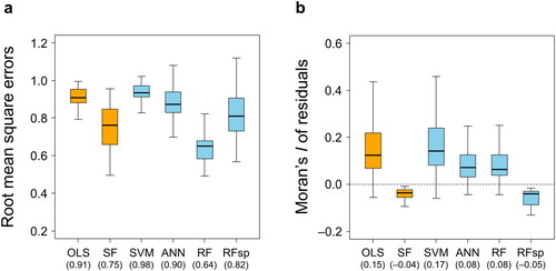
Spatial filtering regression outperformed the other approaches tested with residual Moran’s I values closest to zero (Figure 1(b)). Although the mean Moran’s I of the residuals resulting from RFsp was also close to zero, approximately 23% of these I values (nine out of 39) were lower than −0.1, indicating a potential overcorrection effect for residual autocorrelation by this method (Kim 2021; M. Bini personal communication). There was no significant difference in the mean residual Moran’s I between OLS and SVM (p = 0.971; Supplementary Table S5). In general, these findings were consistent even when the magnitude and SAC of the residuals were analyzed separately for each study site (Supplementary Figures S1 and S2).

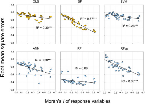
Figure 2. Relationships between spatial autocorrelation (SAC) of each response (soil) variable and RMSE. All SAC is represented by global Moran’s I. Each plot aggregates the findings of all individual study sites (supplementary Figure S3). the orange and sky blue colours indicate non-ML and ML methods, respectively. Linear regression models denoted by *** are significant at the level of p < 0.001. See supplementary Figure S3 for the results obtained by examining variations in the magnitude of the residuals separately for each study site.

3.2. Variation in the magnitude and SAC of the residuals

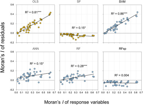
The RMSE values produced by all methods, except RF, had a significantly negative correlation with the Moran’s I of the response variables (Figure 2). This relationship was strongest for the two spatially explicit approaches—SF and RFsp. With the exception of these two methods, the Moran’s I values of the residuals were significantly and positively correlated with the Moran’s I of the response variables (Figure 3). These correlations were also found when variations in the magnitude and SAC of the residuals were examined separately for each study site (Supplementary Figure S3).

Figure 3. Relationships between SAC of each response (soil) variable and SAC of the model residuals. All SAC is represented by global Moran’s I. Each plot aggregates the findings of all individual study sites (supplementary Figure S3). the orange and sky blue colours indicate non-ML and ML methods, respectively. Linear regression models denoted by *** and * are significant at the level of p < 0.001 and p < 0.05, respectively. See supplementary Figure S3 for the results obtained by examining variations in the SAC of the residuals separately for each study site.

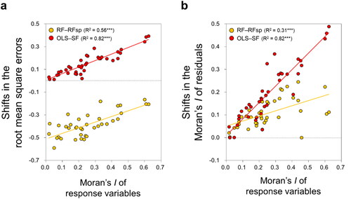
Differences (or shifts) between OLS and SF and between RF and RFsp in both the RMSE and Moran’s I values of the residuals were significantly and positively correlated with the degree of SAC in the response variables (Figure 4). These shifts were calculated as the difference between either OLS and SF (OLS–SF) or RF and RFsp (RF–RFsp); larger shifts indicate greater improvement of model performance by spatially explicit models compared to their non-spatial counterparts.

Figure 4. (a) Relationships between SAC of each response (soil) variable and the reduction in RMSE after incorporating SAC into OLS and RF. (b) Relationships between the SAC of each response variable and the reduction in the SAC of the model residuals after incorporating SAC into OLS and RF. All SAC is represented by global Moran’s I. Each plot aggregates the findings of all individual study sites. Linear regression models denoted by *** are significant at the level of p < 0.001.

3.3. Relative importance of the predictor variables

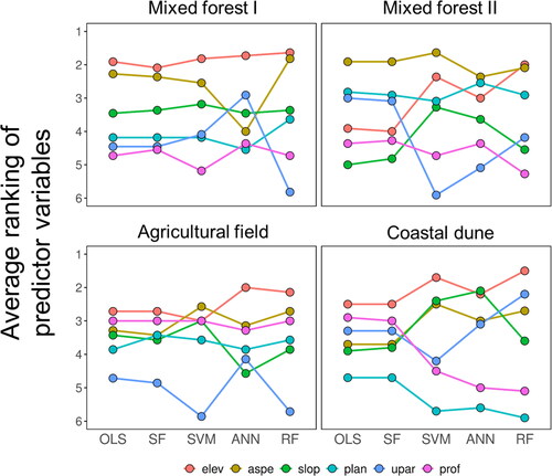
In general, we observed inconsistencies in the relative importance of the predictor variables to soil spatial variability across non-ML and ML approaches or across study sites (Figure 5). That is, no predictor variable was found to have a pervasive pedogeomorphological control on soil properties regardless of modelling methods or landscapes considered. Surface elevation, for example, seemed to be most influential at the mixed forest I site, but its importance decreased at the mixed forest II site, especially when OLS or SF was used. Plan profile was least important in the coastal dune, whereas it was the second or third important predictor at the mixed forest II site. Despite these substantial variabilities, both non-ML algorithms exhibited highly consistent average rankings of the landform attributes within each study site. In other words, the rank orders produced by OLS remained almost always the same as the orders yielded by SF (with the exception of plan curvature in the agricultural field); this consistency was not observed among the ML approaches.

Figure 5. Relative predictive importance of the landform variables in five modelling approaches (RFsp not applicable). at each individual study site, the average ranking of each landform variable was calculated from the multiple soil variables tested (elev, elevation; aspe, slope aspect; slop, slope angle; plan, plan curvature; upar, upslope area; prof, profile curvature).

4. Discussion

4.1. Effects of spatial autocorrelation on modelling results

Our results demonstrate that ML algorithms, although having gained much popularity in various disciplines over the last two decades, when used for the spatial modelling of soil properties, are sensitive to SAC in the input variables. Prediction accuracy has been the central focus and justification of using ML approaches (Wadoux et al. 2020), but three of the four ML methods employed in this study (SVM, ANN, and RFsp) showed larger or similar mean RMSEs compared to the non-ML OLS and SF models (Figure 1(a); Supplementary Figure S1). On average, residuals of the ML models retained more of the SAC inherent in the input variables when compared to SF (Figure 1(b); Supplementary Figure S2). The magnitude and SAC of the residuals were comparatively low for RF and RFsp, respectively; however, despite having the lowest mean RMSE, residual autocorrelation was still present in RF, a finding similar to the description of RF by Georganos et al. (2021). This may be the result of RF-overfitting and/or the SAC inherent in the observations of the training dataset, the latter potentially affecting RF internal cross-validation (Makungwe et al. 2021). Although RFsp reduced the level of residual SAC, the usefulness of this method appeared to be substantially reduced due to the unstable variation (i.e. wide range) of the RMSE values it yielded.

This work confirms that both the magnitude and spatial structure of the residuals resulting from several widely-used ML algorithms in the recent geosciences literature are potentially predictable based on knowledge of the SAC present in the input data. The significant and linear relationships shown in Figures 2 and 3 suggest that the original spatial structure of the soil properties can likely serve as a direct predictor of the autocorrelation that will remain in the residuals after the applications of such ML methods as SVM, ANN, and RF. In addition, the Moran’s I of the soil data can also be used to predict how much improvement (i.e. decreases in RMSE or residual SAC) a non-spatial model, such as OLS and RF, will undergo if the SAC of the response variable is properly accounted for by SF and RFsp, respectively (Figure 4). These findings are consistent with previous research investigating applications of non-ML techniques to spatial modelling of soil properties (Kim et al. 2016, 2019), water quality (Miralha and Kim 2018), species diversity (Kim 2021), and socio-economic phenomena (Kim and Song 2021; Song and Kim in press).

Our findings point to the necessity of taking SAC into account in both non-ML and ML approaches as SAC in the residuals increases linearly with increasing levels of SAC in the response variables. Thus, care should be taken to examine the spatial structure of the response variables when using both non-ML and ML methods. When a soil variable has a low amount of inherent SAC (i.e. Moran’s I < 0.1 in this research), we recommend the use of RF as it yielded the lowest RMSE among the approaches tested in this study (Figure 2) and most of the Moran’s I values of the residuals were very close to zero (Figure 3). If a soil variable is strongly autocorrelated (especially, when Moran’s I > 0.4), however, SF appears to be a better technique because the residual SAC it produces is closer to zero than that of RF with little difference in the RMSE values between the two methods. These findings open the possibility of selecting model types through the establishment of threshold criteria for easily measurable data characteristics, such as, SAC of input variables.

Our results also demonstrate that efforts to identify important factors of soil spatial variability across landscapes can lead to substantially different (even reversed) findings between non-ML and ML approaches (Figure 5). Accordingly, we urge caution that some GIS-based predictor variables, which are considered important in ML models, may prove to be less important in the context of non-ML approaches. Moreover, the above-mentioned RF-overfitting issue suggests that the relative importance of predictor variables may be influenced by the spatially specific mechanism of predictors on each prediction (Shukla et al. 2018; Gupta et al. 2021). These discussions become all the more important when these models are directly used to understand possible physical and chemical processes that shape the patterns of soil–landform couplings in a system of interest.

4.2. Limitations and future opportunities

Each ML approach presents inherent limitations when it comes to both the reduction of residual SAC and the attainment of predictive accuracy. SVM employs regularization to prevent overfitting, which can yield lower predictive accuracy in small datasets. Also, a higher level of residual SAC from SVM results is possibly due to relatively lower degree of nonlinearity of SVM compared to that of other ML techniques. Moreover, the decision-making around kernel selection complicates the SVM's model selection process, making it more challenging than that of the other tested ML models. We demonstrated that ANN reduce residual SAC when compared to SVM and RF, despite its predictive accuracy remaining on par with that of SVM; however, these results may stem from the small datasets used in this study to train the ANN. RF showed lower RMSEs than the other ML methods due to randomization of predictor selection and resampling. Additionally, residual SAC was directly proportional to SAC in the response variables, potentially offsetting the enhanced predictive performance of RF when dealing with highly spatially autocorrelated response variables. Despite the efficacy of RFsp in mitigating residual SAC compared to conventional RF, it introduces increased computational complexity through the addition of a distance matrix (N by N where N is the number of observations) into the input data matrix. The unique nature of this distance matrix within RFsp makes the comparison of predictive accuracy difficult using the conventional train-test split procedures, since the distance matrix is unique to each set of input data. The limitations of each ML approach require careful consideration. The objective of the soil–geomorphic modelling—whether to reduce residual SAC or enhance predictive accuracy of soil properties—should guide the selection of the most appropriate model.

Although some of the differences in residual SAC presented in this paper are attributable to the use of insufficient predictor data (e.g. the use of only six landform variables extracted by GIS-based terrain analysis), high spatial density of the samples (Supplementary Information II), or the complexity and uncertainty of the data associated with non-stationarity (Kim 2021), our findings suggest that further work is needed to understand the comparative usefulness of ML approaches over conventional non-ML methods. Future studies can improve the issue of limited predictor variables using, for example, multi-hierarchical relief attributes especially when scale-specific dependencies exist between the representativeness of the soil samples and the explanatory power of the variables used (Behrens et al. 2018c; Guo et al. 2019; Möller et al. 2022). In addition, when multi-collinearity is expected to impair model interpretability and lead to misidentification of relevant predictors (Dormann et al. 2013; cf. Supplementary Table S6), future soil–landform modelers are recommended to test VI employing downstream examinations like the recursive feature elimination approach (Guyon et al. 2002; Svetnik et al. 2004).

5. Conclusions

Spatial autocorrelation exists nearly ubiquitously in soil–geomorphic data, and can provide useful information that researchers can include into the modelling of natural resources. Our findings demonstrate that this inherent spatial structure in soil–geomorphic data often significantly affects the outcomes of common ML algorithms in terms of the magnitude and autocorrelation of the residuals and the predictive importance of landform variables to soil spatial variability. We conclude that the level of SAC in the input variables can be used to guide the selection of appropriate non-ML or ML approaches making model choices more consistent across divergent pedogeomorphological systems.

Acknowledgements

The original version of this paper was substantially improved thanks to the constructive comments by three anonymous reviewers.

Data availability statement

Codes and datasets used in this study can be found in the online repository: https://github.com/biogeokim/ml_soil_sac_prediction.

Disclosure statement

The authors declare that they have no known competing financial interests or personal relationships that could have affected the work presented in this paper.

Correction Statement

This article has been corrected with minor changes. These changes do not impact the academic content of the article.

Additional information

Funding

This research was supported by the National Science Foundation (No. 1560907) and the National Research Foundation of Korea grant funded by the Korea government (No. 2021R1I1A2047661). Participation of PŠ was covered by the Technology Agency of the Czech Republic project No. SS02030018.

References

- Abu-Mostafa YS, Magdon-Ismail M, Lin HT. 2012. Learning from data. United States: AMLBook.
- Angelini ME, Heuvelink GBM. 2018. Including spatial correlation in structural equation modelling of soil properties. Spatial Stat. 25:35–51. doi: 10.1016/j.spasta.2018.04.003.
- Anselin L. 2002. Under the hood: issues in the specification and interpretation of spatial regression models. Agric Econ. 27(3):247–267. doi: 10.1111/j.1574-0862.2002.tb00120.x.
- Behrens T, Schmidt K, MacMillan RA, Rossel RAV. 2018a. Multi-scale digital soil mapping with deep learning. Sci Rep. 8(1):15244. doi: 10.1038/s41598-018-33516-6.
- Behrens T, Schmidt K, Viscarra Rossel RA, Gries P, Scholten T, MacMillan R. 2018b. Spatial modelling with Euclidean distance fields and machine learning. Eur J Soil Sci. 69(5):757–770. doi: 10.1111/ejss.12687.
- Behrens T, Schmidt K, MacMillan RA, Rossel RAV. 2018c. Multiscale contextual spatial modelling with the Gaussian scale space. Geoderma. 310:128–137. doi: 10.1016/j.geoderma.2017.09.015.
- Bel L, Laurent JM, Bar-Hen A, Allard D, Cheddadi R. 2005. A spatial extension of CART: application to classification of ecological data. In: Renard P, Demougeot-Renard H, Froidevaux R, editors. Geostatistics for environmental applications. Berlin: Springer; p. 99–109.
- Bischl B, Lang M, Kotthoff L, Schiffner J, Richter J, Studerus E, Casalicchio G, Jones ZM. 2016. Mlr: Machine learning in R. J Mach Learn Res. 17:1–5.
- Bivand RS, Pebesma E, Gómez-Rubio V. 2013. Applied spatial data analysis with R. New York, NY: Springer.
- Breiman L. 2001. Random forests. Mach Learn. 45(1):5–32. doi: 10.1023/A:1010933404324.
- Brungard CW, Boettinger JL, Duniway MC, Wills SA, Edwards TC. 2015. Machine learning for predicting soil classes in three arid landscapes. Geoderma. 239–240:68–83. doi: 10.1016/j.geoderma.2014.09.019.
- Burrough PA. 2001. GIS and geostatistics: essential partners for spatial analysis. Environ Ecol Stat. 8(4):361–377. doi: 10.1023/A:1012734519752.
- Chang CC, Lin CJ. 2011. LIBSVM: a library for support vector machines. ACM Trans Intell Syst Technol. 2(3):1–27. doi: 10.1145/1961189.1961199.
- Currit N. 2002. Inductive regression: overcoming OLS limitations with the general regression neural network. Comput Environ Urban Syst. 26(4):335–353. doi: 10.1016/S0198-9715(01)00045-X.
- Dormann CF, Elith J, Bacher S, Buchmann C, Carl G, Carré G, Marquéz JRG, Gruber B, Lafourcade B, Leitão PJ, et al. 2013. Collinearity: a review of methods to deal with it and a simulation study evaluating their performance. Ecography. 36(1):27–46. doi: 10.1111/j.1600-0587.2012.07348.x.
- Drucker H, Surges CJC, Kaufman L, Smola A, Vapnik V. 1997. Support vector regression machines. Adv Neural Inf Process Syst. 1:155–161.
- Ferraciolli MA, Bocca FF, Rodrigues LHA. 2019. Neglecting spatial autocorrelation causes underestimation of the error of sugarcane yield models. Comput Electron Agric. 161:233–240. doi: 10.1016/j.compag.2018.09.003.
- Feurer M, Hutter F. 2019. Hyperparameter optimization. In: Hutter F, Kotthoff L, Vanschoren J, editors. Automated machine learning: methods, systems, challenges. The Springer series on challenges in machine learning. Cham: Springer International Publishing; p. 3–33. doi: 10.1007/978-3-030-05318-5_1.
- Fisher A, Rudin C, Dominici F. 2019. All models are wrong, but many are useful: learning a variable’s importance by studying an entire class of prediction models simultaneously. J Mach Learn Res. 20:1–81.
- Gaspard G, Kim D, Chun Y. 2019. Residual spatial autocorrelation in macroecological and biogeographical modeling: a review. J Ecol Environ. 43:19. doi: 10.1186/s41610-019-0118-3.
- Georganos S, Grippa T, Niang Gadiaga A, Linard C, Lennert M, Vanhuysse S, Mboga N, Wolff E, Kalogirou S. 2021. Geographical random forests: a spatial extension of the random forest algorithm to address spatial heterogeneity in remote sensing and population modelling. Geocarto Int. 36(2):121–136. doi: 10.1080/10106049.2019.1595177.
- Getis A, Griffith DA. 2002. Comparative spatial filtering in regression analysis. Geogr Anal. 34(2):130–140. doi: 10.1111/j.1538-4632.2002.tb01080.x.
- Grekousis G. 2019. Artificial neural networks and deep learning in urban geography: a systematic review and meta-analysis. Comput Environ Urban Syst. 74:244–256. doi: 10.1016/j.compenvurbsys.2018.10.008.
- Griffith DA. 2000. A linear regression solution to the spatial autocorrelation problem. J Geograph Syst. 2(2):141–156. doi: 10.1007/PL00011451.
- Griffith DA. 1996. Spatial autocorrelation and eigenfunctions of the geographic weights matrix accompanying geo-referenced data. Canadian Geographer. 40(4):351–367. doi: 10.1111/j.1541-0064.1996.tb00462.x.
- Griffith DA. 2003. Spatial autocorrelation and spatial filtering: gaining understanding through theory and scientific visualization. Berlin: Springer-Verlag.
- Grömping U. 2009. Variable importance assessment in regression: linear regression versus random forest. Am Stat. 63(4):308–319. doi: 10.1198/tast.2009.08199.
- Guo Z, Adhikari K, Chellasamy M, Greve MB, Owens PR, Greve MH. 2019. Selection of terrain attributes and its scale dependency on soil organic carbon prediction. Geoderma. 340:303–312. doi: 10.1016/j.geoderma.2019.01.023.
- Gupta S, Lehmann P, Bonetti S, Papritz A, Or D. 2021. Global prediction of soil saturated hydraulic conductivity using random forest in a covariate-based geotransfer function (CoGTF) framework. J Adv Model Earth Syst. 13(4):e2020MS002242. doi: 10.1029/2020MS00224.
- Guyon I, Weston J, Barnhill S, Vapnik V. 2002. Gene selection for cancer classification using support vector machines. Mach Learn. 46(1/3):389–422. doi: 10.1023/A:1012487302797.
- Head ML, Holman L, Lanfear R, Kahn AT, Jennions MD. 2015. The extent and consequences of p-hacking in science. PLoS Biol. 13(3):e1002106. doi: 10.1371/journal.pbio.1002106.
- Hengl T, Nussbaum M, Wright MN, Heuvelink GBM, Gräler B. 2018. Random forest as a generic framework for predictive modeling of spatial and spatio-temporal variables. PeerJ. 6:e5518. doi: 10.7717/peerj.5518.
- Heung B, Ho HC, Zhang J, Knudby A, Bulmer CE, Schmidt MG. 2016. An overview and comparison of machine-learning techniques for classification purposes in digital soil mapping. Geoderma. 265:62–77. doi: 10.1016/j.geoderma.2015.11.014.
- Heuvelink GBM, Webster R. 2022. Spatial statistics and soil mapping: a blossoming partnership under pressure. Spatial Stat. 50:100639. doi: 10.1016/j.spasta.2022.100639.
- Jiang Z, Li Y, Shekhar S, Rampi L, Knight J. 2017. Spatial ensemble learning for heterogeneous geographic data with class ambiguity: a summary of results. Proceedings of the 25th ACM SIGSPATIAL International Conference on Advances in Geographic Information Systems 23. p. 1–10. doi: 10.1145/3139958.3140044.
- Kanevski M, Timonin V, Pozdnukhov A. 2009. Machine learning for spatial environmental data: theory, applications, and software. Boca Raton: CRC Press LLC.
- Kaya F, Mishra G, Francaviglia R, Keshavarzi A. 2023. Combining digital covariates and machine learning models to predict the spatial variation of soil cation exchange capacity. Land. 12(4):819. doi: 10.3390/land12040819.
- Khaledian Y, Miller BA. 2020. Selecting appropriate machine learning methods for digital soil mapping. Appl Math Modell. 81:401–418. doi: 10.1016/j.apm.2019.12.016.
- Kim D. 2021. Predicting the magnitude of residual spatial autocorrelation in geographical ecology. Ecography. 44(7):1121–1130. doi: 10.1111/ecog.05403.
- Kim D, Song I. 2021. Predicting model improvement by accounting for spatial autocorrelation: a socio-economic perspective. Prof Geogr. 73(1):131–149. doi: 10.1080/00330124.2020.1812408.
- Kim D, Hirmas DR, McEwan RW, Mueller TG, Park SJ, Šamonil P, Thompson JA, Wendroth O. 2016. Predicting the influence of multi-scale spatial autocorrelation on soil–landform modeling. Soil Sci Soc Am J. 80(2):409–419. doi: 10.2136/sssaj2015.10.0370.
- Kim D, Šamonil P, Jeong G, Tejnecký V, Drábek O, Hruška J, Park SJ. 2019. Incorporation of spatial autocorrelation improves soil–landform modeling at A and B horizons. Catena. 183:104226. doi: 10.1016/j.catena.2019.104226.
- Kühn I, Dormann CF. 2012. Less than eight (and a half) misconceptions of spatial analysis. J Biogeogr. 39(5):995–998. doi: 10.1111/j.1365-2699.2012.02707.x.
- Kuhn M, Johnson K. 2013. Applied predictive modeling. New York, NY: Springer.
- Lark RM. 2012. Towards soil geostatistics. Spatial Stat. 1:92–99. doi: 10.1016/j.spasta.2012.02.001.
- Legendre P. 1993. Spatial autocorrelation: trouble or new paradigm? Ecology. 74(6):1659–1673. doi: 10.2307/1939924.
- Makungwe M, Chabala LM, Chishala BH, Lark RM. 2021. Performance of linear mixed models and random forests for spatial prediction of soil pH. Geoderma. 397:115079. doi: 10.1016/j.geoderma.2021.115079.
- Ma Y, Minasny B, Malone BP, McBratney AB. 2019. Pedology and digital soil mapping (DSM). Eur J Soil Sci. 70(2):216–235. doi: 10.1111/ejss.12790.
- McBratney AB, Santos MLM, Minasny B. 2003. On digital soil mapping. Geoderma. 117(1–2):3–52. doi: 10.1016/S0016-7061(03)00223-4.
- Miralha L, Kim D. 2018. Accounting for and predicting the influence of spatial autocorrelation in water quality modeling. IJGI. 7(2):64. doi: 10.3390/ijgi7020064.
- Molnar C. 2022. Interpretable machine learning. Lulu. com. Victoria, BC: Leanpub.
- Möller M, Zepp S, Wiesmeier M, Gerighausen H, Heiden U. 2022. Scale-specific prediction of topsoil organic carbon contents using terrain attributes and SCMaP soil reflectance composites. Remote Sens. 14(10):2295. doi: 10.3390/rs14102295.
- Montgomery DC, Peck EA, Vining GG. 2012. Introduction to linear regression analysis. Hoboken, NJ: Wiley.
- Nussbaum M, Spiess K, Baltensweiler A, Grob U, Keller A, Greiner L, Schaepman ME, Papritz A. 2018. Evaluation of digital soil mapping approaches with large sets of environmental covariates. Soil. 4(1):1–22. doi: 10.5194/soil-4-1-2018.
- Nikparvar B, Thill JC. 2021. Machine learning of spatial data. IJGI. 10(9):600. doi: 10.3390/ijgi10090600.
- O’Callaghan JF, Mark DM. 1984. The extraction of drainage networks from digital elevation data. Comput Vision Graphics Image Process. 28(3):323–344. doi: 10.1016/S0734-189X(84)80011-0.
- R Core Team. 2021. R: the R Project for statistical computing.
- Schölkopf B, Smola AJ, Williamson RC, Bartlett PL. 2000. New support vector algorithms. Neural Comput. 12(5):1207–1245. doi: 10.1162/089976600300015565.
- Schölkopf B, Smola AJ. 2001. Learning with kernels: support vector machines, regularization, optimization, and beyond. Cambridge, MA: MIT Press.
- Schratz P, Muenchow J, Iturritxa E, Richter J, Brenning A. 2019. Performance evaluation and hyperparameter tuning of statistical and machine-learning models using spatial data. Ecol Modell. 406:109–120. doi: 10.1016/j.ecolmodel.2019.06.002.
- Sekulić A, Kilibarda M, Heuvelink GBM, Nikolić M, Bajat B. 2020. Random forest spatial interpolation. Remote Sens. 12(10):1687. doi: 10.3390/rs12101687.
- Sergeev AP, Buevich AG, Baglaeva EM, Shichkin AV. 2019. Combining spatial autocorrelation with machine learning increases prediction accuracy of soil heavy metals. Catena. 174:425–435. doi: 10.1016/j.catena.2018.11.037.
- Shukla G, Garg RD, Srivastava HS, Garg PK. 2018. An effective implementation and assessment of a random forest classifier as a soil spatial predictive model. Int J Remote Sens. 39(8):2637–2669. doi: 10.1080/01431161.2018.1430399.
- Sinha P, Gaughan AE, Stevens FR, Nieves JJ, Sorichetta A, Tatem AJ. 2019. Assessing the spatial sensitivity of a random forest model: application in gridded population modeling. Comput Environ Urban Syst. 75:132–145. doi: 10.1016/j.compenvurbsys.2019.01.006.
- Svetnik V, Liaw A, Tong C, Wang T. 2004. Application of Breiman’s random forest to modeling structure-activity relationships of pharmaceutical molecules [series title: lecture notes in computer science]. In: T Kanade, J Kittler, JM Kleinberg, F Mattern, JC Mitchell, M Naor, O Nierstrasz, C Pandu Rangan, B Steffen, M Sudan, D Terzopoulos, D Tygar, MY Vardi, G Weikum, F Roli, J Kittler, T Windeatt, editors, Multiple classifier systems. Berlin Heidelberg: Springer; p. 334–343. doi: 10.1007/978-3-540-25966-4_33.
- Tiefelsdorf M, Griffith DA. 2007. Semiparametric filtering of spatial autocorrelation: the eigenvector approach. Environ Plan A. 39(5):1193–1221. doi: 10.1068/a37378.
- van der Westhuizen S, Heuvelink GBM, Hofmeyr DP, Poggio L. 2022. Measurement error-filtered machine learning in digital soil mapping. Spatial Stat. 47:100572. doi: 10.1016/j.spasta.2021.100572.
- Venables WN, Ripley BD. 2002. Modern applied statistics with S. New York, NY: Springer.
- Wadoux AMJC. 2019. Using deep learning for multivariate mapping of soil with quantified uncertainty. Geoderma. 351:59–70. doi: 10.1016/j.geoderma.2019.05.012.
- Wadoux AMJC, Minasny B, McBratney AB. 2020. Machine learning for digital soil mapping: applications, challenges and suggested solutions. Earth-Sci Rev. 210:103359. doi: 10.1016/j.earscirev.2020.103359.
- Wadoux AMJC, Padarian J, Minasny B. 2019. Multi-source data integration for soil mapping using deep learning. Soil. 5(1):107–119. doi: 10.5194/soil-5-107-2019.
- Wright MN, Ziegler A. 2017. ranger: a fast implementation of random forests for high dimensional data in C++ and R. J Stat Soft. 77(1):17. doi: 10.18637/jss.v077.i01.
- Zevenbergen LW, Thorne CR. 1987. Quantitative analysis of land surface topography. Earth Surf Process Landforms. 12(1):47–56. doi: 10.1002/esp.3290120107.