Analysis of future meteorological, hydrological, and agricultural drought characterization under climate change in Kessie watershed, Ethiopia

Abstract

The objective of this study is to analyze future drought characteristics in meteorological, hydrology, and agricultural droughts under the impact of changing climate in the Kessie watershed, upper Blue Nile Basin, using three drought indices; Reconnaissance Drought Index (RDI), Streamflow Drought Index (SDI) and Agricultural Standardized Precipitation Index (aSPI), respectively. The study used baseline data (1985–2014) and future (2041–2100) downscaled from Coupled Model Intercomparison Project 6 (CMIP-6) based on the three Global Climate Models (GCMs) projections under two scenarios of the Shared Socioeconomic Pathways (SSP) (SSP2-4.5, SSP5-8.5) with well-calibrated Soil and Water Assessment Tool (SWAT) model to simulate future streamflow for two future time horizons 2050s (2041–2070) and 2080s (2071–2100). Based on the yearly time scale, our results indicate that droughts of a high magnitude and rising frequency would affect most of the research area. These droughts will be either meteorological (RDI), agricultural (aSPI), or hydrological (SDI). Short-term agricultural and hydrological droughts are also anticipated to occur more frequently. The projected increases in frequency and trend of agricultural and hydrological droughts in this area are greater due to the anticipated drop in annual rainfall and the larger increase in mean annual temperature in the middle of Kessie. Furthermore, compared to hydrological and agricultural droughts, meteorological drought is less vulnerable to climate change; but, as the accumulation period lengthens, a stronger association develops between hydrological and agricultural droughts. These findings may be useful for water resources management and future planning for mitigation and adaptation to the climate change impact in the study area.

Keywords:

• Climate change
• CMIP6
• drought indices
• SWAT
• Kessie watershed

1. Introduction

Water availability is limited in a particular natural and/or social system during a drought. It is a significant category of natural disaster and one of the most significant consequences of climate change on ecosystems and people (Sheffield et al. 2012; Zeng et al. 2022). Drought can be harmful to the environment, economy, agriculture, energy, and human health (Ahmadalipour and Moradkhani 2018). Drought is thought to be responsible for a third of all economic consequences from natural disasters, with annual losses to the global economy estimated to reach over 6 billion US dollars (AghaKouchak et al. 2015). According to many climate change predictions, droughts and dry spells are predicted to alter in various places, bringing hazards to both natural and social systems (Cook et al. 2018; Hessl et al. 2018; Seager et al. 2019; Asadi Zarch 2022).

Although the scientific community has not agreed on a single definition of drought, four distinct forms of drought—meteorological (related to a lack of precipitation), hydrological (related to a shortage of surface and sub-surface water), agricultural (related to a lack of soil moisture), and socioeconomic (related to an imbalance between supply and demand) that can occur in various but interconnected systems have been identified in earlier studies (Wilhite and Glantz 1985; Tallaksen and Van Lanen 2004; Lloyd-Hughes 2014). A single index may not be adequate for a detailed characterization of drought, according to studies, hence a multi-index approach should be taken into account (Cook et al. 2020; Wang et al. 2021). Typically, the initial step of a compound drought occurrence is meteorological drought, which serves as the catalyst or initiating factor for hydrological and/or agricultural drought (Yuan et al. 2017).

Due to their reliance on rain-fed agriculture, the majority of African nations are particularly exposed to the threats of climate change, including floods and droughts (Kusangaya et al. 2014; Gemeda and Sima 2015). For example, predictions indicate that the October–December 2022 rainy season would underperform, making it the fifth consecutive failed season in regions of Ethiopia, Kenya, and Somalia, where droughts are presently posing an immediate threat of starvation (Levy et al. 2022). Due to inconsistent rainfall and climate change, Ethiopia has experienced seasonal droughts frequently for a long time (Philip et al. 2018). Several Amhara provinces, including South Wollo, North Wollo, South Gondar, and Afar, as well as the entirety of Somalia Region, Eastern portions of Oromia Region, and the Upper Blue Nile basin in northeastern Ethiopia, which includes the Northern Tigray region, are particularly vulnerable to drought in Ethiopia (Loakes 2016; Bayissa et al. 2018; Melaku 2020). it is important in practice to analyze the characteristics of precipitation and temperature in the upper Blue Nile River Basin under future scenarios.

However, the drought index is a useful technical tool for quantitatively assessing and characterizing drought episodes (Yihdego et al. 2019). The commonly used indicators for meteorological drought index are the Standardized Precipitation Index (SPI) (Livada and Assimakopoulos 2007; Waseem et al. 2022) Standardized Precipitation evaporation Index (SPEI) (Beguería et al. 2014; Liu et al. 2021) and Reconnaissance Drought Index (RDI) (Tsakiris et al. 2007), hydrological drought (Streamflow Drought Index: SDI) (Nazarenko et al. 2023) and Agricultural Drought (Agricultural Standardized Precipitation Index: aSPI) (Tigkas et al. 2022). Drought is still not well studied in Ethiopia both at the national and basin level. Relatively, meteorological drought analysis is studied in different basins of the country due to the easy accessibility of observed and satellite-recorded precipitation data. To balance the potential water supply and demand, further research on the hydrological and agricultural drought is still required.

In the Upper Blue Nile basin, previous researchers have made an effort to use satellite data to analyze the frequency and severity of meteorological droughts. For example, according to research on the spatial-temporal assessments of SPI values in the upper Blue Nile basin, (Bayissa et al. 2015) found that seasonal or yearly meteorological drought spells occurred in the years 1978/79, 1984/85, 1994/95, and 2003/04 and According to Taye et al. (2020) over the course of the 38-year period, the frequency of severe/extreme meteorological drought varied from 7% to 11% across the highland, midland, and lowland sections of the Upper Blue Nile basin. Both authors use historical data on the basin to analyze drought, although only one of the sub-basins of the Upper Blue Nile basin (Abbay), Kessie Watershed, is sensitive to agroclimatic zone and drought analysis (Enyew et al. 2014; Taye 2021). Analysis of the impending hydrological, meteorological and Agricultural droughts in the Kessie watershed of the Upper Blue Nile basin is therefore essential.

Unlike the typical concentration pathways (RCPs) scenarios in CMIP5, the scenarios in CMIP6 are combined scenarios of different shared socioeconomic pathways (SSPs) and RCPs, which contain implications for future socio-economic development (Fujimori et al. 2017). The most recent version of scenarios, known as Shared Socio-Economic Pathways (SSPs), was used for Coupled Model Intercomparison Project 6 (CMIP-6) and the IPCC Sixth Assessment Report (IPCC 2021).

The goal of this study was to examine the effects of climate change on meteorological, hydrological, and agricultural droughts in the Kessie watershed in the upper Blue Nile Basin using two combining SSP2 (SSP2-4.5), and SSP5 (SSP5-8.5) released by CMIP-6 climate model projections for historical periods (1985–2014), and future periods (2041–2099). The findings of this study should provide water managers with deeper understanding of how droughts in the study area are impacted by climate change.

2. Methodology

2.1. Study area description

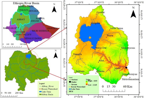
The upper Blue Nile is the largest contributor to the Nile River’s, which accounts for more than 60% of the total flow (Conway 2000). The Kessie watershed (case study watershed) is part of the upper Blue Nile basin (shown Figure 1). It is located in the northern part of the upper Blue Nile Basin and the area coverage is about 23,580 km². The geographic location of the case-study watershed is between 10° 40′ to 12° 45′ N and 36° 40′ to 38° 15′E. The elevation of the study area is from 1249 to 4103 meters above mean sea level (Figure 1).

Figure 1. Locations of the study area with elevation and metrological stations.

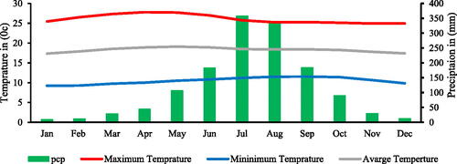
The Kessie watershed has higher rainfall in July and August and lower rainfall from December to February. The watershed receives intermediate rainfall, lower rainfall than in July and August but higher rainfall than the remaining months, in June and September. From the total annual rainfall, 70% to 90% occurs from June to September. The range of average annual precipitation in the watershed was found to be 1049 mm to 2310 mm per year. The mean daily minimum and maximum temperatures of the catchment are 6.78 °C and 29.86 °C, respectively, according to the thirty years (1985–2014) of temperature data and average monthly distribution show in Figure 2.

Figure 2. Long term average monthly precipitation and temperature (1985–2014).

2.1.1. Observed hydro-meteorological data

The observed meteorological data used for this study were temperatures (both minimum and maximum), rainfall, wind speed, wind direction, relative humidity, sunshine hours, and solar radiation. These data (1985–2014) were collected from the Ethiopian National Meteorological Agency (NMA), Addis Ababa, and Bahir Dar Branch. The details of the data were used this study indicated in Tables 1 and 2. The weather generator, which is used to provide data for stations with missing data, was prepared manually by using PCPSTAT and dewPOINT2.0 version programs on 30-year rainfall, temperature, and wind data. PCPSTAT is program or tool used to prepared precipitation Data for SWAT input (website: http://www.brc.tamus.edu/swat/pcpSTAT.zip). With the help of this program, statistical parameters for SWAT's average daily precipitation data were calculated in the < userwgn.dbf>. The beginning and last values in the precipitation input file must be used for January 1 and December 31, respectively. The program dewPOINT2.0 was used to calculate average daily dewpoint temperature per month. This application used daily maximum and minimum temperature and mean humidity data to get the average daily dew point temperatures. similar to PCPSTAT, the dewPOINT2.0 was done by initial and end values in the input file from January 1 and December 31, respectively. The dewPOINT2.0 was calculated as follows: (1) $$\mathit{dew}=\left(234.18\mathrm{\hspace{0.17em}*\hspace{0.17em}}\log 10\right(ea)-184.2)/\left(8.204\text{-}\log 10\right(ea\left)\right)\mathrm{ }$$(1) (2) $$ea=RF\mathrm{\hspace{0.17em}*\hspace{0.17em}}\frac{es}{100}$$(2) (3) $$es=0.6108\mathrm{\hspace{0.17em}*\hspace{0.17em}}\exp \hspace{0.17em}(\left(17.27\mathrm{\hspace{0.17em}*\hspace{0.17em}}T\right)/(T+\mathrm{ }237.3))$$(3) where, es is saturation vapour pressure [hPa], ea is actual vapour pressure [hPa], exp is 2.7183 (base of natural logarithm), T is air temperature [^oC], RF is relative humidity [%] and dew is dewpoint temperature [^oC].

Table 1. Data type, sources and purpose.

Data type	Source	Purpose
Meteorological data	Ethiopia meteorological agency (Addis Ababa and Bahir-Dar Branch)	Input for SWAT model to simulate the streamflow, and used as a reference for trend analysis
Hydrological data	Ministry of Energy and Water Recourse, Ethiopia	SWAT model Simulation calibration and Validation
DEM (20 m*20m)	USGS (http://earthexplorer.usgs.gov/)	SWAT watershed Delineation, and to develop slope and elevation.
Soil (1: 250,000)	Ministry of Water and Energy	SWAT - HRU definition and to prepare the soil map of the study area
Land use (1: 250,000)	Ministry of Water and Energy	SWAT - HRU definition and to prepare the land use map of the study area

Table 2. Metrological and hydrological data availability.

Stations Name	Latitude	Longitude	Altitude	Rainfall	Temperature		Data availability
					Max	min
Adiss zemn	12.11	37.77	1940	✓	✓	✓	1985–2014
Werta	11.92	37.69	1819	✓	✓	✓	1985–2014
Gondar	12.52	37.43	1973	✓	✓	✓	1985–2014
Gorgora	12.24	37.29	1816	✓	–	–	1985–2014
Mekneyesus	11.60	38.05	2374	✓	✓	✓	1985–2014
Deber Tabor	10.32	37.73	2612	✓	✓	✓	1985–2014
Adet	11.27	37.49	2179	✓	✓	✓	1985–2014
Bahir Dar	11.60	37.41	1770	✓	✓	✓	1985–2014
Motta	11.07	37.89	2417	✓	✓	✓	1985–2014
Metrolemariam	10.88	38.28	2676	✓	–	–	1985–2014
Gundweuyne	10.92	38.08903	2052	✓	–	–	1985–2014
Dangila	11.43	36.846	2116	✓	✓	✓	1985–2014
Injibara	10.99	36.9193	2568	✓	–	–	1985–2014
Quarite	10.99	37.431	2147	✓	–	–	1985–2014
Hydrological Data (Gauged location)	Latitude (degree)	Longitude (degree)	Daily Max Discharge (m^3/sec)	Daily Min Discharge (m^3/sec)	Data availability		Recorded length
Abbay at Kessie	11.44 N	38.11 E	7,000	180	1985–2014		30

General Circulation Models (GCMs) are mathematical models that simulate the Earth’s climate system. They use complex algorithms to simulate the interactions between the atmosphere, oceans, land surface, and ice. GCMs are used to make predictions about future climate change and to understand past climate variations. Observed data, on the other hand, refers to actual measurements of climate variables such as temperature, precipitation, and atmospheric composition. These measurements can be taken from various sources such as weather stations. GCMs typically have a coarse spatial resolution, meaning that they cannot capture small-scale features such as local weather patterns or individual storms. Observed data, on the other hand, can provide much higher spatial resolution, allowing for more detailed analysis of local climate variations. Similarly, GCMs operate on a longer time scale than observed data. GCMs simulate climate over decades or centuries, while observed data provides information on shorter time scales such as daily or monthly variations with a point measurement of whether stations. Despite these differences, GCMs and observed data are both important tools for understanding and predicting climate change. GCMs can provide insights into long-term trends and global patterns, while observed data can help validate and improve the accuracy of these models (Table 2).

2.1.2. Spatial data

The spatial data used for this study include the digital elevation model (DEM) (20 m*20m) were downloaded at http://earthexplorer.usgs.gov/, land use and land cover data (1: 250,000) obtained from the Ministry of Water and Energy, and soil type data (1: 250,0000) obtained from Ministry of Water and Energy. The meteorological and spatial data mentioned were used as input to the SWAT model to simulate the streamflow of the case-study watershed. The hydrological (discharge) data was collected at the Ministry of Water and Energy and used for the SWAT model calibration and validation. In addition, DEM data was used to develop the elevation and slope of the study area and the soil data were used to develop the soil map of the study area. The land use data was used to develop the land cover map of the study area. The materials and tools used for the study were ArcGIS10.4, ArcSWAT10.4, XLSTATA2014, Google Earth Pro., SWAT-weather databasev01803, Minitab 18, and SWAT-CUP.

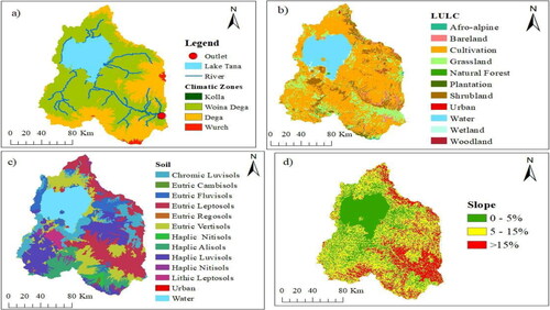
According to Figure 3, the primary land use land cover types are afro-alpine, bare land, cultivation, grassland, forest land, shrub land, urban areas, and water bodies (Figure 3b). Cultivation land (59.25%) is the most common type of land use. The largest lake in Ethiopia, Lake Tana, is included in the case study watershed, which results in a sizable water body (12.97%). Twelve different soil categories, including Chromic Luvisols, Eutric Cambisols, Eutric Fluvisols, Eutric Leptosols, Eutric Vertisols, Haplic Acrisols, Haplic Alisols, Haplic Luvisols, Haplic Nitisols, Haplic Alisols, and Lithic Leptosol, are present in the case study watershed (Figure 3c). Eutric Leptosols (22.14%) and Eutric Vertisols (15.49%) are the two most prevalent soil types in the case-study area. The dominating slope in the case study watershed is 5%, which accounts for around 64.59% of the entire area. This watershed also has a different slope (Figure 3d). About 24.75% of the slope between 5% and 15% and about 10.66% of the slope over 15% are counted. The case study watershed contains four climate groups, namely Kola, Woyna Dega, and Wurch, according to the traditional classification of climate based mostly on altitude variation (Figure 3a). 35% Dega, 31% Weyna-Dega, 25% Kola, and 9% Wurch are all included. Kola is unique to the Lake Tana watershed and its surrounding locations. Kola climatic conditions are also present in the vicinity of the upper Blue Nile River.

Figure 3. (a) Climate classification, (b) land use types, (c) soil types, and (d) slope data.

2.1.3. Global climate model (GCM) data

The Global climate model data outputs with two representative shared socio-economic pathways (SSPs) (SSPs2-4.5 and SSPs5-8.5) were downloaded from CMIP-6 data (Table 3) set website at https://esgf-node.llnl.gov/projects/cmip6/. These data were, after the best-fit climate model outputs to the observed data have been selected, used for the trend analysis of future temperature and precipitation change and used as input for the SWAT model to simulate the future streamflow data.

Table 3. The GCMs data outputs.

GCM Name	Developed by	Resolution	GCM Name	Developed by	Resolution
ACCESS-ESM1-5	Australia	1.87^o × 1.25^o	MPI-ESM1-2-LR	Germany	1.861˚ × 1.875^o
BCC-CSM2-MR	China	1.1^o × 1.1^o	MRI-ESM2-0	Japan	1.1^o × 1.1^o
EC-Earth3	–	–	IITM-ESM	–	–
GFDL-ESM4	USA	1.00^o × 1.25^o	FGOALS-g3	China	2^o× 2.3^o
INM-CM5-0	Russia	2.00^o × 1.50^o	NESM3	China	1.9^o × 1.9^o
MIROC6	Japan	1.4^o × 1.4^o	HadGEM3-GC31-LL	UK	1.25˚ × 1.875˚

2.2. Methods

2.2.1. Observed data quality testing

Performing the data quality test is necessary to provide accurate and precise data to the model and to get a reasonable simulated result. Hydrological studies are usually started with data quality assessments such as checking for outliers, missing data, homogeneity and consistency tests, etc. On hydro-meteorological data, missing data were filled in, a homogeneity and consistency test were performed, and a trend analysis was carried out. For the rainfall and temperature data, missing data were filled by selecting the best method by investigating and comparing their minimum standard error. The absence of a trend test was carried out using the Mann-Kendall trend test using XLSTAT2014 integrated with Excel.

2.2.2. GCMs data bias correction

When downscaling climate data from Global Climate Models (GCMs), there are several variables to consider. These variables help to translate the coarse-resolution GCM output to a finer resolution that better represents the local or regional climate conditions. The variables to include in downscaling climate data from GCMs may vary depending on the specific research or application. However, in this research temperature (minimum and maximum temperature) and precipitation variables were considered.

Bias correction methods are used to adjust GCMs’ output to match observed data. These methods are necessary because GCMs often have biases, or systematic errors, due to limitations in their modeling of physical processes and the coarse spatial resolution of their grid cells. Bias correction methods aim to remove these systematic errors and improve the accuracy of GCMs’ simulations.

The main idea of bias correction is the identification of possible biases between observed and simulated climate variables, which is the basis for correcting both historical and GCM scenario (SSPs) runs with a transformation algorithm before use, There are various bias correction methods including for precipitation Linear Transformation, Power transformation (Leander and Buishand 2007), Delta Change correction (Hay et al. 2000), Precipitation local intensity and quantile mapping (Wood et al. 2004; Nigussie et al. 2023) whereas linear scaling (Lenderink et al. 2007), delta change correction (Hay et al. 2000) and variance scaling is used for temperature bias correction method. However, in this study Liner scaling (Fang et al. 2015, M’Po et al. 2016) and variance scaling methods (Vithlani and Rank 2016) were used for precipitation and temperature correction of climate data respectively. because they are relatively simple to implement and can be effective in correcting biases in climate data.

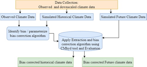
Climate bias correction methods aim to correct systematic errors, or biases, in climate model outputs by comparing them with observed climate data. The general methodology of climate bias correction methods: data collection, climate model simulation, bias assessment, bias correction method selection, bias correction implementation, evaluation and application were involved (Figure 4). According to Laux et al. (2021) data from the Global Circulation Model (GCM) may be skewed. Therefore, before being used for drought analysis, the models need to be modified. Linear-scaling approach (Teutschbein and Seibert 2012) was used for this study due to its simplicity and suitability for bias correction at the daily bias of precipitation and temperature data. Utilizing the CMhyd tool (https://swat.tamu.edu/software/cmhyd/), bias correction was completed before the implementation of the hydrological simulation model and drought analysis. Precipitation and temperature model data are corrected by the multiplier and additive terms, respectively. (4) $${\mathrm{T}}^{\mathrm{*}}\mathrm{ }\mathrm{GCM},\mathrm{daily}=\text{T GCM},\mathrm{daily}+({\mathrm{T}}^{-}\mathrm{o}\mathrm{b},\mathrm{daily}-{\mathrm{T}}^{-}\mathrm{G}\mathrm{CM},\mathrm{daily})$$(4) (5) $${\mathrm{P}}^{\mathrm{*}}\mathrm{ }\mathrm{GCM},\mathrm{daily}=\mathrm{PGCM},\mathrm{daily}\mathrm{\hspace{0.17em}*\hspace{0.17em}}\left(\frac{{\mathrm{P}}^{-}\mathrm{O}\mathrm{b},\mathrm{daily}}{{\mathrm{P}}^{-}\mathrm{G}\mathrm{CM},\mathrm{daily}}\right)$$(5)

Figure 4. General methodological frame work for bias correction of downscaled climate data (GCM).

where; T_GCM daily, is the daily GCM simulated temperature data, T_GCM, daily is the mean daily GCM simulated temperature for respective time horizons, T_ob daily is the mean daily observed temperature for the given time period, P_GCM, daily is the daily $\mathrm{GCM}$ simulated precipitation, P_ob daily is the mean daily observed precipitation for the given period and P GCM daily is the mean daily GCM simulated precipitation for respective time horizons.

Bias-corrected precipitation data plays a crucial role in ensuring that decisions, plans, and designs are based on reliable and realistic information for climate modeling, water resource management, flood forecasting and management, agricultural and crop planning, climate change assessment, infrastructural plan and design, research study (Masood and Takeuchi 2016: Salmoral et al. 2019: Quevauviller et al. 2012: Bhatti et al. 2023).

2.2.3. Evaluations of CMIP-6 climate model outputs

After bias correction, Global Climate Model data outputs were evaluated to select the best fit models for this study. Performances of twelve GCMs models were evaluated using statistical indicators. The statistics used for the evaluation of climate data sets were Root mean square Error (RMSE), Percent of bias (PBAIS), and correlation coefficients (r) which are also used for this study.

2.2.3.1. Root means square error (RMSE)

RMSE (Equation (8)(8) $$\mathrm{corrlation}\mathrm{ }\left(\mathrm{r}\right)=\frac{\mathrm{covariance}\mathrm{ }(\mathrm{simmulated},\mathrm{obsrved})}{\text{St simmulated*St obsrved}}$$(8) ) measures the difference between the distributions of the observed data and the distribution of historical data estimation, and calculates a weighted average error, weighted according to the square of the error. RMSE is useful when large errors are undesirable. The lower the RMSE score, the closer the historical data estimation represents the observed data measurement.

2.2.3.2. Percent of bias (PBAIS)

The PBIAS (Equation (7)(7) $$\text{Percent of Bais}=\frac{1}{\mathrm{n}}\sum {\left(\mathrm{S}\text{-}\mathrm{O}\right)}^2\mathrm{\times }100\mathrm{ }$$(7) ) measures the average tendency of the simulated values to be larger or smaller than their observed counterparts. The optimal value of PBIAS is zero. PBIAS is the deviation of data being evaluated, expressed as a percentage. A positive PBIAS value indicates the model is under–predicting measured values, whereas negative values indicate over predicting.

2.2.3.3. Correlation coefficients (r)

Correlation coefficient (r) (Equation (8)(8) $$\mathrm{corrlation}\mathrm{ }\left(\mathrm{r}\right)=\frac{\mathrm{covariance}\mathrm{ }(\mathrm{simmulated},\mathrm{obsrved})}{\text{St simmulated*St obsrved}}$$(8) ) is a measure of how closely the data in a regression line fit the data in the sample. r- value is close to 1, the better the fit. An r- value of 0 indicates that the regression line does not fit the data at all (GCM Climate data and observed data does not agree), while an r- value of 1 indicates a perfect fit. (6) $$\text{Root mean sequre error}=\sqrt{\frac{1}{\mathrm{n}}\sum {\left(\mathrm{S}\text{-}\mathrm{O}\right)}^2\mathrm{ }}$$(6) (7) $$\text{Percent of Bais}=\frac{1}{\mathrm{n}}\sum {\left(\mathrm{S}\text{-}\mathrm{O}\right)}^2\mathrm{\times }100\mathrm{ }$$(7) (8) $$\mathrm{corrlation}\mathrm{ }\left(\mathrm{r}\right)=\frac{\mathrm{covariance}\mathrm{ }(\mathrm{simmulated},\mathrm{obsrved})}{\text{St simmulated*St obsrved}}$$(8) where n is the number of samples, S is Simulated data recorded by climate model, O is observed data and St is standard deviation. Historical data were compared with observed rainfall, maximum temperature, and minimum temperature, for all global climate models.

2.2.3.4. Trend analysis of future temperatures and precipitation change

Various statistical techniques are used in studies that identify trends and other changes in climate and hydrological variables. Both parametric and nonparametric methods fall into this category. In contrast to non-parametric approaches, parametric methods presuppose a normal distribution of variables. The Mann-Kendall test is resilient against outliers, it does not require the elimination of outliers before trend discovery, and it does not make any assumptions about the distribution of the data (Takele et al. 2022). Hence, the Mann-Kendall nonparametric trend test by Mann (1945) and Kendall (1970) was used in this study. Trend analysis of precipitation and temperature data was evaluated using the Mann-Kendall trend test and Sen’s slope estimator by Mann (1945) and Kendall (1970) in XLSTAT 2014. The algorithm of this method is based on the principle that there is no significant trend if the calculated p-value is greater than the alpha value (0.05) (Arun et al. 2012). The statistic S is increased by 1, if the data value in the later period is greater than the data value in the earlier period. On the other hand, S is reduced by one if the data value sampled earlier is higher than the data value from a later period. The net result of all such increases and decreases yields the final value of S. Mann-Kendall S Statistics is computed as follows (9) $$S={\sum }_{i=1}^{n-1}{\sum }_{j=i+1}^n\mathit{sign}\mathrm{ }(X_j-X_i)$$(9) $$\mathit{sign}\left(X_j-X_i\right)=\{\begin{array}{c}1 if{\mathrm{ X}}_j-X_i>1 \\ 0 if{\mathrm{ X}}_j-X_i=1\\ -1 if{\mathrm{ X}}_j-X_i<1\end{array}$$

The upward or downward trend was shown by positive and negative values of S, respectively (Arun et al. 2012).

2.2.4. Soil and water assessment tool (SWAT) modeling

The SWAT model is a semi-distributed, physically based, and time-continuous hydrological model that was developed by the United States Department of Agriculture’s Agricultural Research Service. This model requires spatial data, meteorological variables, and hydrological data. SWAT simulates the streamflow based on the following water balance equation (Arnold et al. 1998). (10) $${\mathrm{SW}}_{\mathrm{t}}={\mathrm{SW}}_{\mathrm{o}}+\sum _{\mathrm{j}=1}^{\mathrm{t}}({\mathrm{R}}_{\mathrm{day}}-{\mathrm{Q}}_{\mathrm{surf}}\text{-}\mathrm{Ea}-{\mathrm{W}}_{\mathrm{seep}}-{\mathrm{Q}}_{\mathrm{gw}})$$(10) where SWt is the final soil water content (mm/day); SW_o is the initial water continent on day J (mm/day); t is the time in days; R_day is the amount of precipitation on the day j (mm/day); Q_surf is the amount of runoff on a day j (mm/day); Ea is amount of precipitation on day j (mm/day); W_seep is the amount of water entering the vadose zone from the soil profile on day j (mm/day) and Q_gw is the amount of return flow on day j (mm/day).

2.2.4.1. Sensitivity analysis, model calibration, and validation

Model sensitivity analysis, calibration, and validation were done by the SWAT Calibration and Uncertainty Fitting Program (SWAT-CUP). There are five algorithms in SWAT-CUP. SUFI-2 has gained the most popularity among users for carrying out parameterization, sensitivity analysis, calibration, validation, and uncertainty analysis of hydrological parameters (Saleh et al. 2000; Abbaspour et al. 2004) were used for this study. Model sensitivity analysis was used to select the most sensitive parameters that can affect the runoff formation of the case-study watershed. The best possible correspondence between observed and simulated runoff from a catchment must be determined by selecting model parameters. The total available observed flow data at the gauged station from 1985 to 2014 was used, with 20 years (1989–2006) for calibration and 9 years (2007–2014) for validation.

2.2.4.2. Model performance evaluation

Coefficient of determination (R²) (Krause et al. 2005), Nash-Sutcliffe efficiency (NSE) (Nash and Sutcliffe 1970), and percent of bias (Gupta et al. 1999) statistical parameters have been used to evaluate the SWAT model’s performance evaluation (Table 4). This is due to these statistical parameters being the most commonly used methods (Takele et al. 2022).

Table 4. The SWAT performance rate.

No.	Performance rating	NSE	R^2	PBIAS
1	Excellent	0.75 ˂ NSE ≤ 1.00	0.7 ˂ R2 ≤ 1.00	PBIAS ≤ ± 10
2	Good	0.65 ˂ NSE ≤ 0.75	0.6 ˂ R2 ≤ 0.7	± 10 ≤ PBIAS ˂ ± 15
3	Satisfactory	0.50 ˂NSE ≤ 0.65	0.50 ˂ R2 ≤ 0.6	±15 ≤ PBIAS ˂ ± 25
4	Unsatisfactory	NSE ≤ 0.50	R2 ≤ 0.50	PBIAS ≥ 25

(Source: Moriasi et al. 2007).

2.2.4.3. Nash-Sutcliffe efficiencies ($\mathit{NSE})$

Nash-Sutcliffe efficiencies ($\mathrm{NSE})$ range from infinity to one and are calculated by comparing the model’s goodness-of-fit to the variance of the observed data. The efficiency of one is equivalent to a perfect match between the modeled discharge and the measured data. It is defined as one minus the sum of the absolute squared differences between the predicted and observed values, normalized by the variance of the observed values during the period under investigation. $\mathrm{ }$ (11) $$\mathrm{NSE}=1-\frac{\sum \mathrm{ }{\left(\text{Simulated flow }\left(\mathrm{i}\right)-\text{Observed flow}\right)}^2\mathrm{ }\mathrm{ }}{\sum {\left(\text{Observed flow }\left(\mathrm{i}\right)-\text{Average of Observed average }\right)}^2\mathrm{ }}$$(11)

2.2.4.4. Coefficient of determination (R²)

The R² ranges between 0 and 1 which describes how much of the observed dispersion is explained by the prediction. A value of zero means no correlation at all whereas a value of 1 means that the dispersion of the prediction is equal to that of the observation. (12) $$\left({\mathrm{R}}^2\right)=1-\frac{\sum {\text{Simulated flow}-\text{Average simulated flow}\}}^2}{\sum {\left(\text{observed flow}-\text{Average observed flow}\right)}^2\mathrm{ }}$$(12)

2.2.4.5. Percent of bias (PBIAS)

The PBIAS measures the average tendency of the simulated values to be larger or smaller than their observed counterparts. The optimal value of PBIAS is zero. PBIAS is the deviation of data being evaluated, expressed as a percentage. A positive PBIAS value indicates the model is under–predicting measured values, whereas negative values indicate over predicting (Table 4). (13) $$\mathrm{PBIAS}=\sum \mathrm{ }\frac{\text{Simulated flow}-\text{observed flow})}{\text{Obseevd flow}}\mathrm{\times }100$$(13)

2.3. Drought index

The Drought Indices Calculator (DrinC) software was developed (Surendran et al. 2017; Tigkas et al. 2022) and addressed the drought characterization (Hydrological, Meteorological and Agricultural drought) based on indices, providing means for drought analysis based on drought indices for research and operational purposes (Tigkas et al. 2016). DrinC is a stand-alone software, freely available online (https://drought-software.com/, accessed on 29 April 2022) and it is currently used in more than 145 countries in a wide range of drought-related studies and applications (Tsakiris et al. 2016; Sobral et al. 2018; Shafeeque and Luo 2021; Yisehak et al. 2021). The primary benefits of the indexes, besides their uncomplicated framework and minimal data prerequisites, lie in their capacity to produce intelligible results that correspond to particular drought classifications, even for those who lack expertise in the subject matter.

2.3.1. Reconnaissance drought Index (RDI)

RDI is a recent drought analysis indicator which considers the effect of temperature in drought monitoring (Jain et al. 2015), Standard precipitation Index (SPI) only uses precipitation data, whereas RDI uses both precipitation and temperature as input data to overcome the limitation of SPI to understand the effect of temperature on water balance (Asadi Zarch et al. 2011). RDI computation is based on the ratio of total precipitation and potential evapotranspiration. The computation of RDI (Equation (15)) is based on the ratio of total precipitation (P) to potential evapotranspiration (PET) accumulated over the selected time scale (k) on the annual basis (k = 12) the classification of drought conditions is the same as SPI which ranges from −2 to 2, extreme drought to extreme wet, respectively (Table 5). (14) $$\alpha =\frac{\sum _{j=1}^{12}\mathit{Pij}}{\sum _{j=1}^{12}\mathit{PETij}}$$(14)

Table 5. Classification of drought index according to RDI, SDI, and aSPI values (McKee et al. 1993).

RDI, SDI and aSPI	Drought level
>2.00	Extremely wet
1.50 to 1.99	Very wet
1.00 to 1.49	Moderately wet
−0.99 to 0.99	Near Normal
−1.00 to −1.49	Moderate Drought
−1.50 to −1.99	Severe Drought
<−2	Extreme drought

with P_ij and PET_ij the precipitation and potential evapotranspiration of the j-_th month of the i-_th year

Therefore, the standardized RDI with α (alpha) version of the index (Equation (14)(14) $$\alpha =\frac{\sum _{j=1}^{12}\mathit{Pij}}{\sum _{j=1}^{12}\mathit{PETij}}$$(14) ) was computed following a similar procedure were used for the standardized precipitation index (SPI) computation (Tsakiris et al. 2007) and is given by (15) $${\mathit{RDI}}_{\left(k\right)}^{\left(i\right)}=\frac{y_{\left(k\right)}^{\left(i\right)}-{yk}^{-}}{\sigma yk}\text{With }{y}^{(i)}=\ln ({\alpha }^{\left(i\right)}$$(15) ${yk}^{-}\mathit{\text{ is }}$ arithmetic mean and $\sigma yk$ is Standardized deviation

And to calculate PET valve The Hargreaves equation (Buttafuoco et al. 2016) can be written as: (16) $$\mathit{PET}=0.0023Ra(T+17.8)\sqrt{(\mathit{Tmax}-\mathit{Tmin})}$$(16) where PET is the computed reference evapotranspiration (mm d⁻¹); Ra is the water equivalent of the extraterrestrial radiation (mm d⁻¹) computed according to Allen et al. (1998) T_max, T_min and ‘T’ are the daily maximum, minimum and mean air temperature (°C), with T calculated as the average of Tmax and Tmin. 0.0023 is the original empirical coefficient proposed by Hargreaves and Samani (1985).

2.3.2. Agricultural Standardized precipitation indices(aSPI)

The characterization of agricultural drought is focusing on the conditions affecting the development of vegetation, which is linked to the specific system under study (Tigkas et al. 2022). For instance, drought impacts may vary, depending on the considered plant species, the water deficits during critical growth stages, etc. Therefore, agricultural drought analysis should be based on properly adjustable tools, according to the properties of the system of interest. Despite advancements in the field of agricultural drought indices and despite the fact that crucial factors affecting plant development, such as soil moisture and evapotranspiration, are not taken into consideration, Standardized Precipitation Index (SPI) (McKee et al. 1993) is still the primary method for determining agricultural drought. This is mostly because to its straightforward structure and minimal data needs, which is significant for many places where only precipitation has access to sufficient time series or timely delivered data for operational purposes and the fact that it uses only precipitation data. Agricultural Standardized Precipitation Index (aSPI) (Tigkas et al. 2019), is proposed modified index, which is the most appropriate method for estimating the effective precipitation. The aSPI retains a similar standardization approach to SPI, through the fitting of the effective precipitation time series to a proper statistical distribution, which is then transformed into normal distribution. Many drought indices have been developed during the last decades for drought characterization and analysis. In this investigation, a modified version of SPI is proposed, namely the Agricultural Standardized Precipitation Index (aSPI), based on the substitution of the total precipitation by the effective precipitation, which describes more accurately the amount of water that can be used productively by the plants. The latter identifies agricultural drought better and successfully links drought severity to its effects on vegetation, especially in rainfed conditions.

The Standardized Precipitation Index (SPI) is a widely used index to characterize meteorological drought on a range of timescales. On short timescales, the SPI is closely related to soil moisture, while at longer timescales, the SPI can be related to groundwater and reservoir storage.

Agricultural Standardized Precipitation Index (aSPI), is proposed modified index, which is the most appropriate method for estimating the effective precipitation. The aSPI retains a similar standardization approach to SPI, through the fitting of the effective precipitation time series to a proper statistical distribution, which is then transformed into normal distribution.

If the gamma distribution is used, the probability density function is defined as (17) $$g\left(x\right)=\frac{1}{{\beta }^{\alpha }T\left(\alpha \right)}{X}^{\alpha -1e^{-x/\beta }}$$(17)

In which $\alpha$ is a shape parameter ($\alpha$>0), $\beta$ is a scale parameter ($\beta$>0), x is the effective precipitation value (x > 0) and I ($\alpha$) is the gamma function, expressed as ${\int }_0^{\infty }{y}^{\alpha -1}{e}^{-y}dy$

The parameter $\alpha$ and $\beta$ are estimated through the following formulation (Thom 1958). (18) $$\alpha =1+\sqrt{1+\frac{\frac{4A}{3}}{4A}}\mathrm{ }\beta =\frac{X^{\text{-}\mathrm{ }}}{\alpha }$$(18)

In which A = $Ln(x^{-}-\sum \frac{\ln \hspace{0.17em}\left(x\right)}{n}\mathrm{ }\mathit{and}\mathrm{ }n\mathrm{ }is\mathrm{ }\mathit{the}\mathrm{ }\mathit{number}\mathrm{ }of\mathrm{ }\mathit{obesrvations}.$

The cumulative probability G(x) of a precipitation event is (19) $$G\left(x\right)={\int }_0^{x}g\left(x\right)dx=\frac{{\int }_0^x{x}^{\alpha -1}{e}^{-\frac{x}{\beta }}dx}{{\beta }^{\alpha }T\left(\alpha \right)}$$(19) and letting t = x/β, Equation (11)(11) $$\mathrm{NSE}=1-\frac{\sum \mathrm{ }{\left(\text{Simulated flow }\left(\mathrm{i}\right)-\text{Observed flow}\right)}^2\mathrm{ }\mathrm{ }}{\sum {\left(\text{Observed flow }\left(\mathrm{i}\right)-\text{Average of Observed average }\right)}^2\mathrm{ }}$$(11) becomes the incomplete gamma function: (20) $$G\left(x\right)={\int }_0^x\frac{t^{\alpha -1}{e}^{-t}dt}{T\left(\alpha \right)}$$(20)

Given that gamma distribution is not defined for x = 0, the following formulation is used to account for the cumulative probability of zero effective precipitation (q) (Edwards 1997): (21) $$H\left(x\right)=q+\left(1-q\right)\mathrm{ }G\left(x\right)$$(21)

For the calculation of aSPI, the cumulative probability distribution is transformed into normal distribution using the following approximation (Abramowitz 1964): (22) $$\mathit{aSPI}=-(t-\frac{c0+c1t+c2t^2}{1+d1t+d2t^2+d3t^3},0<H(x)<0.5\text{ In which }t=\sqrt{\mathrm{l}\mathrm{n}(1/H{\left(x\right)}^2}$$(22)

$\mathit{aSPI}=(t-\frac{c0+c1t+c2t^2}{1+d1t+d2t^2+d3t^3},0.5<H(x)<1.0$ in which $t=\sqrt{\mathrm{l}\mathrm{n}(1/(1-H{\left(x\right)}^2}$ with the following constant values: $C0=2.515517,C1=0.802853,\mathrm{ }C2=0.010328\mathrm{ }d1=1.43278,d2=0.189269\mathrm{ }d3=0.001308$

2.3.3. Drought identification and characterizations

For the study, choosing the drought frequency, drought duration, drought magnitude and drought tendency, as the characteristic of drought events. In the identification of drought events, a drought event is defined as starting from the value of drought index greater than −0.99 (Near normal drought) until the drought index is less than −2 (extreme drought). The drought frequency is the ratio of the time of drought events to the total time series and the drought duration is the time of continuous occurrence of drought events. Drought events are identified based on drought indices values, according to Table 5 (McKee et al. 1993) and selected RDI, SDI and aSPI for both 6 and 12 months (RDI-6, RDI-12, SDI-6, SDI-12, aSPI-6 and aSPI-12) to reflect the annual drought.

2.3.4. Streamflow drought Index (SDI)

The Streamflow Drought Index (SDI) was calculated for the gauging stations for both the historical period and the future projections. The historical SDI was calculated based on observed streamflow data and for future projections simulated by the SWAT model. The SDI is based on the time series of monthly streamflow volumes (Qi,j), where i denotes the hydrological year and j is the month within that hydrological year (from October to September). Streamflow volume is calculated using the following equation: (23) $$Vi,k=\sum _{j=1}^{3k}Qi,k\mathrm{ }i=1,2,3\dots \dots \dots 12\mathrm{ }j=1,2,3\dots \dots .12\mathrm{ }k=1,2,3,4\mathrm{ }$$(23) where Vi,k is the cumulative streamflow volume for the i-th hydrological year and the k-th reference period, k = 1 for October–December, k = 2 for October–March, k = 3 for October–June, and k = 4 for October–September. The SDI is defined based on cumulative streamflow volumes Vi,k for each reference period k of the i-th hydrological year as follows: (24) $$\mathit{SDI}\mathrm{ }i,k\mathrm{ }=\frac{{Vi,k-Vk}^{-}}{\sigma k}\mathrm{ }i=1,2\mathrm{ }K=1,2,3,4$$(24) where V_k and S_k are, respectively, the mean and the standard deviation of cumulative streamflow volumes of the reference period k as these are estimated over a long period. Positive SDI values reflect wet conditions, while negative values indicate a hydrological drought. States of hydrological drought are defined by the SDI in an identical way to those used in the meteorological drought indices, such as the RDI (Zeng et al. 2015).

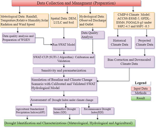
We considered three drought indices based on three categories of meteorological (RDI), hydrological (SDI) and agricultural (aSPI) drought in order to thoroughly evaluate future climate changes in long-term drought under different degrees of global warming. The flowchart for the modeling procedure is shown in Figure 5.

Figure 5. Flow chart of the study.

3. Result and discussion

3.1. Best fit CMIP-6 climate models

The best-fitted climate model outputs have been selected based on statistical indicators as stated in the method. It was selected from the 12 climate models. In Table 6, show that the RMSE value of ACCESS_ESM1-5 was 4.157, which means that lower the RMSE (closer the historical data estimation represents the observed data measurement). Similarly in Table 6, the value of correlation coefficient of FGOALS_g3 (0.634) was close to 1. i.e. the better the fit of observed and historical data. Generally, the ACCESS_ESM1-5, FGOALS_g3, and GFDL_ESM4 climate model outputs were selected due to having less RMSE (4.157, 7.177 and 7.311) and PBIAS (-0.547, −0.764 and −0.391) and a large correlation coefficient (0.634, 0.397 and 0.354) respectively.

Table 6. GCM output downscaled and selected models from CMIP-6 data sets.

Model type	RMSE	Correlation coefficient	PBIAS	Model type	RMSE	Correlation coefficient	PBIAS
FGOALS_g3	4.157	0.634	−0.547	IITM-ESM	9.047	0.314	−0.148
GFDL_ESM4	7.177	0.397	−0.764	BCC-CSM2-MR	9.672	0.298	−0.121
ACCESS_ESM1-5	7.311	0.354	−0.391	MPI-ESM1-2-LR	10.199	0.165	−0.063
MRI-ESM2-0	7.912	0.352	−0.063	INM-CM5-0	11.737	0.247	−0.063
MIROC6	8.281	0.349	−0.017	NESM3	12.107	0.340	−0.002
EC-Earth3	8.333	0.337	−0.065	MOCH_HadGEM3	12.346	0.307	−0.021

3.1.1. Trend analysis test for both base line and future temperature and precipitation

The projected future Rainfall and Temperature for the near term, the 2050s (2041–2070), and long term, the 2080s (2071–2100) time horizons were analyzed by Mann Kendall Trend, Therefore, the increasing trend will likely be the highest for the SSP5-8.5 and SSP2-4.5 scenario both for precipitation and temperature in the future shown on Figure 6 and Table 7.

Figure 6. Mann Kendall Trand test for preciptation (a) maximum Tempemprature (b) and minimum Tempemprature (c) both baseline and future scenario.

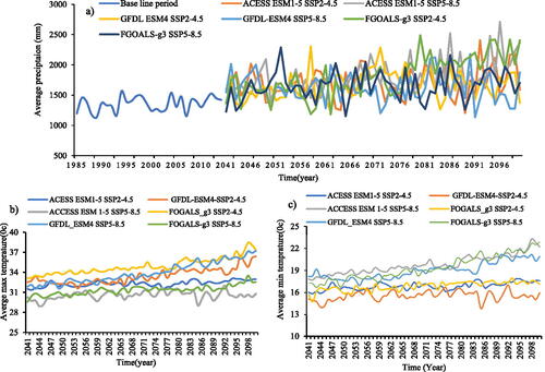
Table 7. Mann Kendall Trend test parameters for baseline and predicted precipitin and temperature.

Time	GCM models	SSPs Scenarios	Mann-Kendall Trend Test parameters
			Precipitation		Max. Temperature		Min. Temperature
			P-value	S	P-value	S	P-Value	S
2050s	ACCESS-ESM1-5	SSP2-4.5	0.98	2	0.89	2	0.89	24
		SSP5-8.5	0.34	11	0.28	126	0.28	13
	FOGALS-g3	SSP2-4.5	0.70	2	0.06	126	0.06	12
		SSP5-8.5	0.95	2	0.07	86	0.07	63
	GFDL-ESM4	SSP2-4.5	0.45	3	0.98	16	0.98	16
		SSP5-8.5	0.35	9	0.23	105	0.23	111
2080s	ACCESS-ESM1-5	SSP2-4.5	0.35	12	0.34	122	0.34	22
		SSP5-8.5	0.28	30	0.78	67	0.78	67
	FOGALS-g3	SSP2-4.5	0.70	20	0.67	45	0.67	45
		SSP5-8.5	0.23	23	0.23	2	0.23	118
	GFDL-ESM4	SSP2-4.5	0.50	50	0.07	12	0.07	12
		SSP5-8.5	0.45	70	0.08	82	0.08	38

3.2. Climate changes in precipitation

3.2.1. Annual, seasonal and monthly changes in projected rainfall

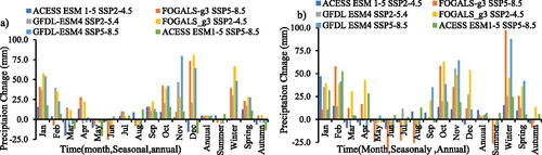
In the 2050s, mean annual precipitation may increase by 4.79% under SSP2-4.5 and 4.167% under SSP5-8.5 scenarios. In the 2080s, the relative change of projected precipitation may increase by 5.79% under SSP2-4.5 and 5.47% under SSP5-8.5 scenarios for three GCM climate outputs for ACCESS_ESM1-5, FGOALS_g3, GFDL_ESM4 respectively found on Figure 7.

Figure 7. Climate change impact on future precipitation under 2050s (a) and 2080s (b).

3.3. Climate change in projected temperature

3.3.1. Annual, seasonal and monthly changes in projected temperature

3.3.1.1. Maximum temperature

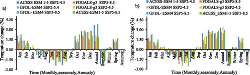
In the 2050s, the mean annual maximum temperature may increase by 2.51 °C under SSP2-4.5 and 2.31 °C under SSP5-8.5 scenarios. In the 2080s, the relative change of projected temperature may increase by 2.7 °C under SSP2-4.5 and 2.75 °C under SSP5-8.5 scenarios. for ACCESS_ESM1-5, FGOALS_g3, GFDL_ESM4 respectively (Figure 8).

Figure 8. Annual, seasonal, and monthly maximum temperature change (a) the 2050s and (b) the 2080s.

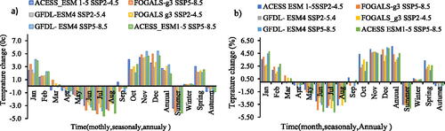
3.3.1.2. Minimum temperature

In the 2050s, the mean annual maximum temperature may increase by 2.69 °C under SSP2-4.5 and 2.54 °C under SSP5-8.5 scenarios. In the 2080s, the relative change of projected precipitation may increase by 4.11 °C under SSP2-4.5 and 4.25 °C under SSP5-8.5 scenarios for ACCESS_ESM1-5, FGOALS_g3, GFDL_ESM4 respectively, show in Figure 9.

Figure 9. Annual, seasonal, and monthly minimum temperature change (a) the 2050s and (b) the 2080s.

3.4. Hydrological modeling results

The total available observed river flow data at gauged stations from 1985 to 2014 was used for 20 years (1989–2006) with a two-year warming-up period for calibration and 9 years (2007–2014) for validation (Figure 10). Sensitivity analysis should be carried out to identify which parameter is most important for runoff formation. The t-test provides a measure of sensitivity, with a large value being more sensitive, and the p-value provides a measure of significance, for this study 12 Parameters were more sensitive and model performance indicators show in Table 8.

Figure 10. Hydrograph of simulated and observed flow for calibration (a) and validation (b) in daily calibration (c) and validation (d) in monthly.

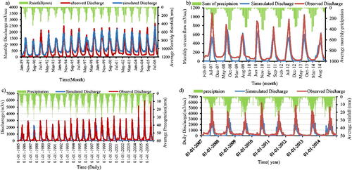
Table 8. Summary of statical model performance indictors from the above graph.

Hydrological Model Type	Daily Calibration		Monthly calibration
Soil and water assessment tool (SWAT)	R^2	NSE	R^2	NSE
	0.67	0.65	0.84	0.7

3.5. Climate changes impact on streamflow

3.5.1. Climate change impact on seasonal and annual flow volume

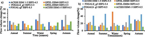
In order to predict how climate change may affect the socioeconomic situation in the Upper Blue Nile Basin at Kessie watershed, the effects of climate change on the seasonal and annual flow volume are were explored both scenarios (under 2050s and 2080s) shown Figure 11.

Figure 11. Percentage change in seasonal and annual flow volume (a) the 2050s and (b) 2080s.

3.6. Implications for future drought changes

3.6.1. Metrological drought characteristics using RDI

A meteorological drought analysis was conducted in the Kessie watershed using RDI from fourteen meteorological stations under climate change using the historical (1985–2014) and future (2041–2100) climate data with three ensemble GCM (ACCESS_ESM1-5, FGOALS_g3, GFDL_ESM4) both SSP2-4.5 and SSP5-8.5 scenarios. In the second step, the analysis of the indices RDI at multiple time scales (6 and 12 months) has been executed (Figure 12). The scale of 6 months for the drought in the medium term, and the scale of 12 months is used for the long-term drought. The magnitude, frequency and drought characteristics for RDI show in Table 9 and Figure 12. Table 9 shows that the Kessie watershed was regularly hit by severe and extreme meteorological droughts from historical (1985–2014) and future (2041–2100) climate change. The result also indicates that the magnitude and frequency of 2065s (-2.55, 0.7%), 2089s (-2.8, 1.83%) and 2090s (-2.61, 1.69%) was the most hazardous decade compared to other decades for Gundweyun, Gorgora and Werta stations, respectively. Spatially, more frequently drought occurred in the Bahir Dar (7.62% at 2059), Motta (13.25% at 2049), and Quarite (20.17% at 2063) stations compared to other stations (see Table 9). Generally, in the future the magnitude and trend of meteorological drought were increased. But, frequency of future metrological drought was lowered.

Figure 12. Metrological drought (RDI) for both base line period and future predicted scenario.

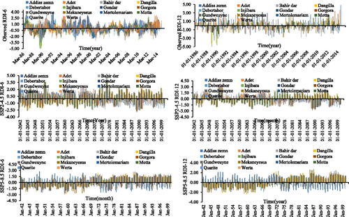
Table 9. Severe and extreme drought years (RDI12) in the Kessie watershed both SSP2-4.5 and SSP5-8.5.

Gauged Station GCM Scenarios		Drought year	Magnitude	Frequency (%)	Drought category
Addisse zemn	SSP2-4.5-RDI-12	2089	−2.27	1.41	Extreme
		2091	−1.98	5.22	Severe
	SSP5-8.5-RDI-12	2044	−1.90	5.92	Severe
		2067	−2.04	0.14	Extreme
Adet	SSP2-4.5-RDI-12	2090	−2.37	1.41	Extreme
		2091	−1.97	5.64	Severe
	SSP5-8.5-RDI-12	2051	−1.98	5.92	Severe
		2060	−2.39	1.55	Extreme
Bahir Dar	SSP2-4.5-RDI-12	2065	−1.99	7.34	Severe
		2090	−2.20	1.27	Extreme
	SSP5-8.5-RDI-12	2059	−1.98	7.62	Severe
		2060	−2.16	0.14	Extreme
Dangla	SSP2-4.5-RDI-12	2044	−1.97	2.1	Extreme
		2065	−2.31	5.07	Severe
	SSP5-8.5-RDI-12	2050	−1.99	3.95	Severe
		2060	−2.37	2.68	Extreme
Debertabor	SSP2-4.5-RDI-12	2089	−2.45	6.06	Severe
		2090	−1.98	2.82	Extreme
	SSP5-8.5-RDI-12	2077 2085	−1.91 −2.18	5.36 0.28	Severe Extreme
Injibara	SSP2-4.5-RDI-12	2051	−1.99	4.65	Severe
		2065	−2.47	0.85	Extreme
	SSP5-8.5-RDI-12	2062	−1.55	1.23	Severe
Gondar	SSP2-4.5-RDI-12	2051	−1.97	5.93	Severe
		2065	−2.38	1.84	Extreme
	SSP5-8.5-RDI-12	2092	−2.11	0.28	Extreme
		2093	−1.84	6.35	Severe
Gorgora	SSP2-4.5-RDI-12	2051	−1.99	5.93	Severe
		2089	−2.80	1.83	Extreme
	SSP5-8.5-RDI-12	2044	−1.50	0.14	Severe
Gundweyun	SSP2-4.5-RDI-12	2051	−1.90	5.4	Severe
		2065	−2.55	0.7	Extreme
	SSP5-8.5-RDI-12	2059	−1.55	0.98	Severe
Mekaneysus	SSP2-4.5-RDI-12	2051 2065	−1.92 −2.49	4.90 0.70	Severe Extreme
	SSP5-8.5-RDI-12	2060	−2.11	0.98	Extreme
		2063	−1.99	6.34	Severe
Mertomariam	SSP2-4.5-RDI-12	2080	−1.89	4.50	Severe
		2090	−2.47	1.55	Extreme
	SSP5-8.5-RDI-12	2044	−1.96	1.26	Extreme
		2060	−2.20	6.48	Severe
Motta	SSP2-4.5-RDI-12	2065	−1.90	1.83	Severe
		2089	−2.11	1.12	Extreme
	SSP5-8.5-RDI-12	2049	−1.13	13.25	Moderate
Quarite	SSP2-4.5-RDI-12	2051	−1.97	4.93	Severe
		2065	−2.53	0.70	Extreme
	SSP5-8.5-RDI-12	2063	−1.43	20.17	Severe
Werta	SSP2-4.5-RDI-12	2065	−1.87	2.96	Severe
		2090	−2.61	1.69	Extreme
	SSP5-8.5-RDI-12	2060	−1.69	3.52	Severe

3.6.2. Agricultural drought characteristics using aSPI

Agricultural drought analysis was computed using aSPI by considering fourteen meteorological stations under climate change using the historical (1985–2014) and future (2041–2100) climate data with three ensemble GCM (ACCESS_ESM1-5, FGOALS_g3, GFDL_ESM4) both SSP2-4.5 and SSP5-8.5 scenarios. Similar to RDI, the aSPI was computed for two-time scales (aSPI 6, and aSPI 12) depending on different season variations (Figure 13 and Table 10).

Figure 13. Agricultural drought analysis for both baseline and future predicted scenario data (aSPI).

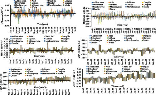
Table 10. Severe and extreme drought years (aSPI12) in the Kessie watershed both SSP2-4.5 and SSP5-8.5.

Stations GCM Scenarios		Drought year	Magnitude	Frequency (%)	Drought category
Addisszemne	SSP2-4.5-aSPI-12	2090	−2.82	1.84	Extreme
		2091	−1.97	3.24	Severe
	SSP5-8.5-aSPI-12	2044	−2.01	0.14	Extreme
		2067	−1.97	6.91	Severe
Adet	SSP2-4.5-aSPI-12	2065	−1.96	3.24	Severe
		2090	−2.75	2.11	Extreme
	SSP5-8.5-aSPI-12	2045	−1.99	6.35	Severe
		2059	−2.03	0.28	Extreme
Bahir Dar	SSP2-4.5-aSPI-12	2065	−1.96	4.09	Severe
		2089	−2.67	1.55	Extreme
	SSP5-8.5-aSPI-12	2050	−2.00	0.14	Extreme
		2063	−1.98	6.06	Severe
Dangla	SSP2-4.5-aSPI-12	2090	−2.92	1.97	Extreme
		2065	−1.99	3.53	Severe
	SSP5-8.5-aSPI-12	2050	−2.12	0.98	Extreme
		2060	−1.99	5.50	Severe
Debertabor	SSP2-4.5-aSPI-12	2051	−1.96	3.81	Severe
		2090	−2.71	1.82	Extreme
	SSP5-8.5-aSPI-12	2059	−1.98	6.63	Severe
		2063	−2.02	0.28	Extreme
Injibara	SSP2-4.5-aSPI-12	2065	−1.94	2.82	Severe
		2090	−2.91	2.25	Extreme
	SSP5-8.5-aSPI-12	2050	−2.07	1.13	Extreme
		2051	−1.96	5.35	Severe
Gondar	SSP2-4.5-aSPI-12	2051	−1.98	3.81	Severe
		2090	−2.80	6.35	Extreme
	SSP5-8.5-aSPI-12	2044	−2.05	0.7	Extreme
		2051	−1.98	6.35	Severe
Gorgora	SSP2-4.5-aSPI-12	2065	−1.98	3.95	Severe
		2090	−2.84	2.11	Extreme
	SSP5-8.5-aSPI-12	2044	−2.06	0.28	Extreme
		2050	−1.99	6.70	Severe
Gundweyun	SSP2-4.5-aSPI-12	2057	−1.88	3.67	Severe
		2090	−2.68	2.11	Extreme
	SSP5-8.5-aSPI-12	2063	−1.99	7.05	Severe
Mekaneysus	SSP2-4.5-aSPI-12	2065	−1.4	4.09	Moderate
		2090	−2.75	2.11	Extreme
	SSP5-8.5-aSPI-12	2045	−1.97	6.91	Extreme
Mertomariam	SSP2-4.5-aSPI-12	2090	−2.66	2.2	Extreme
		2091	−1.96	3.86	Severe
	SSP5-8.5-aSPI-12	2045	−1.95	6.77	Severe
		2060	−2.05	0.14	Extreme
Motta	SSP2-4.5-aSPI-12	2057	−1.98	3.59	Severe
		2090	−2.76	2.25	Extreme
	SSP5-8.5-aSPI-12	2062	−1.99	6.49	Severe
		2063	−2.04	0.423	Extreme
Quarite	SSP2-4.5-aSPI-12	2051	−1.97	4.93	Severe
		2090	−2.91	2.25	Extreme
	SSP5-8.5-aSPI-12	2063	−1.99	6.63	Severe
Werta	SSP2-4.5-aSPI-12	2065	−1.93	4.23	Severe
		2090	−2.63	1.69	Extreme
	SSP5-8.5-aSPI-12	2063	−2.01	0.14	Extreme

According to Table 10, based on historical (1985–2014) and projected (204–2100) climate change, the Kessie watershed was frequently affected by severe and extreme agricultural droughts. The result also indicates that the magnitude and frequency at 2090s were the most dangerous decade at SSP2-4.5 (aSPI12) for Dangla (-2.92,1,97%) and Injibara and Quarite (-2.91,2.25%). In comparison to other stations, the Addisszemne, Gundweyun, and Mekaneysus stations experienced drought more frequently in terms of location (Figure 13).

3.6.3. Hydrological drought characterization using SDI

The historical and future hydrologic droughts were analyzed using SDI at 6 and 12 month a time scale based on magnitude, frequency and drought characteristics (Figure 14 and Table 11). As shown in Table 11, six severe drought events and six extreme drought events occurred in Kessie station from a period of historical stream flow (1985–2014) and the three GCM ensemble with the Future (2041–2100) data. For SSP 5-8.5 (SDI-6) GCM Scenarios was highly affected by extreme drought. The frequency of severe drought is minimum at Observed (SDI-12) gauge stations. For the annual time scale (SDI12), severe and extreme drought events having that from 2045 (-3.03) at SSP5-8.5 and 2071(-3.28) at SSP2-4.5 for Kessie streamflow stations. The SSP2-4.5 scenario has a higher frequency hydrological drought at the Kessie gauge station indicates that the magnitude and frequency during 2044 (-1.93, 10.54%) and 2071 (-3.32, 6.93%,) on a monthly time scale (SDI6), whereas SSP 5-8.5 has higher magnitude at 2044 (-3.41, 4.47%) with low frequency. In Figure 6, SDI6, and SDI12 commonly showed that from 1985 to 1996, the Kessie observed stations was highly affected by hydrological drought for eleven consecutive years. Generally, after 1988, the hydrological drought severity in most stations of the basin decreased.

Figure 14. Hydrological drought index (SDI) analysis for baseline and future predicated scenario data.

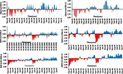
Table 11. Magnitude, drought year and frequency of hydrological drought (SDI).

Gauged Station	GCM Scenarios	Drought year	Magnitude	Frequency (%)	Drought category
Kessie	Observed SDI-6	1985	−1.98	3.01	Severe
		1988	−2.38	4.22	Extreme
	Observed SDI-12	1987	−1.94	1.72	Severe
		1988	−2.52	4.32	Extreme
Kessie	SSP 2-4.5 SDI-6	2044	−1.98	10.54	Severe
		2071	−3.32	6.93	Extreme
	SSP 5-8.5 SDI-6	2044	−3.41	4.47	Extreme
		2046	−1.94	4.32	Severe
Kessie	SSP2-4.5-SDI-12	2071	−3.28	4.08	Extreme
		2074	−1.86	5.03	Severe
	SSP 5-8.5-SDI-12	2045	−3.03	3.62	Extreme
		2071	−1.96	4.72	Severe

4. Discussion

According to this study, the Kessie Watershed’s climate has seen certain changes between 1985 and 2014 that have affected the region’s climate. All model outputs (ACCESS ESM1-5, FGOALS-g3, and GFDL-ESM4), in both scenarios (SSP2-4.5 and SSP5-8.5), and in the two-time horizons (the 2050s and the 2080s), predict an increase in the future mean annual precipitation, simulated streamflow, and mean annual temperature (both maximum and minimum temperatures) of the Kessie watershed. However, it appears illogical to increase streamflow as the temperature rises. Nevertheless, agriculture, which takes up around 59.25% of the total area in the case study watershed, is the predominant land use. It can result in higher runoff occurrence and lower infiltration rates. Additionally, the forest land has a very small area coverage, which results in less transpiration loss and interception. If both of these factors are present, the streamflow can be more affected by changes in precipitation than by changes in temperature in the case study watershed.

In all four seasons—summer, winter, spring, and autumn—the streamflow is anticipated to rise on a seasonal basis. In all model output data for both scenarios and time periods during winter and spring, maximum and minimum temperatures were found to be rising. Except for a very minor decline in the 2050s, both scenarios’ results for model output data from ACCESS_ESM1-5 reveal that precipitation also exhibits a rising tendency. Rainfall is predicted to grow rapidly (for example, it is predicted to increase up to 66.3% in the winter based on the FGOALS_g3 model output data in the 2050s on SPP2-4.5 scenario and up to 97% based on the FGOALS_g3 model output data in the 2080s on SPP5-8.5 scenario). However, the rate of temperature increase is not as rapid as the rate of precipitation; for instance, the highest maximum temperature change, according to the ACCESS ESM1-5 in SPP5-8.5 in the 2050s, was about 5.7%, and the highest maximum temperature change, according to the ACCESS ESM1-5 in SPP2-4.5 in the 2080s, was about 6.36%, both of which occurred in spring. The minimum temperature is rising, but not at the same rate as rainfall. In addition, because of the aforementioned factors, the model heavily depends on rainfall. Thus, rising temperatures in winter and spring and increased streamflow with rising rainfall may have resulted from these facts.

Previous study results in the upper Blue Nile Basin supports our findings. Extreme events, such meteorological, hydrological and Agricultural droughts, can be made worse by changes in temperature and precipitation. In many areas of Ethiopia, including the study region, drought is a recurrent occurrence. Devastating droughts have happened in the past ten years as the frequency of drought has grown across the nation (Bayissa et al. 2018; Mera 2018). According to Bayissa et al. (2015) there were severe hydrological droughts in the Abbay river basin in 1978/1979, 1984/1985, 1994/1995, and 2003/2004. Kebede et al. (2019) investigated that the years 1984, 2002, 2009, and 2015, including five weather stations and the entire Upper Blue Nile, show the highest intensity and longest length of drought in comparison to earlier meteorological drought periods. The result of this study also agreed with this finding, but there were some additional severe and extreme drought years such as 1985, 1987 and 1988 for historical dataset and 2044, 2045, 2046, 2071 and 2074 for future scenario (see Figure 10) in hydrological drought. For meteorological drought based on RDI the extreme drought years 2065s (-2.55), 2089s (-2.8) and 2090s (-2.61) were analyzed. Similar to hydrological and meteorological drought, agricultural drought was calculated using the aSPI, and the most harmful years were the intense drought years in the 2090s (-2.92). Typically, based on drought indicators like RDI, aSPI, and SDI compared to agricultural and meteorological droughts, hydrological droughts were more sensitive. This analysis was novel because it was conducted (1) using the most recent coupled model inter-comparison project phase 6 (CMIP-6) data outputs, (2) using the three model outputs that best fit the observed data (ACCESS_ESM1-5, FGOALS_g3, and GFDL_ESM4), which were chosen among the twelve models. (3) The SSP2-4.5 and SSP5-8.5 shared socioeconomic pathways were employed in the study, and (4) drought indicators such the RDI, SDI, and aSPI were used to analysis the hydrological, meteorological, and agricultural droughts. This was accomplished by creating drought indices that can quickly characterize and assess drought on various time frames. Therefore, water resource managers and decision-makers must plan and implement methods to reduce the negative effects of droughts, the efficient use of water resources, the timing of irrigation, and other human activities in the study region.

5. Conclusion

The goal of the study was to evaluate the performance of the new six-generation CMIP-6 climate output with two representative Shared socioeconomic pathways (SPP2-4.5 and SSP5-8.5) scenarios in order to assess how drought characteristics affected the climate change condition at the Kessie watershed, upper Blue Nile Basin, Ethiopia. Three of the best-fit models’ outputs are (ACESS_ESM1-5, GFDL_ESM4, and FOGALS_g3) because they fit the climate data outputs from GCMs the best when compared to the twelve climate output models’ observed data. Trend analysis of both base line and future temperature and precipitation was carried out by using the Mann-Kandel trend test and Sen’s slope estimator. The catchment hydrology was analyzed by the SWAT model through calibration and validation. The drought characteristics were done on the two-time horizons: the near term, 2050s (2041–2070), and the long term, 2080s (2071–2100) using hydrological (SDI), Meteorological (RDI) and Agricultural (aSPI) indicators. The observed data (1985–2014) were used as a reference period. The result revealed that precipitation and temperature are expected to slightly increase from the reference period to the long term based on all climate outputs data and both scenarios. Based on the yearly time scale, the results of the meteorological drought using RDI show that the years 2065s (-2.55, 0.7%), 2089s (-2.8, 1.83%) and 2090s (-2.61, 1.69%) were extremely dry, whereas agricultural droughts (aSPI) in 2090(-2.92, 1,97%) were the most extreme drought years. Similar to this, the hydrological drought (SDI) years of 2044 (-1.93, 10.54%), 2045 (-3.03, 3.62%), and 2071 (-3.32, 6.93%,) were exceptionally dry years. Short-term agricultural and hydrological droughts are also anticipated to occur more frequently. The projected increases in frequency and trend of agricultural and hydrological droughts in this area are greater due to the anticipated drop in annual rainfall and the larger increase in mean annual temperature in the middle of Kessie. These findings may be useful for water resources management and future planning for mitigation and adaptation to the climate change impact in the study area.

Author contributions

The study conception, design, material preparation, data collection and original draft of the manuscript were performed by A.E.A. A.B.N involved in writing, reviewing and editing the manuscript. A.Y.A and G.F.M were reviewed, supervising and commented the overall work from the beginning to the end. All authors read and approved the final manuscript.

Acknowledgments

We thank Wollo University, Kombolcha Institute of Technology (KIoT) for supporting and facilitating in this study.

Data availability statement

The data used in this study are primary and available after the authors were performed data collection and analysis.

Disclosure statement

No potential conflict of interest was reported by the authors.

References

- Abbaspour KC, Johnson CA, Van Genuchten MT. 2004. Estimating uncertain flow and transport parameters using a sequential uncertainty fitting procedure. Vadose Zone J. 3(4):1340–1352. doi: 10.2136/vzj2004.1340.
- Abramowitz M. 1964. Handbook of mathematical functions. National Bureau of Standards. Applied Mathematics Series, 55. https://cir.nii.ac.jp/crid/1572261549023928448
- AghaKouchak A, Farahmand A, Melton FS, Teixeira J, Anderson MC, Wardlow BD, Hain CR. 2015. Remote sensing of drought: progress, challenges and opportunities. Rev Geophys. 53(2):452–480. doi: 10.1002/2014RG000456.
- Ahmadalipour A, Moradkhani H. 2018. Multi-dimensional assessment of drought vulnerability in Africa: 1960–2100. Sci Total Environ. 644:520–535. doi: 10.1016/j.scitotenv.2018.07.023.
- Allen RG, Pereira LS, Raes D, Smith M. 1998. Crop evapotranspiration-Guidelines for computing crop water requirements-FAO Irrigation and drainage paper 56. Fao, Rome. 300(9):D05109.
- Arnold JG, Srinivasan R, Muttiah RS, Williams JR. 1998. Large area hydrologic modeling and assessment part I: model development. J Am Water Resour Assoc. 34(1):73–89. (doi: 10.1111/j.1752-1688.1998.tb05961.x.
- Arun M, Sananda K, Anirban M. 2012. Rainfall trend analysis by Mann-Kendall test: a case study of North-eastern part of Cuttack district. Int J Geol Earth Environ Sci. 2(1):70–78.
- Asadi Zarch MA, Malekinezhad H, Mobin MH, Dastorani MT, Kousari MR. 2011. Drought monitoring by reconnaissance drought index (RDI) in Iran. Water Resour Manage. 25(13):3485–3504. doi: 10.1007/s11269-011-9867-1.
- Asadi Zarch MA. 2022. Past and future global drought assessment. Water Resour Manage. 36(13):5259–5276. doi: 10.1007/s11269-022-03304-z.
- Bayissa Y, Maskey S, Tadesse T, Van Andel SJ, Moges S, Van Griensven A, Solomatine D. 2018. Comparison of the performance of six drought indices in characterizing historical drought for the upper Blue Nile basin, Ethiopia. Geosciences. 8(3):81. doi: 10.3390/geosciences8030081.
- Bayissa YA, Moges SA, Xuan Y, Van Andel SJ, Maskey S, Solomatine DP, Griensven AV, Tadesse T. 2015. Spatio-temporal assessment of meteorological drought under the influence of varying record length: the case of Upper Blue Nile Basin, Ethiopia. Hydrol Sci J. 60(11):1–16. doi: 10.1080/02626667.2015.1032291.
- Beguería S, Vicente‐Serrano SM, Reig F, Latorre B. 2014. Standardized precipitation evapotranspiration index (SPEI) revisited: parameter fitting, evapotranspiration models, tools, datasets and drought monitoring. Int J Climatol. 34(10):3001–3023. doi: 10.1002/joc.3887.
- Bhatti MT, Anwar AA, Hussain K. 2023. Characterization and outlook of climatic hazards in an agricultural area of Pakistan. Sci Rep. 13(1):9958. doi: 10.1038/s41598-023-36909-4.
- Buttafuoco G, Caloiero T, Guagliardi I, Ricca N. 2016. Drought assessment using the reconnaissance drought index (RDI) in a southern Italy region. In: Proceedings of the 6th IMEKO TC19 Symposium on Environmental Instrumentation and Measurements, Reggio Calabria, Italy, p. 24–25.
- Conway D. 2000. A water balance model of the Upper Blue Nile in Ethiopia. Hydrol Sci J. 42(2).
- Cook BI, Mankin JS, Anchukaitis KJ. 2018. Climate change and drought: from past to future. Curr Clim Change Rep. 4(2):164–179. doi: 10.1007/s40641-018-0093-2.
- Cook BI, Mankin JS, Marvel K, Williams AP, Smerdon JE, Anchukaitis KJ. 2020. Twenty‐first century drought projections in the CMIP6 forcing scenarios. Earth’s Future. 8(6):e2019EF001461.
- Edwards DC. 1997. Characteristics of 20th Century drought in the United States at multiple time scales. Air Force Inst of Tech Wright-Patterson Afb Oh. https://apps.dtic.mil/sti/citations/ADA325595
- Enyew BD, Van Lanen HAJ, Van Loon AF. 2014. Assessment of the impact of climate change on hydrological drought in Lake Tana catchment, Blue Nile basin, Ethiopia. J Geol Geosci. 3:174.
- Fang GH, Yang J, Chen YN, Zammit C. 2015. Comparing bias correction methods in downscaling meteorological variables for a hydrologic impact study in an arid area in China. Hydrol Earth Syst Sci. 19(6):2547–2559. doi: 10.5194/hess-19-2547-2015.
- Fujimori S, Hasegawa T, Masui T, Takahashi K, Herran DS, Dai H, Hijioka Y, Kainuma M. 2017. SSP3: AIM implementation of shared socioeconomic pathways. Global Environ Change. 42:268–283. doi: 10.1016/j.gloenvcha.2016.06.009.
- Gemeda DO, Sima AD. 2015. The impacts of climate change on African continent and the way forward. J Ecol Nat Environ. 7(10):256–262.
- Gupta HV, Sorooshian S, Yapo PO. 1999. Status of automatic calibration for hydrologic models: comparison with multilevel expert calibration. J Hydrol Eng. 4(2):135–143. doi: 10.1061/(ASCE)1084-0699(1999)4:2(135).
- Hargreaves GH, Samani ZA. 1985. Reference crop evapotranspiration from temperature. Appl Eng Agric. 1(2):96–99.
- Hay LE, Wilby RL, Leavesley GH. 2000. A comparison of delta change and downscaled GCM scenarios for three mountainous basins in the United States 1. J Am Water Resour Assoc. 36(2):387–397. doi: 10.1111/j.1752-1688.2000.tb04276.x.
- Hessl AE, Anchukaitis KJ, Jelsema C, Cook B, Byambasuren O, Leland C, Nachin B, Pederson N, Tian H, Hayles LA. 2018. Past and future drought in Mongolia. Sci Adv. 4(3):e1701832. doi: 10.1126/sciadv.1701832.
- IPCC. 2021. Climate change 2021: The physical science basis. In: Masson-Delmotte V, Zhai P, Pirani A, Connors SL, Péan C, Berger S, Caud N, Chen Y, Goldfarb L, Gomis MI, et al., editors. Contribution of working group I to the Sixth Assessment Report of the Intergovernmental Panel Climate Change. Cambridge, UK and New York, NY: Cambridge University Press. doi: 10.1017/9781009157896.
- Jain VK, Pandey RP, Jain MK, Byun H-R. 2015. Comparison of drought indices for appraisal of drought characteristics in the Ken River Basin. Weather Clim Extremes. 8:1–11. doi: 10.1016/j.wace.2015.05.002.
- Kebede A, Raju JP, Korecha D, Takele S, Nigussie M. 2019. Drought sensitivity characteristics and relationships between drought indices over Upper Blue Nile basin. J Water Land Dev. 43(1):64–75. doi: 10.2478/jwld-2019-0064.
- Krause P, Boyle DP, Bäse F. 2005. Comparison of different efficiency criteria for hydrological model assessment. Adv Geosci. 5:89–97. doi: 10.5194/adgeo-5-89-2005.
- Kusangaya S, Warburton ML, Van Garderen EA, Jewitt GPW. 2014. Impacts of climate change on water resources in southern Africa: a review. Phys Chem Earth, Parts a/b/c. 67–69:47–54. doi: 10.1016/j.pce.2013.09.014.
- Laux P, Rötter RP, Webber H, Dieng D, Rahimi J, Wei J, Faye B, Srivastava AK, Bliefernicht J, Adeyeri O, et al. 2021. To bias correct or not to bias correct? An agricultural impact modelers’ perspective on regional climate model data. Agric For Meteorol. 304–305:108406. doi: 10.1016/j.agrformet.2021.108406.
- Leander R, Buishand TA. 2007. Resampling of regional climate model output for the simulation of extreme river flows. J Hydrol. 332(3–4):487–496. doi: 10.1016/j.jhydrol.2006.08.006.
- Lenderink G, Van Ulden A, Van den Hurk B, Keller F. 2007. A study on combining global and regional climate model results for generating climate scenarios of temperature and precipitation for the Netherlands. Clim Dyn. 29(2–3):157–176. doi: 10.1007/s00382-007-0227-z.
- Levy SR, Migacheva K, Ramírez L, Okorodudu C, Cook H, Araujo‐Soares V, Minescu A, Livert D, Ragin DF, Walker P. 2022. A human rights based approach to the global children’s rights crisis: a call to action. J Soc Issues. 78(4):1085–1097. doi: 10.1111/josi.12563.
- Liu C, Yang C, Yang Q, Wang J. 2021. Spatiotemporal drought analysis by the standardized precipitation index (SPI) and standardized precipitation evapotranspiration index (SPEI) in Sichuan Province, China. Sci Rep. 11(1):1280. doi: 10.1038/s41598-020-80527-3.
- Livada I, Assimakopoulos VD. 2007. Spatial and temporal analysis of drought in Greece using the Standardized Precipitation Index (SPI). Theor Appl Climatol. 89(3–4):143–153. doi: 10.1007/s00704-005-0227-z.
- Lloyd-Hughes B. 2014. The impracticality of a universal drought definition. Theor Appl Climatol. 117(3–4):607–611. doi: 10.1007/s00704-013-1025-7.
- Loakes K. 2016. Late Quaternary palaeolimnology and environmental change in the South Wollo Highlands, Ethiopia [Doctoral dissertation]. Loughborough University.
- M’Po YN, Lawin AE, Oyerinde GT, Yao BK, Afouda AA. 2016. Comparison of daily precipitation bias correction methods based on four regional climate model outputs in Ouémé Basin, Benin. Hydrology. 4(6):58–71.
- Masood M, Takeuchi K. 2016. Climate change impacts and its implications on future water resource management in the Meghna Basin. Futures. 78–79:1–18. doi: 10.1016/j.futures.2016.03.001.
- McKee TB, Doesken NJ, Kleist J. 1993. The relationship of drought frequency and duration to time scales. In: Proceedings of the 8th Conference on Applied Climatology. Vol. 17, p. 179–183.
- Melaku MT. 2020. Social and political history of Wollo Province in Ethiopia: 1769–1916. https://etd.uwc.ac.za/handle/11394/7290
- Mera GA. 2018. Drought and its impacts in Ethiopia. Weather Clim Extremes. 22:24–35. doi: 10.1016/j.wace.2018.10.002.
- Moriasi DN, Arnold JG, Van Liew MW, Bingner RL, Harmel RD, Veith TL. (2007). Model evaluation guidelines for systematic quantification of accuracy in watershed simulations. Trans ASABE, 50(3), 885–900. doi: 10.13031/2013.23153.
- Nash JE, Sutcliffe JV. 1970. River flow forecasting through conceptual models, I: a discussion of principles. J Hydrol. 10(3):282–290. doi: 10.1016/0022-1694(70)90255-6.
- Nazarenko S, Kriaučiūnienė J, Šarauskienė D, Povilaitis A. 2023. The development of a hydrological drought index for Lithuania. Water. 15(8):1512. doi: 10.3390/w15081512.
- Nigussie AB, Tenfie HW, Zimale FA, Endalew A, Wudiye G. 2023. Evaluation of multiple bias correction methods with different satellite rainfall products in the Main Beles Watershed, Upper Blue Nile (Abbay) Basin, Ethiopia. J Water Clim Change. 14(1):156–174. doi: 10.2166/wcc.2022.244.
- Philip S, Kew SF, Jan van Oldenborgh G, Otto F, O’Keefe S, Haustein K, King A, Zegeye A, Eshetu Z, Hailemariam K, et al. 2018. Attribution analysis of the Ethiopian drought of 2015. J Clim. 31(6):2465–2486. doi: 10.1175/JCLI-D-17-0274.1.
- Quevauviller P, Barceló D, Beniston M, Djordjevic S, Harding RJ, Iglesias A, Ludwig R, Navarra A, Navarro Ortega A, Mark O, et al. 2012. Integration of research advances in modelling and monitoring in support of WFD river basin management planning in the context of climate change. Sci Total Environ. 440:167–177. doi: 10.1016/j.scitotenv.2012.07.055.
- Saleh A, Arnold JG, Gassman PW, Hauck LM, Rosenthal WD, Williams JR, McFarland AMS. 2000. Application of SWAT for the Upper North Bosque River Watershed. Trans Am Soc Agric Eng. 43(5):1077–1087. doi: 10.13031/2013.3000.
- Salmoral G, Rey D, Rudd A, Margon P, Holman I. 2019. A probabilistic risk assessment of the national economic impacts of regulatory drought management on irrigated agriculture. Earth’s Future. 7(2):178–196. doi: 10.1029/2018EF001092.
- Seager R, Osborn TJ, Kushnir Y, Simpson IR, Nakamura J, Liu H. 2019. Climate variability and change of Mediterranean-type climates. J Clim. 32(10):2887–2915. doi: 10.1175/JCLI-D-18-0472.1.
- Shafeeque M, Luo Y. 2021. A multi-perspective approach for selecting CMIP6 scenarios to project climate change impacts on glacio-hydrology with a case study in Upper Indus river basin. J Hydrol. 599:126466. doi: 10.1016/j.jhydrol.2021.126466.
- Sheffield J, Xia Y, Luo L, Wood EF, Ek M, Mitchell KE. 2012. North American Land Data Assimilation System: A framework for merging model and satellite data for improved drought monitoring.
- Sobral BS, Oliveira‐Júnior JF, de Gois G, Pereira‐Júnior ER. 2018. Spatial variability of SPI and RDIst drought indices applied to intense episodes of drought occurred in Rio de Janeiro State, Brazil. Int J Climatol. 38(10):3896–3916. doi: 10.1002/joc.5542.
- Surendran U, Kumar V, Ramasubramoniam S, Raja P. 2017. Development of drought indices for semi-arid region using drought indices calculator (DrinC)–a case study from Madurai District, a semi-arid region in India. Water Resour Manage. 31(11):3593–3605. doi: 10.1007/s11269-017-1687-5.
- Takele GS, Gebrie GS, Gebremariam AG, Engida AN. 2022. Future climate change and impacts on water resources in the Upper Blue Nile basin. Water Clim Change. 13(2):908–925. doi: 10.2166/wcc.2021.235.
- Tallaksen LM, Van Lanen HAJ. 2004. Hydrological drought: processes and estimation methods for streamflow and groundwater.
- Taye M, Sahlu D, Zaitchik BF, Neka M. 2020. Evaluation of satellite rainfall estimates for meteorological drought analysis over the upper Blue Nile basin, Ethiopia. Geosciences. 10(9):352. doi: 10.3390/geosciences10090352.
- Taye MA. 2021. Agro–ecosystem sensitivity to climate change over the Ethiopian highlands in a watershed of Lake Tana sub–basin. Heliyon. 7(7):e07454. doi: 10.1016/j.heliyon.2021.e07454.
- Teutschbein C, Seibert J. 2012. Bias correction of regional climate model simulations for hydrological climate-change impact studies: review and evaluation of different methods. J Hydrol. 456–457:12–29. doi: 10.1016/j.jhydrol.2012.05.052.
- Thom HCS. 1958. A note on the gamma distribution. Mon Weather Rev. 86(4):117–122. doi: 10.1175/1520-0493(1958)086<0117:ANOTGD>2.0.CO;2.
- Tigkas D, Vangelis H, Proutsos N, Tsakiris G. 2022. Incorporating aSPI and eRDI in drought indices calculator (DrinC) software for agricultural drought characterisation and monitoring. Hydrology. 9(6):100. doi: 10.3390/hydrology9060100.
- Tigkas D, Vangelis H, Tsakiris G. 2016. Introducing a modified reconnaissance drought index (RDIe) incorporating effective precipitation. Proc Eng. 162:332–339. doi: 10.1016/j.proeng.2016.11.072.
- Tigkas D, Vangelis H, Tsakiris G. 2019. Drought characterisation based on an agriculture-oriented standardised precipitation index. Theor Appl Climatol. 135(3–4):1435–1447. doi: 10.1007/s00704-018-2451-3.
- Tsakiris G, Kordalis N, Tigkas D, Tsakiris V, Vangelis H. 2016. Analysing drought severity and areal extent by 2D Archimedean copulas. Water Resour Manage. 30(15):5723–5735. doi: 10.1007/s11269-016-1543-z.
- Tsakiris G, Pangalou D, Vangelis H. 2007. Regional drought assessment based on the Reconnaissance Drought Index (RDI). Water Resour Manage. 21(5):821–833. doi: 10.1007/s11269-006-9105-4.
- Vithlani NS, Rank HD. 2016. Climate change impact assessment for Aji Basin using statistical downscaling and bias correction of climate model outputs. Curr World Environ. 11(2):670–678. doi: 10.12944/CWE.11.2.40.
- Wang T, Tu X, Singh VP, Chen X, Lin K. 2021. Global data assessment and analysis of drought characteristics based on CMIP6. J Hydrol. 596:126091. doi: 10.1016/j.jhydrol.2021.126091.
- Waseem M, Jaffry AH, Azam M, Ahmad I, Abbas A, Lee J-E. 2022. Spatiotemporal analysis of drought and agriculture standardized residual yield series nexuses across Punjab, Pakistan. Water. 14(3):496. doi: 10.3390/w14030496.
- Wilhite DA, Glantz MH. 1985. Understanding: the drought phenomenon: the role of definitions. Water Int. 10(3):111–120. doi: 10.1080/02508068508686328.
- Wood AW, Leung LR, Sridhar V, Lettenmaier DP. 2004. Hydrologic implications of dynamical and statistical approaches to downscaling climate model outputs. Clim Change. 62(1–3):189–216. doi: 10.1023/B:CLIM.0000013685.99609.9e.
- Yihdego Y, Vaheddoost B, Al-Weshah RA. 2019. Drought indices and indicators revisited. Arab J Geosci. 12(3):1–12. doi: 10.1007/s12517-019-4237-z.
- Yisehak B, Shiferaw H, Abrha H, Gebremedhin A, Hagos H, Adhana K, Bezabh T. 2021. Spatio‐temporal characteristics of meteorological drought under changing climate in semi‐arid region of northern Ethiopia. Environ Syst Res. 10(1):1–10. doi: 10.1186/s40068-021-00226-4.
- Yuan X, Zhang M, Wang L, Zhou T. 2017. Understanding and seasonal forecasting of hydrological drought in the Anthropocene. Hydrol Earth Syst Sci. 21(11):5477–5492.
- Zeng J, Li J, Lu X, Wei Z, Shangguan W, Zhang S, Dai Y, Zhang S. 2022. Assessment of global meteorological, hydrological and agricultural drought under future warming based on CMIP6. Atmos Oceanic Sci Lett. 15(1):100143. doi: 10.1016/j.aosl.2021.100143.
- Zeng X, Zhao N, Sun H, Ye L, Zhai J. 2015. Changes and relationships of climatic and hydrological droughts in the Jialing River Basin, China. PLoS One. 10(11):e0141648. doi: 10.1371/journal.pone.0141648.