Spatial enhanced spatiotemporal reflectance fusion model for heterogeneous regions with land cover change

Abstract

Numerous spatiotemporal fusion models have been developed to fuse dense time-series data with a high spatial resolution for monitoring land surface dynamics. Nonetheless, enhancing spatial details of fused images, eliminating the obvious ‘plaque’ phenomenon and image blurring in fused images, and developing relatively simple and¹ easy-to-implement algorithms remain a challenge for spatiotemporal fusion algorithms. Therefore, this paper presents a newly proposed spatial enhanced spatiotemporal reflectance fusion model (SE-STRFM) for image fusions in heterogeneous regions with land cover change. The SE-STRFM model predicts temporal changes of reflectance in sub-pixel details based on the spectral unmixing theory, and allocates reflectance changes caused by abrupt land cover change in fine-resolution images with a relatively simple algorithm and easy implementation. SE-STRFM only needs one pair of input data, comprising one fine-resolution image and one coarse-resolution image, to achieve high-precision reflectance prediction with spatial details. To verify the reliability and applicability of the SE-STRFM, we use Landsat image and simulated MODIS-like image to fuse high spatial and temporal resolution images and select two study areas with heterogeneous landscape and land cover type change for fusion experiments and accuracy evaluation. The results show that the images fused by SE-STRFM have clearer spatial details and a more accurate spectral distribution compared with those fused by the most widely used STARFM, ESTARFM and FSDAF. In two study areas with heterogeneous landscape and land cover type change, compared with STARFM, ESTARFM and FSDAF, the RMSE of SE-STRFM is 10.52%, 28.39% and 6.58% lower on average, respectively; r is 3.67%, 10.33% and 1.65% higher on average, respectively; AAD is 9.05%, 24.58% and 7.29% lower on average, respectively; and SSIM is 3.16%, 10.16% and 1.92% higher on average, respectively. SE-STRFM can accurately capture temporal changes with spatial details and effectively predict abrupt land-cover changes.

Keywords:

• Remote sensing
• spatiotemporal fusion
• spatial enhanced model
• heterogeneous landscape
• land cover change

1. Introduction

Remotely sensed data with high temporal and spatial resolution are of great significance in various applications, such as extracting land cover information (Gong et al. 2013, 2020) and monitoring land surface dynamics (Tran et al. 2016; Liu et al. 2020; Yang et al. 2020). However, owing to the compromise between satellite revisiting cycle and spatial resolution of sensors, as well as impacts of cloudy weather during remote sensing data acquisition, it is currently challenging to simultaneously obtain remote sensing data with both high spatial resolution and high revisiting frequency (Gao et al. 2006; Gevaert and García-Haro 2015; Zhu et al. 2018; Shi et al. 2022; Chen et al. 2023). For example, Landsat/SPOT images with 10–30 m spatial resolution are widely used for mapping large-scale land use and land cover change, but the nominal 16–26 day revisiting frequency and the effects of cloud contamination limit their use for monitoring land surface dynamics, crop growth, etc. (Ju and Roy 2008; Zhu et al. 2018). The Moderate Resolution Imaging Spectroradiometer (MODIS) on the Terra/Aqua satellite can achieve high-frequency imaging at the same location twice a day; however, its coarse spatial resolution (250 m to 1 km) cannot meet needs for land surface information extraction to enable quantitative applications in heterogeneous landscapes. Therefore, finding an effective way to fuse multi-source remote sensing data to construct dense time-series data with high spatial resolution is critical for multiple remote sensing applications, such as land cover mapping (Watts et al. 2011; Kong et al. 2016; Chen et al. 2017; Wang et al. 2017; Chen et al. 2023), land surface dynamic monitoring (Singh 2011; Zhang et al. 2014; Zhang, Huang, et al. 2015; Zhang, Zhang, et al. 2016; Tran et al. 2016; Ghosh et al. 2020; Yang et al. 2020), and crop growth and phenological changes detection (Gao et al. 2017), etc. To achieve this goal, a new domain of spatiotemporal image fusion has emerged in the last decade, focusing on blending multi-source remote sensing data with multi-resolution to produce synthetic images with both high spatial and temporal resolutions, thus enabling landscape and ecosystem processes monitoring (Gao et al. 2006; Zhu et al. 2018). Despite the recent emergence of satellite constellations and new satellite systems that can collect the latest satellite data (e.g. Sentinel-2 data with 10 m spatial resolution and 5 day revisiting frequency, and GF-1 WFV data with 16 m spatial resolution and 4 day revisiting frequency), spatiotemporal fusion is still necessary for these latest satellite data applications in areas with rainy and cloudy weather, or for long-term studies when using historical satellite images collected before 2015, such as Landsat/TM images to monitoring daily vegetation cover (Wu et al. 2018), estimating gross primary productivity (GPP) (Singh 2011), and generating daily land surface temperature and evapotranspiration (Weng et al. 2014; Semmens et al. 2016; Li et al. 2017) etc.

Numerous spatiotemporal fusion models have been developed based on specific principles (Zhang, Huang, et al. 2015; Zhu et al. 2018; Mariana and Alfred 2019; Cai et al. 2022). These models can be divided into five categories: unmixing-based models (Zhukov et al. 1999; Wu et al. 2012; Liu et al. 2020; Peng et al. 2022), weight function-based models (Gao et al. 2006; Hilker et al. 2009; Zhu et al. 2010), machine learning-based models (Huang and Song 2012; Moosavi et al. 2015; Wu et al. 2015), Bayesian-based models (Li et al. 2013; Liao et al. 2016), and hybrid models (Gevaert and García-Haro 2015; Zhu et al. 2016; Li et al. 2020). Among them, the Spatial and Temporal Adaptive Reflectance Fusion Model (STARFM) proposed by Gao et al. (2006) is one of the earliest and most widely used weight function-based spatiotemporal fusion models. The STARFM is theoretically based on the assumption that the spectral changes of fine-resolution images are consistent with those of coarse-resolution images at the same location, fusing image with the spatial resolution of Landsat and temporal frequency of MODIS (Gao et al. 2006). Although the STARFM is a simple, easy to implement, and widely used spatiotemporal fusion model, it has two primary shortcomings that need to be addressed for applications. First, the STARFM cannot accurately predict the reflectance of heterogeneous areas (Gao et al. 2006; Zhu et al. 2010). Second, the STARFM cannot predict reflectance changes caused by abrupt land cover changes (Hilker et al. 2009; Zhu et al. 2016, 2018). To address the issues mentioned above, a series of improved models of the STARFM have been developed based on various relevant principles. There are three main types of improvements, referred to herein as the STARFM family models: spatial improved-type models, temporal improved-type models, and spatiotemporal improved-type models.

The spatial improved-type models in the STARFM-family are primarily concerned with the impact of spatial heterogeneity on predicted reflectance. The existing spatial improved-type models such as the enhanced STARFM (ESTARFM) (Zhu et al. 2010), the modified version of ESTARFM (mESTARFM) (Fu et al. 2013), and the improved ESTARFM (IESTARFM) (Liu et al. 2019) improve the fusion effect in the spatial heterogeneity in a certain extent. The temporal improved-type models in the STARFM-family are primarily concerned with the impact of abrupt land cover changes on predicted reflectance. The Spatial Temporal Adaptive Algorithm for mapping Reflectance Change (STAARCH) proposed by Hilker et al. (2009) is a typical temporal improved-type model. By choosing optimal fine-resolution base data, the STAARCH model can effectively detect abrupt surface disturbances in forests. Nowadays, many spatiotemporal improved-type models have recently been developed in the STARFM family for effectively predicting the reflectance change caused by spatial heterogeneity and abrupt land-cover changes simultaneously. The spatiotemporal improved-type models have attracted much attention. The representative one is the Flexible Spatiotemporal Data Fusion (FSDAF) (Zhu et al. 2016) followed by its improved versions, such as optimized version of FSDAF (FSDAF 2.0) (Guo et al. 2020), the improved FSDAF (IFSDAF) (Liu et al. 2019), the enhanced Flexible Spatiotemporal DAta Fusion (SFSDAF) (Li et al. 2020), and Adaptive-SFSDAF (Hou et al. 2020). The newly proposed spatiotemporal improved-type models are the Reliable and Adaptive Spatiotemporal Data Fusion (RASDF) (Shi et al. 2022), and the Variation-based Spatiotemporal Data Fusion (VSDF) (Chen et al. 2022). Among spatiotemporal improved-type models, the FSDAF and its variants have been the fastest growing spatiotemporal improved-type models in the STARFM family in recent years. Although the FSDAF and its variant models can predict temporal and abrupt reflectance changes and present superior predictions relative to existing models, none of these methods has reached maturity. They have certain shortcomings as follows.

First, most existing FSDAF and its variant models can only predict phenological changes by processing at the pixel level, which results in visible ‘plaque’ phenomenon and image blurring in fused images by using the FSDAF and its variants.

Second, to predict the abrupt reflectance change caused by land-cover changes, most existing FSDAF and its variant models use the reflectance residuals by using the TPS interpolator (Zhu et al. 2016; Guo et al. 2020). However, the residual distribution obtained using the TPS interpolator relies entirely on the assumption that errors mainly depend on landscape homogeneity, which results in the blurring of fused images to some extent. Although the fusion accuracy has been improved to capture the abrupt land-cover changes to a certain extent with the development of spatiotemporal improved-type models in the STARFM family, these improved models such as SFSDAF, Adaptive-SFSDAF, RASDF, VSDF have become more complex with more parameters, which increase uncertainty and decrease the ease implementation of model applications, especially in large-scale image fusion applications (Gao et al. 2022; Chen et al. 2023). The STARFM family models developed based on different principles, especially the FSDAF and its variants, have various strengths and weaknesses, as mentioned above, and have partially solved the problem caused by spatial heterogeneities and abrupt land-cover class changes in spatiotemporal fusion. However, challenges related to fusion image quality and fusion model implementation persist, including the need to improve the spatial details of fused images, eliminate the obvious ‘plaque’ phenomenon, image blurring in fused images, and develop relatively simple and easy-to-implement algorithms.

To address the aforementioned limitations, it is necessary to develop spatially enhanced spatiotemporal fusion models by processing at the sub-pixel level to enhance the spatial details of fused images. The primary objective of this study is to develop a Spatial Enhanced Spatiotemporal Reflectance Fusion Model (SE-STRFM) that captures both temporal changes with spatial details by processing at the sub-pixel level and abrupt land cover changes. The SE-STRFM can predict both temporal changes with spatial details and abrupt land cover changes for heterogeneous regions with land-cover changes. Moreover, the proposed method requires only minimal input datasets, that is, one fine image and two coarse images.

In this paper, Landsat and MODIS-like images are adopted as input fine- and coarse-resolution images, respectively. The most widely used spatiotemporal image fusion benchmark models, including STARFM, ESTARFM and FSDAF, are used for comparison. In the second section of this paper, we introduce the theoretical basis, and the third section clarifies the steps of the SE-STRFM. The experimental data and accuracy evaluation methods are described in the fourth section. In Section 5, we examine the fusion results of the SE-STRFM and compare them with the STARFM, the ESTARFM and the FSDAF models. Finally, a discussion of the advantages and limitations of the SE-STRFM is presented.

2. Theoretical basis of the SE-STRFM

To enhance the spatial details and eliminate the plaque effect of fused images, the SE-STRFM model is proposed to predict fine-resolution images on the sub-pixel scale using the spectral unmixing theory (Ridd 1995; Small 2003, 2004; Wang et al. 2021). In general, most pixels in fine- or coarse-resolution images are mixed. In the same area, there are equal numbers and the same type of endmembers in both fine- and coarse-resolution images obtained simultaneously. Therefore, the relationship between the endmember reflectance of fine- and coarse-resolution image pixels can be expressed as (1) $$\mathrm{r}\left(k,{b,t}_n\right)=\mathrm{R}\left(k,{b,t}_n\right)+{\epsilon }_n$$(1) where r and R represent the reflectance of the kth endmember in fine- and coarse-resolution images, respectively, $b$ is the image band, $t_n$ is the acquisition date, and ${\epsilon }_n$ is the coefficient representing the systematic error caused by the sensor difference.

Assuming ${\epsilon }_n$ has no change from $t_1$ to $t_p,$ that is, $\mathrm{ }{\epsilon }_1={\epsilon }_p,$ the reflectance change of the endmember from $t_1$ to $t_p$ that mainly caused by phenological change and crop rotation without considering land cover type change (deforestation and urbanization) can be expressed as (2) $$\Delta \mathrm{r}\left(\mathrm{k},\mathrm{b},t_{1-p}\right)=\Delta \mathrm{R}\left(\mathrm{k},\mathrm{b},{\mathrm{t}}_{1\text{-}\mathrm{p}}\right)$$(2) where $\Delta \mathrm{r}$ and $\Delta R$ represent the reflectance changes of the kth endmember in the fine- and coarse-resolution image band $\mathrm{b}$ from $t_1$ to $t_p,$ respectively.

Assuming that there is no land cover change from $t_1$ to $t_p,$ the abundance of the k-th endmember in the fine-resolution image of band b does not change from $t_1$ to $t_p,$ that is, $f^k\left(x_{ij},y_{ij},{ b,t}_p\right)$ is equal to $f^k\left(x_{ij},y_{ij},{ b,t}_1\right).$ Among the mixing models, the linear mixture model is employed in this research for spectral unmixing, which is a simple but effective method (Lu et al. 2004; Jafarzadeh and Hasanlou 2019). Therefore, according to the linear spectral mixing theory, the predicted reflectance change of the fine-resolution pixel from $t_1$ to $t_p$ can be expressed as (3) $$\Delta L\left(x_{ij},y_{ij},b,t_{1-p}\right)=\sum {\mathrm{f}}^k\left(x_{ij},y_{ij},b,t_1\right)\Delta r\left(k,b,t_{1-p}\right)=\sum f^k\left(x_{ij},y_{ij},\mathrm{b},t_1\right)\Delta R(k,b,t_{1-p})$$(3)

By estimating the endmember abundance in fine-resolution images, $f^k\left(x_{ij},y_{ij},\mathrm{b},t_1\right)$ and the reflectance change of endmembers in coarse-resolution images from $t_1$ to ${ t}_p,$ $\Delta R(k,b,t_{1-p}),$ we can obtain the predicted reflectance change of a fine-resolution pixel from $t_1$ to $t_p,$ $\Delta L(x_{ij},y_{ij},b,t_{1-p}),$ under the condition of no land cover change from $t_1$ to $t_p.$

When land cover changes from $t_1$ to $t_p,$ the predicted reflectance change of the fine-resolution pixel from $t_1$ to $t_p$ is inaccurate. If the residuals, $\mathrm{q}\left(x_{ij},y_{ij},\mathrm{b},t_{1\text{-}\mathrm{p}}\right),$ caused by land cover changes can be calculated, the final predicted reflectance of fine-resolution pixels at $t_p$ can be obtained as (4) $$L\left(x_{ij},y_{ij},{b,t}_p\right)=L\left(x_{ij},y_{ij},\mathrm{b},t_1\right)+\Delta L\left(x_{ij},y_{ij},{b,t}_{1-p}\right)+\mathrm{q}\left(x_{ij},y_{ij},\mathrm{b},t_{1\text{-}\mathrm{p}}\right)$$(4)

3. Implementation of SE-STRFM

Based on the above theoretical basis, the SE-STRFM first predicts the reflectance of fine resolution with more spatial details in sub-pixel level assuming no land cover change during the prediction period, then the residuals caused by land cover change are estimated, and finally the predicted reflectance of the fine-resolution pixel at ${\mathrm{t}}_{\mathrm{p}}$ is obtained.

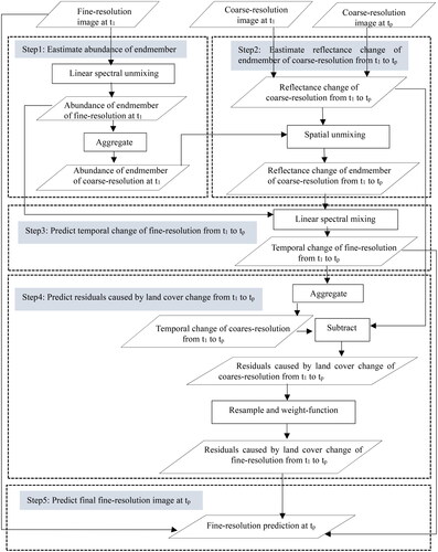
The SE-STRFM requires one fine-resolution image acquired at $t_1$ and two coarse-resolution images acquired at $t_1$ and $t_p$ as input data to fuse the fine-resolution image at $t_p.$ The input data preprocessing for radiometric calibration, atmospheric correction, and geometric registration is necessary before implementing the SE-STRFM. The implementation of the SE-STRFM mainly includes five steps: (1) estimating the endmember abundance of fine-resolution images at $t_1;$ (2) estimating the spectral reflectance change of the endmember in coarse-resolution images from $t_1$ to $t_p;$ (3) predicting the temporal change of fine-resolution pixels; (4) predicting the residuals of reflectance caused by land cover change at a fine resolution; and (5) obtaining final prediction images by adding predicted temporal change and allocated residuals to the preliminary image. A detailed description of each step in the SE-STRFM is shown in Figure 1.

Figure 1. Flowchart of SE-STRFM.

3.1. Estimating the endmember abundance of fine-resolution images

The abundance of endmembers of the fine-resolution image pixel at $t_1$ is estimated at the sub-pixel level using spectral mixture analysis. The implementation of the unmixing process includs the following steps.

1. Transforming the bands of fine-resolution images using minimum noise transformation (MNF). To reduce the correlation between the original bands of fine-resolution images, the bands of fine-resolution images are transformed using the MNF to a few principal components (bands) that concentrate the main information of the original bands of fine-resolution images.

2. Determination of spectral endmember. First, considering the surface complexity and spatial heterogeneity, we chose endmember types based on land cover characteristics in study area and the Low albedo-High albedo-Vegetation-Soil (L-H-V-S) model that describes that the land cover is primarily composed by land cover component with low albedo, land cover component with high albedo, vegetation and soil. Previous studies have demonstrated that the L-H-V-S model is more capable of describing land cover components than the Impervious-Vegetation-Soil (I-V-S) model to parameterize biophysical composition of land surface (Small 2003; Wu and Murray 2003; Somers et al. 2011). We then calculated the pixel purity index (PPI) in the feature space composed of the first three principal components and selected L-H-V-S endmembers from images using PPI to avoid the subjective influence of visual selection.

3. Estimation of the abundance of endmembers. The abundance of endmember is estimated through fully constrained spectral mixture analysis model using fine-resolution images at $t_1.$ The basic expression for linear spectral mixture analysis model is as follows: (5) $$L\left(x_{ij},y_{ij},t_1,b\right)=\sum _{k=1}^K{f}^k\left(x_{ij},y_{ij},b\right)r\left(k,b\right)+e_b$$(5) (6) $${\sum }_{k=1}^K{f}^k\left(x_{ij},y_{ij},b\right)=1$$(6) (7) $$0\le f^k\left(x_{ij},y_{ij},b\right)\le 1$$(7) (8) $$\mathit{RMSE}={\left(\frac{\sum _{b=1}^B{e_b}^2}{B}\right)}^{1/2}$$(8)

where $L$ is the reflectance of the fine-resolution pixel, $\left(x_{ij},y_{ij}\right)$ is the pixel coordinate of the fine-resolution pixel, $t_1$ is the image acquisition date, $b$ is the band, $k$ is the number of endmembers, $f^k$ is the abundance of the kth endmember, $r$ is the reflectance of endmember, $e_{\mathrm{b}}$ is the residual error, and $B$ is the number of bands. The endmember abundance can be determined using the least squares method to minimize the root mean square error (RMSE) of the model.

Using the abundance of endmembers in the fine-resolution image at $t_1,$ we can calculate the abundance of endmembers within a coarse pixel: (9) $${\mathrm{ }F}^k\left(X_i,Y_i,b,t_1\right)=\frac{1}{m}\sum _{j=1}^m{f}^k\left(x_{ij},y_{ij},b,t_1\right)$$(9) where $m$ is the number of fine pixels belonging to the kth endmember within the coarse pixel. The abundance of endmembers in coarse-resolution aggregated from the fine-resolution will average out some errors in spectral unmixing process.

3.2. Estimating the reflectance change of endmembers in coarse-resolution images

The reflectance change in the coarse-resolution image from $t_1$ to $t_p$ was calculated as follows: (10) $$\Delta M\left(X_i,Y_j,\mathrm{b},t_{1-p}\right)=M\left(X_i,Y_j,\mathrm{b},t_p\right)-M\left(X_i,Y_j,\mathrm{b}{,t}_1\right)$$(10) where $\Delta M$ is the change in the reflectance of the coarse-resolution pixel from $t_1$ to $t_p,$ $M$ is the reflectance of the coarse-resolution pixel, $\left(X_i,Y_i\right)$ are the coordinates of the coarse-resolution pixel, and $b$ is the image band.

According to the linear spectral mixing theory, the reflectance change of a coarse-resolution pixel is the sum of the endmember reflectance changes weighted by the corresponding endmember abundance: (11) $$\Delta M\left(X_i,Y_i,b,t_{1-p}\right)=\sum _{k=1}^K{F}^k\left(X_i,Y_i,b,t_1\right)\Delta R\left(k,b,t_{1-p}\right)+\mathrm{\delta }$$(11) where $\Delta R$ is the reflectance change of the kth endmember for band b from $t_1$ to $t_p$ and $\mathrm{\delta }$ is the residual of each coarse-resolution pixel.

The reflectance change of each endmember, $\Delta R\left(k,b,t_{1-p}\right),$ can be obtained by inversing Equation (11)(11) $$\Delta M\left(X_i,Y_i,b,t_{1-p}\right)=\sum _{k=1}^K{F}^k\left(X_i,Y_i,b,t_1\right)\Delta R\left(k,b,t_{1-p}\right)+\mathrm{\delta }$$(11) using the least squares method. However, $\Delta R\left(k,b,t_{1-p}\right)$ cannot be solved within a single coarse-resolution pixel because the number of unknowns is greater than one. If all coarse-resolution pixels in the entire image are used to solve this problem, the $\Delta R\left(k,b,t_{1-p}\right)$ may be over-averaged. Therefore, coarse-resolution pixels biger than K (the number of endmembers) are selected by using a certain size search window. By using $\omega \times \omega$ pixels in the search window, the $\Delta R\left(k,b,t_{1-p}\right)$ for the central pixel within the search window can be inversed continuously, step-by-step, to inverse by using Equation in (12) and the least-squares method. In order to minimize the impacts of collinearity and endmember reflectance changes in spatial unmixing process, we used 25 × 25 pixels in the search window according to literature (Liu et al. 2020) and our experiments. (12) $$\left[\begin{array}{c}\Delta M\left(X_1,Y_1,b,t_{1-p}\right)\\ ⋮\\ \Delta M\left(X_i,Y_i,b,t_{1-p}\right)\\ ⋮\\ \Delta M\left(X_n,Y_n,b,t_{1-p}\right)\end{array}\right]=\left[\begin{array}{c}{F}^1\left(X_i,Y_i,b\right)\cdots F^k\left(X_i,Y_i,b\right)\cdots F^K\left(X_i,Y_i,b\right)\\ ⋮\\ F^1\left(X_i,Y_i,b\right)\cdots F^k\left(X_i,Y_i,b\right)\cdots F^K\left(X_i,Y_i,b\right)\\ ⋮\\ F^1\left(X_n,Y_n,b\right)\cdots F^k\left(X_n,Y_n,b\right)\cdots F^K\left(X_n,Y_n,b\right)\end{array}\right]\left[\begin{array}{c}\Delta R\left(1,b,t_{1-p}\right)\\ ⋮\\ \Delta R\left(k,b,t_{1-p}\right)\\ ⋮\\ \Delta R\left(K,b,t_{1-p}\right)\end{array}\right]+\left[\begin{array}{c}\delta \left(X_1{Y}_1\right)\\ ⋮\\ \delta \left(X_i{Y}_i\right)\\ ⋮\\ \delta \left(X_n{Y}_n\right)\end{array}\right]$$(12) where $K$ indicates the number of endmembers and $n$ refers to the number of pixels in the moving window.

3.3. Predicting the temporal change of fine-resolution images

It is assumed that the endmember types and corresponding abundance of fine-resolution pixels remain unchanged when there is no land cover change from $t_1$ to $t_p.$ Therefore, the temporal change in fine-resolution pixels can be expressed as the sum of endmember reflectance changes weighted by the corresponding endmember abundance at $t_1$ (13) $$\Delta L\left(x_{ij},y_{ij},{b,t}_{1-p}\right)=\sum f^k\left(x_{ij},y_{ij},\mathrm{b}{,t}_1\right)\Delta r(k,b,t_{1\text{-}\mathrm{p}})$$(13) where $\Delta r\left(k,b,t_{1-p}\right)$ is the temporal change in the endmember reflectance within the fine-resolution pixel from $t_1$ to $t_p.$

According to Equation in (2) and (13), the temporal change in fine-resolution pixels can be expressed as (14) $$\Delta L\left(x_{ij},y_{i\mathrm{j}},{b,t}_{1-p}\right)=\sum f^k\left(x_{ij},y_{ij},\mathrm{b}{,t}_1\right)\Delta R(k,b,t_{1-p})$$(14)

3.4. Predicting residuals caused by land cover changes

3.4.1. Calculating residuals caused by land-cover changes

By neglecting geometric rectification errors and differences in atmospheric correction, the reflectance of a coarse-resolution pixel at $t_{\mathrm{n}}$ can be expressed as the sum of the reflectance of fine-resolution pixels within the coarse-resolution pixel. (15) $$M\left(X_i,Y_i,{b,t}_{\mathrm{n}}\right)=\frac{1}{m}\sum _{j=1}^{m}L\left(x_{ij},y_{ij},{b,t}_n\right)+\xi$$(15) where $M\left(X_i,Y_i,b{,t}_{\mathrm{n}}\right)$ is the reflectance of a coarse-resolution pixel at $\mathrm{ }{t}_{\mathrm{n}}$ band b; $L\left(x_{ij},y_{ij},b,t_n\right)$ is the reflectance of fine-resolution pixel at $\mathrm{ }{t}_{\mathrm{n}}$ band b, $m$ is the number of fine-resolution pixels within the coarse-resolution pixel, and $\xi$ is the system difference between two sensor systems caused by differences in bandwidth, acquisition time, and spectral response function. Assuming that the system difference does not change from $t_1$ to $t_p,$ the reflectance changes $\Delta M\left(X_i,Y_i,b,t_{1-p}\right)$ of a coarse-resolution pixel from $t_1$ to $t_p$ can be expressed as: (16) $$\Delta M\left(X_i,Y_i,b,t_{1-p}\right)=\frac{1}{m}\sum _{j=1}^m\Delta \mathrm{L}\left(x_{ij},y_{ij},b,t_{1-p}\right)$$(16) when land cover changes from $t_1$ to $\mathrm{ }{t}_p,$ there is a difference between the predicted reflectance change and real reflectance change, which is referred to here as a residual (Q): (17) $$Q\left(X_i,Y_i,b,t_{1-p}\right)=\Delta M\left(X_i,Y_i,b,t_{1-p}\right)-\frac{1}{m}\sum _{j=1}^m\Delta \mathrm{L}\left(x_{ij},y_{ij},b,t_{1-p}\right)$$(17)

3.4.2. Allocating residuals in fine-resolution image

For pure coarse-resolution pixels of residuals, all fine-resolution pixels within a coarse pixel have the same residual as the coarse pixel. Therefore, the residuals (Q) at coarse resolution can be resampled to a fine resolution using the nearest neighbor algorithm. However, for residuals of mixed coarse-resolution pixels, it is unreasonable to directly resample to a fine resolution. We improve the resampled residuals by introducing additional information from neighboring pixels. First, pixels similar to the central pixel are selected within the moving window. Then, the residuals of similar pixels are integrated into the central pixel of the moving window by using a weighted function to obtain the residuals at a fine resolution.

To select similar neighboring pixels within the moving window, existing methods mostly use a spectral threshold to identify spectrally similar pixels using the following equation (Gao et al. 2006; Zhu et al. 2010).

However, owing to the existence of different spectra for the same object and the same spectrum of different objects, there are uncertainties in selecting similar pixels depending only on the spectral thresholds. To address this issue, the improved method is used to identify similar neighboring pixels within the moving window. We first select candidates for similar neighboring pixels using the endmember abundance threshold of the fine-resolution pixels in Equation (18)(18) $$\left|\mathrm{f}\left(x_{ij},y_{ij},t_1,k\right)\text{-}\mathrm{f}\left(x_{w/2},y_{w/2},t_1,k\right)\right|\le \mathrm{\delta }\left(\mathrm{k}\right)/\mathrm{K}\mathrm{ }$$(18) and (19)(19) $$\left|\mathrm{L}\left(x_{ij},y_{ij},b,t_1\right)\text{-}\mathrm{L}\left(X_{w/2},y_{w/2},b,t_1\right)\right|\le \mathrm{\delta }\left(\mathrm{b}\right)\times 2/n_c$$(19) (Liu et al. 2019). Then, at least 20 similar pixels are selected among the candidate pixels by using the spectral threshold, as in Equation (19)(19) $$\left|\mathrm{L}\left(x_{ij},y_{ij},b,t_1\right)\text{-}\mathrm{L}\left(X_{w/2},y_{w/2},b,t_1\right)\right|\le \mathrm{\delta }\left(\mathrm{b}\right)\times 2/n_c$$(19) . (18) $$\left|\mathrm{f}\left(x_{ij},y_{ij},t_1,k\right)\text{-}\mathrm{f}\left(x_{w/2},y_{w/2},t_1,k\right)\right|\le \mathrm{\delta }\left(\mathrm{k}\right)/\mathrm{K}\mathrm{ }$$(18) (19) $$\left|\mathrm{L}\left(x_{ij},y_{ij},b,t_1\right)\text{-}\mathrm{L}\left(X_{w/2},y_{w/2},b,t_1\right)\right|\le \mathrm{\delta }\left(\mathrm{b}\right)\times 2/n_c$$(19) where f is the endmember abundance of the fine-resolution pixel, $\mathrm{\delta }\left(\mathrm{k}\right)$ is the standard deviation of the abundance of the $\mathrm{ }\mathrm{k}$th endmember in the entire image, and $K$ is the number of endmembers; $\left(x_{ij},y_{ij}\right)$ are the coordinates of neighboring pixels, $\left(X_{w/2},y_{w/2}\right)$ are the coordinates of the central pixel, L is the reflectance of the fine-resolution pixel, $\delta (b)$ is the standard deviation of the reflectivity of the entire image in band $\mathrm{b},$ and $n_c$ is the estimated number of land-cover class.

After that, the contribution of each similar neighboring pixel to the central pixel is determined considering a function with the spatial distance between neighboring pixels and the central pixel (Zhu et al. 2010, 2016). The spatial distance is shown as follows: (20) $$D_i=1+\sqrt{{{(x}_i-x_{w/2})}^2+{{(y}_i-y_{w/2})}^2}/\left(w/2\right)$$(20) where $D_i$ refers to the relative distance between the ith similar neighboring pixel and the central pixel within the moving window, $(x_i,y_i)$ are the coordinates of the ith similar pixel, and $w$ is the size of the moving window, which is commonly set to one to three coarse pixels. However, in heterogeneous areas, it is sometimes set to more than three coarse pixels to ensure that similar pixels are selected. Based on the relative distance $D_i,$ the weight of the ith similar pixel can be calculated as: (21) $$w{}_i=\left(1/D_i\right)/\sum _{i=1}^n(1/D_i)$$(21)

Then, the final residuals of each fine-resolution pixel are obtained using the weighting function (22) $$q(x_{ij},y_{ij},b,t_{1-p})=\sum _{i=1}^n{w}_{i}q(x_i,y_i,b,t_{1-p})$$(22) where $\left(x_{ij},y_{ij}\right)$ is the pixel coordinate of the fine-resolution pixel, $q(x_i,y_i,b,t_{1-p})$ represents the resampled residuals of the ith similar pixel within a moving window.

3.5. Obtaining the final prediction

When the predicted reflectance change of a fine-resolution pixel from $t_1$ to $t_p,$ $\Delta L(x_{ij},y_{ij},b,t_{1-p}),$ under the condition of no land cover change from $t_1$ to $t_p$ (Equation (14)(14) $$\Delta L\left(x_{ij},y_{i\mathrm{j}},{b,t}_{1-p}\right)=\sum f^k\left(x_{ij},y_{ij},\mathrm{b}{,t}_1\right)\Delta R(k,b,t_{1-p})$$(14) ), and the residuals, $\mathrm{q}\left(x_{ij},y_{ij},\mathrm{b},t_{1\text{-}\mathrm{p}}\right),$ caused by land cover changes (Equation (22)(22) $$q(x_{ij},y_{ij},b,t_{1-p})=\sum _{i=1}^n{w}_{i}q(x_i,y_i,b,t_{1-p})$$(22) ) are obtain by the above steps, the final fine-resolution prediction at $t_p$ can be obtained by adding the reflectance change and residuals of the fine resolution to the reflectance at $t_1$ (Equation (23)(23) $$L\left(x_{ij},y_{ij},{b,t}_p\right)=L\left(x_{ij},y_{ij},\mathrm{b},t_1\right)+\Delta L\left(x_{ij},y_{ij},{b,t}_{1-p}\right)+\mathrm{ }\mathrm{q}\left(x_{ij},y_{ij},\mathrm{b},t_{1\text{-}\mathrm{p}}\right)$$(23) ): (23) $$L\left(x_{ij},y_{ij},{b,t}_p\right)=L\left(x_{ij},y_{ij},\mathrm{b},t_1\right)+\Delta L\left(x_{ij},y_{ij},{b,t}_{1-p}\right)+\mathrm{ }\mathrm{q}\left(x_{ij},y_{ij},\mathrm{b},t_{1\text{-}\mathrm{p}}\right)$$(23)

4. Experiments

4.1. Study areas and data

We selected images in two typical areas that have been widely used in previous studies to evaluate our model (Emelyanova et al. 2013; Zhu et al. 2016; Guo et al. 2020). The fine-resolution images (Landsat images) are the same as those used in previous studies (Emelyanova et al. 2013). The coarse-resolution images are simulated MODIS-like images, which were aggregated by using the average reflectance of Landsat image pixels within corresponding MODIS pixel according to the spectral unmixing theory (Ridd 1995; Small 2003; Zhu et al. 2016). Using the simulated MODIS-like images instead of images from real observations, the impact of the interference induced by radiance and geometric differences can be completely eliminated during the evaluation of our model (Zhu et al. 2010, 2016; Gevaert and García-Haro 2015).

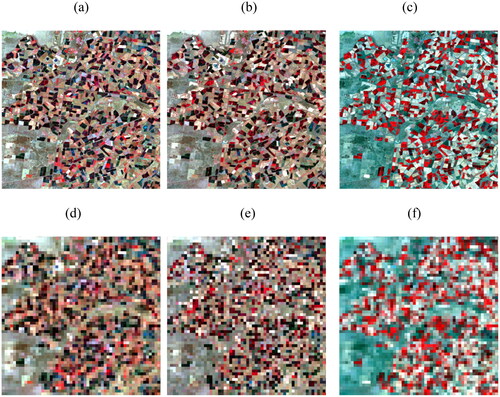
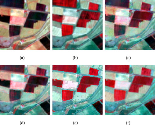
The first study area represents a heterogeneous landscape that is characterized by heterogeneity and complexity of land cover pattern. This area is located in southern New South Wales, Australia, and covers an area of 25.2 × 25.2 km² (840 × 840 pixels) with central coordinates of the area being 145.867°E and 34.910°S. The primary land uses in this area are cultivation and forestland. Three cloud-free Landsat ETM + images are used. Figure 2 shows the false-color composite (near infrared (NIR)-red-green) images of the study area, where the Landsat data were acquired on 25 November 2001 (Figure 2(a)), 3 December 2001 (Figure 2(b)) and 12 January 2002 (Figure 2(c)). Comparing Figure 2(a) and Figure 2(b) with Figure 2(c), it can be observed that the reflectance of the cultivated land area changed significantly. Because the local irrigation period is from October to November, the reflectance of the cultivated land is relatively low in Figure 2(a) and Figure 2(b). In contrast, the reflectance of the crops increased significantly in January (Figure 2 (c)). Therefore, we used a pair of images from 25 November 2001, to predict the Landsat images on 12 January 2002 (Figure 2(c)).

Figure 2. False-color composite images of a heterogeneous landscape: the Landsat images acquired on (a) 25 November 2001, 3 December 2001 and (c) 12 January 2002; (d), (c) and (d) are 450 m MODIS-like images aggregated from (a), (b) and (c).

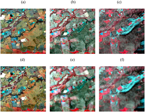
The second study area represents a landscape with land cover type change, located in northern New South Wales, Australia, covering an area of 25.2 × 25.2 km² (840 × 840 pixels). The central coordinates of the area are 149.056°E and 29.095°S. The landscape structure of this area is relatively simple, with cultivated land and woodland on both sides of the river (Figure 3(a) and Figure 3(b)). Landsat images of this area were acquired on 25 October 2004 (Figure 3(a)), 26 November 2004 (Figure 3(b)) and 12 December 2004 (Figure 3(c)). In December 2004, part of the area along the river was submerged (Figure 3(c)). Both phenological and land-cover type changes were observed in this study area from October to December. Therefore, in this experiment, we used a pair of images from 26 November 2004, to predict the Landsat images on 12 December 2004 (Figure 3(c)).

Figure 3. False-color composite images of a landscape with land cover type change: (a), (b) and (c) are Landsat images acquired on (a) 25 October 2004, (b) 26 November 2004 and (c) 12 December 2004; (c) and (d) are 450 m MODIS-like images aggregated from (a), (b) and (c).

4.2. Accuracy evaluation

The predicted images fused by the SE-STRFM are evaluated qualitatively and quantitatively using visual analysis and quantitative indices. The three models are visually and quantitatively compared with the actual images. The indices used to evaluate the accuracy include the root mean square error (RMSE), correlation coefficient (r), average absolute difference (AAD), and structure similarity index (SSIM) (Wang et al. 2004; Emelyanova et al. 2013). (24) $$\mathit{SSIM}=\frac{\left(2\overline{x}\overline{y}+C_1\right)\left(2{\sigma }_{XY}+C_2\right)}{\left({\overline{x}}^2+{\overline{y}}^2+C_1\right)\left({\sigma }_X+{\sigma }_Y+C_2\right)}$$(24) where $\overline{x}$ and $\overline{y}$ are the average reflectances in the fused and actual images, respectively; ${\delta }_X$ and ${\delta }_Y$ are the variances of the fused and actual images, respectively; ${\delta }_{XY}$ is the covariance of the two images; and $C_1$ and $C_2$ are two constants used to ensure stable results. For the RMSE and AAD, a smaller value indicates a better fusion effect; for r and SSIM, a value closer to 1 indicates a better fusion effect (Wang et al. 2004; Emelyanova et al. 2013).

Furthermore, the SE-STRFM is compared with the widely used fusion benchmark models STARFM (Gao et al. 2006), ESTARFM (Zhu et al. 2010) and FSDAF (Zhu et al. 2016). The predicted images fused by the three models are evaluated qualitatively and quantitatively using visual analysis and quantitative indices.

5. Results and analysis

5.1. Fusion results in the heterogeneous area

The fusion results of SE-STRFM and the other three models are shown in Figure 4. Compared to the actual image on the prediction date, the fusion results of the four models are visually similar (Figure 4(b–f)); however, SE-STRFM outperforms the other three models, as the spatial details and spectral information of the fusion image are closer to those of the actual image, as shown in the zoomed-in images (Figure 5(b–f)). Comparing to the actual image on the base and prediction dates, we found that the vegetation reflectance of several cultivated lands changed significantly in the zoomed-in area (Figure 5(a, b)). However, the fused image obtained using the STARFM and the ESTARFM did not predict this temporal change (Figure 5(c, d)). The vegetation reflectance of these cultivated lands in the fused image tended to be the same as that in the base image (Figure 5(a, c, d)). Although the FSDAF can accurately predict the change in vegetation reflectance for the small objects, the ‘plaque’ phenomenon is obvious in the fused result and the spatial details of the fused result are less significant than the ones in the actual image (Figure 5(e)). In comparison, the SE-STRFM is better for predicting temporal changes and preserving the spatial details of small objects (Figure 5(f)).

Figure 4. Actual images on the (a) base date and (b) predicted date, and the fusion images from (c) STARFM, (d) ESTARFM, (e) FSDAF, and (f) SE-STRFM.

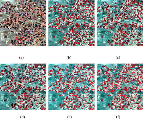
Figure 5. The zoomed-in images: actual images on the (a) base date and (b) predicted date, and the fusion images from (c) STARFM, (d) ESTARFM, (e) FSDAF, and (f) SE-STRFM.

The quantitative evaluation results for the fused images obtained using the three models are presented in Table 1. For all six bands, the fusion results of the SE-STRFM have the smallest RMSE and AAD, highest r, and highest SSIM, except for band 4. Comparing with the STARFM, the ESTARFM and the FSDAF, the RMSE of SE-STRFM is 16.74%, 17.97% and 6.81% lower on average, respectively; r is 6.02%, 5.77% and 1.61% higher on average, respectively; AAD is 14.82%, 16.76% and 6.98% lower on average, respectively; and SSIM is 5.97%, 5.77% and 1.80% higher on average, respectively.

Table 1. Accuracy assessment results for the test site with a heterogeneous landscape.

		Band1	Band2	Band3	Band4	Band5	Band7
RMSE	STARFM	0.0165	0.0234	0.0344	0.0509	0.0388	0.0301
	ESTARFM	0.0158	0.0224	0.0325	0.0545	0.0408	0.0310
	FSDAF	0.0147	0.0216	0.0322	0.0390	0.0373	0.0286
	SE-STRFM	0.0146	0.0208	0.0291	0.0378	0.0328	0.0265
r	STARFM	0.7833	0.8103	0.8615	0.7004	0.8983	0.9195
	ESTARFM	0.8000	0.8249	0.8750	0.6795	0.8909	0.9149
	FSDAF	0.8289	0.8393	0.8769	0.8152	0.9029	0.9257
	SE-STRFM	0.8328	0.8507	0.9004	0.8267	0.9254	0.9366
AAD	STARFM	0.0116	0.0162	0.0236	0.034	0.0271	0.0204
	ESTARFM	0.0112	0.0157	0.0226	0.0368	0.0286	0.0211
	FSDAF	0.0105	0.0154	0.0225	0.0268	0.0266	0.0199
	SE-STRFM	0.0104	0.0146	0.0202	0.0266	0.0232	0.0182
SSIM	STARFM	0.7788	0.7983	0.8492	0.704	0.9041	0.9223
	ESTARFM	0.7941	0.8111	0.8620	0.6839	0.8968	0.9178
	FSDAF	0.8202	0.8294	0.8699	0.8120	0.9028	0.9255
	SE-STRFM	0.8298	0.8466	0.8983	0.8103	0.9290	0.9384

The quantitative evaluations show that the SE-STRFM has a better performance than the benchmark methods (STARFM, ESTARFM and FSDAF). Specifically, the improvements in spectral accuracy (RMSE, AAD), and in structure similarity are significant compared with the STARFM, the ESTARFM and the FSDAF. On the other hand, the fused images by using the SE-STRFM have more spatial details, and its spectral information is closer to the actual image than that of the benchmark method (FSDAF) (Figure 5). This is because the SE-STRFM can predict pixel reflectance changes in sub-pixel level of fine-resolution images, while the FSDAF model predicts pixel reflectance change by assigning low-resolution endmember spectral reflectance changes to fine-resolution land cover types, which weakens spectral difference within the same land cover type area in the fusion image. Therefore, the FSADF model results in the loss of spatial details and more significant of plaque effect in fused image (Figure 5(e)).

5.2. Fusion results for land cover type changes

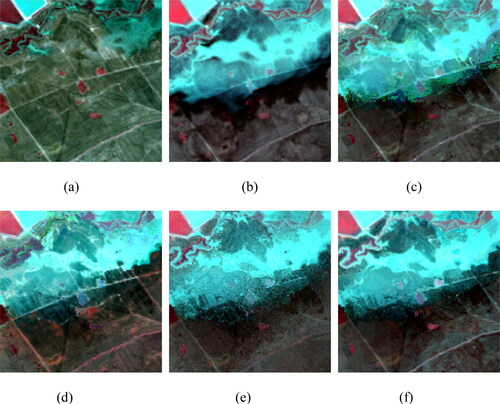
The fusion results for the SE-STRFM model are shown in Figure 6(f). Comparing with the STARFM, the ESTARFM and the FSDAF, the image predicted by the SE-STRFM is closer to the actual image in the zoomed-in images (Figure 7(b–f)). Comparing Figure 6(a, b), there are some land cover changes that are mostly caused by an increase in the water level. However, the STARFM and the ESTARFM can not effectively predict this sudden land cover change, and the spectral information of the predicted image is significantly different from that of the actual image (Figures 6(c, d) and 7(c, d)). Although the FSDAF could capture this land cover type change, its predicted image did not clearly show the boundary between the light and dark areas caused by flooding (Figures 6(e) and 7(e)). Therefore, the image predicted by FSDAF appears blurry. In contrast, the image predicted by SE-STRFM is closer to the actual image in terms of spectral information and spatial details (Figures 6(f) and 7 (f)). In addition, small patches of vegetation can still be clearly distinguished in the image predicted by the SE-STRFM, which are lost in the images predicted by the STARFM (Figures 6(c) and 7(c)), the ESTARFM (Figures 6(d) and 7(d)) and the FSDAF (Figures 6(e) and 7(e)).

Figure 6. Actual image on the (a) base date and (b) predicted date, and the fusion image of (c) STARFM, (d) ESTARFM, (e) FSDAF, and (f) SE-STRFM.

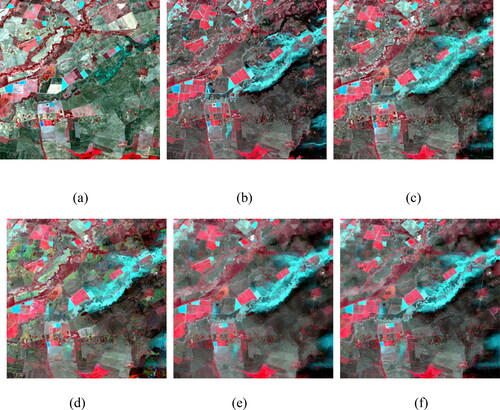
Figure 7. The zoomed-in images: actual image on the (a) base date and (b) predicted date, and the fusion image of (c) STARFM, (d) ESTARFM, (e) FSDAF, and (f) SE-STRFM.

The quantitative evaluation results show that, compared with the STARFM, the ESTARFM and the FSDAF, the image predicted by the SE-STRFM is closer to the actual image on the prediction date (Table 2). For all six bands, the fusion results obtained by the SE-STRFM have the smallest RMSE, and highest r and SSIM (except band 1). Compared with the STARFM, the ESTARFM and the FSDAF, the RMSE of the SE-STRFM is 4.29%, 33.81% and 6.35% lower on average, respectively; r is 1.32%, 14.88% and 1.69% higher on average, respectively; AAD is 3.28%, 32.39% and 7.60% lower on average, respectively; and SSIM is 0.35%, 14.54% and 2.03% higher on average, respectively.

Table 2. Accuracy assessment results for the test site with land cover type change.

		Band1	Band2	Band3	Band4	Band5	Band7
RMSE	STARFM	0.0136	0.0186	0.0213	0.0255	0.0422	0.0328
	ESTARFM	0.0140	0.0201	0.0252	0.0348	0.0715	0.0571
	FSDAF	0.0134	0.0178	0.0202	0.0253	0.0454	0.0353
	SE-STRFM	0.0130	0.0174	0.0197	0.0236	0.0418	0.0319
r	STARFM	0.8314	0.8285	0.8251	0.9182	0.8822	0.8810
	ESTARFM	0.8116	0.7893	0.7441	0.8477	0.6854	0.6784
	FSDAF	0.8308	0.8389	0.8371	0.9203	0.8613	0.8592
	SE-STRFM	0.8407	0.8465	0.8462	0.9298	0.8843	0.8871
AAD	STARFM	0.0097	0.0128	0.0144	0.0175	0.0290	0.0234
	ESTARFM	0.0097	0.0137	0.0172	0.0247	0.0475	0.0400
	FSDAF	0.0096	0.0123	0.0139	0.0180	0.0325	0.0255
	SE-STRFM	0.0092	0.0119	0.0132	0.0164	0.0295	0.0231
SSIM	STARFM	0.8315	0.8278	0.8253	0.9162	0.8752	0.8770
	ESTARFM	0.7984	0.7780	0.7401	0.8437	0.6786	0.6758
	FSDAF	0.8150	0.8224	0.8178	0.9139	0.8508	0.8484
	SE-STRFM	0.8270	0.8314	0.8280	0.9295	0.8759	0.8794

The accuracy indices (RMSE, r, AAD, SSIM) (Table 2) shows that the fused image using the FSDAF model is even worse than that of the STARFM in some bands. The SSIM of the FSDAF was lower than that of the STARFM in all image bands. The average changes of accuracy indicators of the SE-STRFM relative to the STARFM, the ESTARFM and the FSDAF are all high according to the above calculation results.

The fused image obtained using the SE-STRFM has more spatial details than that of the FSDAF, as shown in the zoomed-in images (Figure 7). On the other hand, the FSADF model allocated residuals caused by land cover changes using TPS interpolation, resulting in the fused image ‘smoothing’. Thus, the fused images obtained using the FSADF model loses many spatial details and causes image blurring (Figures 6 and 7).

6. Discussion

6.1. Reducing the impacts of heterogeneous landscapes

Among the existing spatial improved-type models in the STARFM-family, the well-known model is the Enhanced Spatial and Temporal Adaptive Reflectance Fusion Model (ESTARFM) proposed by Zhu et al. (2010) to improve the impacts of heterogeneous landscapes to some extent by adding input data pairs and introducing a conversion coefficient representing the reflectance change ratio. However, this model has not fundamentally solved the spatial details of the fused image, and the ‘plaque’ phenomenon of the fused image is relatively significant in heterogeneous landscapes.

Among the spatiotemporal improved-type models in the STARFM-family, a typical spatiotemporal improved-type model in the STARFM family is the Flexible Spatiotemporal Data Fusion (FSDAF) model proposed by Zhu et al. (2016), which predicts reflectance change caused by temporal and land-cover changes simultaneously. After that, a variety of improved FSDAF models have been rapidly developed based on various principles to further enhance its strength in capturing land-cover changes. Guo et al. (2020) proposed the FSDAF 2.0, incorporating change detection technology and an optimized model for changed areas to improve the FSDAF model to a certain extent. To produce a normalized difference vegetation index (NDVI) time series at a high spatiotemporal resolution, Liu et al. (2019) proposed the improved FSDAF (IFSDAF) model, which combines temporal and spatial predictions to produce an NDVI time series by adding input data pairs. These well-known spatiotemporal improved-type models in the STARFM family models (such as FSDAF, IFSDAF, and FSDAF2.0) estimate the abundance of endmembers at the land cover class level using hard-classification methods, and apply them in spatial-unmixing processes to downscale temporal changes for predicting temporal reflectance changes (Zhu et al. 2016; Guo et al. 2020; Li et al. 2020). As the endmember abundance calculated by a hard-classification map lacks intra-class variants, the predicted temporal changes in reflectance in the fusion images lose the intra-class variations, resulting in obvious ‘plaque’ phenomena and blurring in fused images.

To effectively predict the temporal reflectance change and land cover change simultaneously, Li et al. (2020) proposed an enhanced Flexible Spatiotemporal DAta Fusion (SFSDAF) model, which incorporates class fraction change information into spatiotemporal image fusion and enables superior predictions relative to existing methods. Hou et al. (2020) proposed an Adaptive-SFSDAF model by adaptively selecting fraction change to effectively improve the SFSDAF model. Recently, Shi et al. (2022) proposed the Reliable and Adaptive Spatiotemporal Data Fusion (RASDF) method to reduce the uncertainty of image fusion caused by sensor differences and retrieve strong temporal changes. Chen et al. (2022) proposed Variation-based Spatiotemporal Data Fusion (VSDF) model by considering systematically the temporal changes, introducing feature-level information, and exploiting the reliability of coarse images, which can capture abrupt land cover changes in heterogeneous areas and estimate the detailed spatial structure to some extent. The recently developed spatiotemporal improved-type models in the STARFM family models, such as SFSDAF and Adaptive-SFSDAF, have obtained endmember abundance by adopting soft classification (Li et al. 2020; Hou et al. 2020) to reduce intra-class variants to a certain extent. However, the soft classification still relies on the hard classification results, which causes calculated endmember abundance to lose intra-class variations to a certain extent, and the selection and number of endmembers based on clustering methods are affected by subjective influences from visual selection, which thus impacts the accuracy of the fused images (Rao et al. 2015).

To address the aforementioned limitations, the SE-STRFM enhances the spatial details of fused images by processing at the sub-pixel level of fine-resolution image. Comparing with the benchmark spatiotemporal fusion models such as the STARFM, the ESTARFM and the FSDAF, the SE-STRFM uses spectral unmixing theory to capture the temporal changes in spatial details and can predict fine-resolution images with more in-depth spatial details and more effectively address the ‘plaque’ phenomena and blurring in fused images than the benchmark models.

6.2. Predicting abrupt land cover changes

Some recently developed spatiotemporal improved-type models in the STARFM family models, such as the FSDAF, the IFSDAF, and the FSDAF2.0, can predict land cover change by estimating the residuals. Although the strategy of estimating land cover change is improved by the FSDAF and its variants, the assumption used in allocating the residuals by TPS is empirical and has no theoretical basis (Liu et al. 2019). Although the SFSDAF and the Adaptive-SFSDAF models utilize endmember abundance change information to estimate land cover changes, relatively complex computation with some assumptions lead to uncertainties and a large computational burden for the prediction process. With further development of the FSDAF variant models, the models tend to be more complex, leading to difficulties in their implementation, especially in large areas (Chen et al. 2023). The relatively long computation chain with some assumptions in each step, wherein errors generated by the entire computation chain cannot be ignored, not only leads to a large computational burden but introduces uncertainties in the prediction model. The SE-STRFM predicts land cover changes using a simple interpretation method and weighting function. Compared with existing the STARFM family models can accurately predict land cover change and preserve the spatial details of small objects more effectively. Specifically, the fused image obtained using the SE-STRFM has more spatial details than that of the FSDAF. This is because the FSDA results in the fused image ‘smoothing’ using TPS interpolation to allocate residuals.

6.3. Limintation and future work

Although the proposed SE-STRFM can accurately predict temporal changes and rapid land cover changes, adaptive spatial unmixing analysis for spectral component inversion and multi-temporal spectral unmixing analysis (Liu et al. 2016) will be investigated further in the future to improve the fusion efficiency.

The proposed model was tested in two typical areas where the previous studies have been widely used. However, these two study areas are flat. In order to confirm that the proposed model has the same accuracy in rugged terrains as well as flat areas, we will conduct further validation in rugged terrains in subsequent model applications. For rugged terrain areas, the terrain shadow is a main impact influence factor. The vegetation or soil in terrain shadow areas can be represented by low albedo endmember during linear spectral unmixing process. Theoretically, the proposed model is applicable for complex topographic areas. The further experimental verification is needed. In the experiment, we only evaluated and compared the three benchmark spatiotemporal data fusion models, which would not serve as favorable evidence that the SE-STRFM is superior to other latest models. In future research, we will validate and compare with the latest fusion models to further analyze the performance of the SE-STRFM.

7. Conclusions

The current STARFM family models face the issues of missing spatial details and the plaque effect in fused images. We proposed the Spatial Enhanced Spatiotemporal Reflectance Fusion Model (SE-STRFM) to predict fine-resolution images on the sub-pixel scale using spectral unmixing theory to capture the temporal changes in spatial details and rapid land-cover type changes. The SE-STRFM effectively eliminate the obvious ‘plaque’ phenomenon and image blurring in fused images. In addition, the SE-STRFM only requires one pair of fine- and coarse-resolution images as the base data and one coarse image for prediction.

The SE-STRFM model employs a spectral unmixing method to obtain the endmember abundance of fine-resolution pixels and aggregates to determine the endmember abundance of coarse-resolution pixels. Then, the temporal change in each endmember’s reflectance is estimated and assigned to the fine-resolution abundance pixel by pixel. Afterwards, the residuals of reflectance caused by land cover change are calculated at a coarse resolution and downscaled to a fine resolution by resampling and weighting functions with similar pixel selection. Finally, the prediction image is obtained by adding the predicted reflectance change and residuals of the fine-resolution image to the reflectance of the base fine-resolution image. To verify the applicability of the framework, we chose two typical study areas that have been used in previous studies and performed qualitative and quantitative accuracy evaluations. The results show that the images fused by the SE-STRFM have clearer spatial details and a more accurate spectral distribution compared with those fused by the STARFM, the ESTARFM and the FSDAF.

Acknowledgements

The authors would like to thank the editors and anonymous reviewers for the valuable comments, which helped improve this paper.

Disclosure statement

No potential conflict of interest was reported by the author(s).

Additional information

Funding

This work was supported by the National Natural Science Foundation of China [No. 42171364; No. 42171452].

Notes

1 •••

References

- Cai J, Huang B, Fung T. 2022. Progressive spatiotemporal image fusion with deep neural networks. Int J Appl Earth Obs Geoinf. 108:102745. doi: 10.1016/j.jag.2022.102745.
- Chen B, Huang B, Xu B. 2017. Multi-source remotely sensed data fusion for improving land cover classification. ISPRS J Photogramm Remote Sens. 124:27–39. doi: 10.1016/j.isprsjprs.2016.12.008.
- Chen S, Wang J, Gong P. 2023. ROBOT: a spatiotemporal fusion model toward seamless data cube for global remote sensing applications. Remote Sens Environ. 294:113616. doi: 10.1016/j.rse.2023.113616.
- Chen X, Du X, Yan Z, Zhu J, Xu S, Fan X. 2022. VSDF: a variation-based spatiotemporal data fusion method. Remote Sens Environ. 283:113309. doi: 10.1016/j.rse.2022.113309.
- Emelyanova I, McVicar T, Van Niel T, Li L, M, van Dijk A. 2013. Assessing the accuracy of blending Landsat–MODIS surface reflectances in two landscapes with contrasting spatial and temporal dynamics: a framework for algorithm selection. Remote Sens Environ. 133:193–209. doi: 10.1016/j.rse.2013.02.007.
- Fu D, Chen B, Wang J, Zhu X, Hilker T. 2013. An improved image fusion approach based on enhanced spatial and temporal the adaptive reflectance fusion model. Remote Sens. 5(12):6346–6360. doi: 10.3390/rs5126346.
- Gao F, Masek J, Schwaller M, Hall F. 2006. On the blending of the Landsat and MODIS surface reflectance: predicting daily Landsat surface reflectance. IEEE Trans. Geosci. Remote Sens, 44(12):2207–2218. doi: 10.1109/TGRS.2006.872081.
- Gao F, Anderson MC, Zhang X, Yang Z, Alfieri JG, Kustas WP, Mueller R, Johnson DM, Prueger JH. 2017. Toward mapping crop progress at field scales through fusion of Landsat and MODIS imagery. Remote Sens Environ. 188:9–25. doi: 10.1016/j.rse.2016.11.004.
- Gao H, Zhu X, Guan Q, Yang X, Yao Y, Zeng W, Peng X. 2022. cuFSDAF: an Enhanced Flexible Spatiotemporal Data Fusion Algorithm Parallelized Using Graphics Processing Units. IEEE Trans Geosci Remote Sens. 60:1–16. doi: 10.1109/TGRS.2021.3080384.
- Gong P, Wang J, Yu L, Zhao YC, Zhao YY, Liang L, Niu Z, Huang X, Fu H, Liu S, et al. 2013. Finer resolution observation and monitoring of global land cover: first mapping results with landsat TM and ETM + data. Int J Remote Sens. 34(7):2607–2654. doi: 10.1080/01431161.2012.748992.
- Gong P, Li X, Wang J, Bai Y, Chen B, Hu T, Liu X, Xu B, Yang J, Zhang W, et al. 2020. Annual maps of global artificial impervious area (GAIA) between 1985 and 2018. Remote Sens. Environ. 236:111510. doi: 10.1016/j.rse.2019.111510.
- Gevaert CM, García-Haro FJ. 2015. A comparison of STARFM and an unmixing-based algorithm for Landsat and MODIS data fusion. Remote Sens Environ. 156:34–44. doi: 10.1016/j.rse.2014.09.012.
- Ghosh R, Gupta PK, Tolpekin V, Srivastav SK. 2020. An enhanced spatiotemporal fusion method – implications for coal fire monitoring using satellite imagery. Int J Appl Earth Obs Geoinf. 88:102056. doi: 10.1016/j.jag.2020.102056.
- Guo D, Shi W, Hao M, Zhu X. 2020. FSDAF 2.0: improving the performance of retrieving land cover changes and preserving spatial details. Remote Sens Environ. 248:111973. doi: 10.1016/j.rse.2020.111973.
- Hilker T, Wulder MA, Coops NC, Linke J, McDermid G, Masek JG, Gao F, White JC. 2009. A new data fusion model for high spatial- and temporal-resolution mapping of forest disturbance based on Landsat and MODIS. Remote Sens Environ. 113(8):1613–1627. doi: 10.1016/j.rse.2009.03.007.
- Hou S, Sun W, Guo B, Li C, Li X, Shao Y, Zhang J. 2020. Adaptive-SFSDAF for spatiotemporal image fusion that selectively uses class abundance change information. Remote Sens. 12(23):3979. doi: 10.3390/rs12233979.
- Huang B, Song H. 2012. Spatiotemporal Reflectance Fusion via Sparse Representation. IEEE Trans Geosci Remote Sens. 50(10):3707–3716. doi: 10.1109/TGRS.2012.2186638.
- Jafarzadeh H, Hasanlou M. 2019. An Unsupervised Binary and Multiple Change Detection Approach for Hyperspectral Imagery Based on Spectral Unmixing. IEEE J Sel Top Appl Earth Observat Remote Sens. 12(12):4888–4906. doi: 10.1109/JSTARS.2019.2939133.
- Ju J, Roy DP. 2008. The availability of cloud-free Landsat ETM + data over the conterminous United States and globally. Remote Sens Environ. 112(3):1196–1211. doi: 10.1016/j.rse.2007.08.011.
- Kong F, Li X, Wang H, Xie D, Li X, Bai Y. 2016. Land Cover Classification Based on Fused Data from GF-1 and MODIS NDVI Time Series. Remote Sens. 8(9):741. doi: 10.3390/rs8090741.
- Li A, Bo Y, Zhu Y, Guo P, Bi J, He Y. 2013. Blending multi-resolution satellite sea surface temperature (SST) products using Bayesian maximum entropy method. Remote Sens Environ. 135:52–63. doi: 10.1016/j.rse.2013.03.021.
- Li Y, Huang C, Hou J, Gu J, Zhu G, Li X. 2017. Mapping daily evapotranspiration based on spatiotemporal fusion of ASTER and MODIS images over irrigated agricultural areas in the Heihe River Basin, Northwest China. Agric For Meteorol. 244–245:82–97. doi: 10.1016/j.agrformet.2017.05.023.
- Li X, Foody GM, Boyd DS, Ge Y, Zhang Y, Du Y, Ling F. 2020. SFSDAF: an enhanced FSDAF that incorporates sub-pixel class fraction change information for spatio-temporal image fusion. Remote Sens Environ. 237:111537. doi: 10.1016/j.rse.2019.111537.
- Liao L, Song J, Wang J, Xiao Z, Wang J. 2016. Bayesian method for building frequent landsat-like NDVI datasets by integrating MODIS and Landsat NDVI. Remote Sens. 8(6):452. doi: 10.3390/rs8060452.
- Liu S, Bruzzone L, Bovolo F, Du P. 2016. Unsupervised multitemporal spectral unmixing for detecting multiple changes in hyperspectral images. IEEE Trans Geosci Remote Sens. 54(5):2733–2748. doi: 10.1109/TGRS.2015.2505183.
- Liu M, Yang W, Zhu X, Chen J, Chen X, Yang L, Helmer EH. 2019. An Improved Flexible Spatiotemporal Data Fusion (IFSDAF) method for producing high spatiotemporal resolution normalized difference vegetation index time series. Remote Sens Environ. 227:74–89. doi: 10.1016/j.rse.2019.03.012.
- Liu W, Zeng Y, Li S, Huang W. 2020. Spectral unmixing based spatiotemporal downscaling fusion approach. Int J Appl Earth Obs Geoinf. 88:102054. doi: 10.1016/j.jag.2020.102054.
- Liu W, Zeng Y, Li S, Pi X, Huang W. 2019. An improved spatiotemporal fusion approach based on multiple endmember spectral mixture analysis. Sensors. 19(11):2443. doi: 10.3390/s19112443.
- Lu D, Batistella M, Moran E. 2004. Multitemporal spectral mixture analysis for Amazonian land-cover change detection. Can J Remote Sens. 30(1):87–100. doi: 10.5589/m03-055.
- Mariana B, Alfred S. 2019. Spatiotemporal image fusion in remote sensing. Remote Sens. 11:818.
- Moosavi V, Talebi A, Mokhtari MH, Shamsi SRF, Niazi Y. 2015. A wavelet-artificial intelligence fusion approach (WAIFA) for blending Landsat and MODIS surface temperature. Remote Sens Environ. 169:243–254. doi: 10.1016/j.rse.2015.08.015.
- Peng K, Wang Q, Tang Y, Tong X, Atkinson PM. 2022. Geographically weighted spatial unmixing for spatiotemporal fusion. IEEE Trans Geosci Remote Sens. 60:1–17. doi: 10.1109/TGRS.2021.3115136.
- Rao Y, Zhu X, Chen J, Wang J. 2015. An improved method for producing high spatial-resolution NDVI Time series datasets with multi-temporal MODIS NDVI data and Landsat TM/ETM + images. Remote Sens. 7(6):7865–7891. doi: 10.3390/rs70607865.
- Ridd M. 1995. Exploring a V–I–S (vegetation–impervious–surface-soil) model for urban ecosystem analysis through remote sensing: comparative anatomy for cities. Int J Remote Sens. 16(12):2165–2185. doi: 10.1080/01431169508954549.
- Semmens K, Anderson M, Kustas W, Gao F, Alfieri J, McKee L, Prueger J, Hain C, Cammalleri C, Yang Y, et al. 2016. Monitoring daily evapotranspiration over two California vineyards using Landsat 8 in a multi-sensor data fusion approach. Remote Sens Environ. 185:155–170. doi: 10.1016/j.rse.2015.10.025.
- Shi W, Guo D, Zhang H. 2022. A reliable and adaptive spatiotemporal data fusion method for blending multi-spatiotemporal-resolution satellite images. Remote Sens Environ. 268:112770. doi: 10.1016/j.rse.2021.112770.
- Somers B, Asner G, Tits L, Coppin P. 2011. Endmember variability in spectral mixture analysis: a review. Remote Sens Environ. 115(7):1603–1616. doi: 10.1016/j.rse.2011.03.003.
- Small C. 2003. High spatial resolution spectral mixture analysis of urban reflectance. Remote Sens Environ. 88(1-2):170–186. doi: 10.1016/j.rse.2003.04.008.
- Small C. 2004. The Landsat ETM + spectral mixing space. Remote Sens Environ. 93(1–2):1–17. doi: 10.1016/j.rse.2004.06.007.
- Singh D. 2011. Generation and evaluation of gross primary productivity using Landsat data through blending with MODIS data. Int J Appl Earth Obs Geoinf. 13(1):59–69. doi: 10.1016/j.jag.2010.06.007.
- Tran T, De Beurs K, Julian J. 2016. Monitoring forest disturbances in Southeast Oklahoma using Landsat and MODIS images. Int J Appl Earth Obs Geoinf. 44:42–52. doi: 10.1016/j.jag.2015.07.001.
- Wang Q, Ding X, Tong X, Atkinson P. 2021. Spatio-temporal spectral unmixing of time-series images. Remote Sens Environ. 259:112407. doi: 10.1016/j.rse.2021.112407.
- Wang X, Jia K, Liang S, Li Q, Wei X, Yao Y, Zhang X, Tu Y. 2017. Estimating fractional vegetation cover from landsat-7 ETM + reflectance data based on a coupled radiative transfer and crop growth model. IEEE Trans Geosci Remote Sensing. 55(10):5539–5546. doi: 10.1109/TGRS.2017.2709803.
- Wang Z, Bovik A, Sheikh H, Simoncelli E. 2004. Image quality assessment: from error visibility to structural similarity. IEEE Trans Image Process. 13(4):600–612. doi: 10.1109/tip.2003.819861.
- Watts JD, Powell SL, Lawrence RL, Hilker T. 2011. Improved classification of conservation tillage adoption using high temporal and synthetic satellite imagery. Remote Sens Environ. 115(1):66–75. doi: 10.1016/j.rse.2010.08.005.
- Weng Q, Fu P, Gao F. 2014. Generating daily land surface temperature at Landsat resolution by fusing Landsat and MODIS data. Remote Sens Environ. 145:55–67. doi: 10.1016/j.rse.2014.02.003.
- Wu B, Huang B, Zhang L. 2015. An error-bound-regularized sparse coding for spatiotemporal reflectance fusion. IEEE Trans Geosci Remote Sensing. 53(12):6791–6803. doi: 10.1109/TGRS.2015.2448100.
- Wu C, Murray AT. 2003. Estimating impervious surface distribution by spectral mixture analysis. Remote Sens Environ. 84(4):493–505. doi: 10.1016/S0034-4257(02)00136-0.
- Wu M, Niu Z, Wang C, Wu C, Wang L. 2012. Use of MODIS and Landsat time series data to generate high-resolution temporal synthetic Landsat data using a spatial and temporal reflectance fusion model. J Appl Rem Sens. 6(01):1–14. doi: 10.1117/1.JRS.6.063507.
- Wu M, Huang W, Niu Z, Wang C, Li W, Yu B. 2018. Validation of synthetic daily Landsat NDVI time series data generated by the improved spatial and temporal data fusion approach. Inf Fusion. 40:34–44. doi: 10.1016/j.inffus.2017.06.005.
- Yang Y, Anderson M, Gao F, Hain C, Noormets A, Sun G, Wynne R, Thomas V, Sun L. 2020. Investigating impacts of drought and disturbance on evapotranspiration over a forested landscape in North Carolina, USA using high spatiotemporal resolution remotely sensed data. Remote Sens Environ. 238:111018. doi: 10.1016/j.rse.2018.12.017.
- Zhang B, Zhang L, Xie D, Yin X, Liu C, Liu G. 2016. Application of Synthetic NDVI Time Series Blended from Landsat and MODIS Data for Grassland Biomass Estimation. Remote Sens. 8(1):10. doi: 10.3390/rs8010010.
- Zhang F, Zhu X, Liu D. 2014. Blending MODIS and Landsat images for urban flood mapping. Int J Remote Sens. 35(9):3237–3253. doi: 10.1080/01431161.2014.903351.
- Zhang H, Huang B, Zhang M, Cao K, Yu L. 2015. A generalization of spatial and temporal fusion methods for remotely sensed surface parameters. Int J Remote Sens. 36(17):4411–4445. doi: 10.1080/01431161.2015.1083633.
- Zhu X, Chen J, Gao F, Chen X, Masek JG. 2010. An enhanced spatial and temporal adaptive reflectance fusion model for complex heterogeneous regions. Remote Sens Environ. 114(11):2610–2623. doi: 10.1016/j.rse.2010.05.032.
- Zhu X, Helmer EH, Gao F, Liu D, Chen J, Lefsky MA. 2016. A flexible spatiotemporal method for fusing satellite images with different resolutions. Remote Sens Environ. 172:165–177. doi: 10.1016/j.rse.2015.11.016.
- Zhu X, Cai F, Tian J, Williams TK-A. 2018. Spatiotemporal fusion of multisource remote sensing data: literature survey, taxonomy, principles, applications, and future directions. Remote Sens. 10(4):527. doi: 10.3390/rs10040527.
- Zhukov B, Oertel D, Lanzl F, Reinhackel G. 1999. Unmixing-based multisensor multiresolution image fusion. IEEE Trans Geosci Remote Sens. 37(3):1212–1226. doi: 10.1109/36.763276.