Blue-green water resource availability dynamics in the upper Awash basin, central Ethiopia: implications for agricultural water scarcity assessment

Abstract

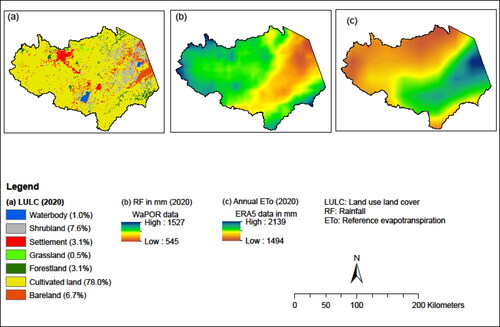
Quantifying and characterizing the spatial distribution of freshwater availability and water scarcity plays an indispensable role in managing water resources in a basin. This study aimed at quantifying green and blue water resource availability using an eco-hydrological model under different land use land cover conditions between 2000–2010 and 2020 in the upper Awash basin, central Ethiopia. Further, the agricultural water scarcity is assessed for dominantly cultivated crops in the basin. The freshwater components such as the green water (GW) flow (∼1041–1240 mm/yr), blue water (BW) flow (277–304 mm/yr), and GW storage (809-872 mm/yr) were observed to be high in the western highlands compared to the central and eastern parts of the basin. The results of GW scarcity indices show low to moderate scarcity for rainfed crops, and moderate to significant BW scarcity for irrigated sugarcane. Integrating GW potential to reduce BW scarcity in the basin is thus crucial.

Keywords:

• Green water flow/storage
• blue water flow
• water availability
• green/blue water scarcity
• upper Awash basin

1. Introduction

Freshwater availability is an important ecosystem service that plays a significant role in supporting the sustainable development goals (SDGs), such as SDG 2: ending hunger; SDG 6: sustainable water use (particularly SDG 6.6.1 water-related ecosystem); SDG 11: sustainable cities and communities; and SDG 15: protecting, restoring, and promoting the sustainable use of ecosystems (life on land) (Hoekstra et al. 2017; Báldi and Vári 2020; Libala et al. 2022). Though water resources are abundant in Africa, the spatiotemporal variability among and within countries and river basins exacerbates water shortage problems (UN-Water/Africa 2006; Schuol et al. 2008).

According to Falkenmark and Rockström (2006), Schuol et al. (2008) and Zhang et al. (2019), freshwater components are categorized as green water flow (GWF; actual evapotranspiration), blue water flow (BWF; water yield including deep aquifer recharge), and green water resources or storage (GWS; soil water). In Sub-Saharan African (SSA) countries, 95% of the available green water is used by rainfed agriculture to support plant growth (Rockström et al. 2007), while blue water is used for domestic, irrigation, and industrial consumption (Quinteiro et al. 2018). Water trade-offs for various purposes, such as irrigating lands, domestic uses, and supporting the ecosystem, are increasing and significantly affecting blue water availability worldwide (Falkenmark and Rockström 2006).

Various studies have attempted to quantify blue-green water availability worldwide. Lee and Bae (2015) investigated the climate change influence on future blue and green water availability in the Asian Monsson region using the Variable Infiltration Capacity (VIC) hydrologic model. Xu et al. (2023) studied the dynamics of GWF in relation to climate and land use/land cover changes using ESSI-3 (the third version of the infiltration excess and Saturation excess Soil-water Integration) for the Sanjiang plain in China. In addition, the blue and green water resource of Poyang lake basin (Liu et al. 2023) and Iranian watershed (Sayyad et al. 2015) were examined using the Soil and Water Assessment Tool (SWAT). Du et al. (2018) studied the historical trends of water availability (in terms of green and blue water) in the Ohio River Basin in the U.S.A., whereas Li et al. (2022) assessed the green and blue water for large-scale watersheds of Southwest China using the MIKE SHE HYDRO model. The Water Availability and Adaptation Policy Assessment (WAAPA) model was also used to quantify the future blue water availability in Europe (Sordo-Ward et al. 2019). However, freshwater investigations using the green and blue water concepts in Africa are rare, except those of Rockström et al. (2007) and Schuol et al. (2008) whose studies considered 95 developing countries in the world including SSA countries, and the entire Africa, respectively. Furthermore, Serur (2020) modeled green and blue water resources for the Weyb River basin in Ethiopia. These studies show that the classical assessment of blue water availability, ignoring green water resources, underestimates the available water resources within the continents, countries, or basins or watersheds, particularly for rain-dependent SSA countries that heavily rely on green water (Rockström et al. 2007; Schuol et al. 2008; Li et al. 2022). In addition, basin-scale water availability is significantly influenced by sectoral water demands, climate change impacts and anthropogenic factors on land use changes, all of which lead to water scarcity (Swain et al. 2020; Liu et al. 2022). Thus, investigation of freshwater availability in different watersheds, and land use land cover (LULC) conditions combined with analysis of agricultural water scarcity for rainfed and irrigated crops is vital for effective green and blue water resource planning and management in water-scarce basins such as the upper Awash basin, in central Ethiopia.

Over the past few decades, the Awash basin has experienced a surge in water demand attributed to the expansion of agricultural practices, population growth in major cities such as Addis Ababa and Adama, and the establishment of industrial zones (Daba and You 2022). These factors have been worsening the problems related to availability of freshwater in the upper Awash basin along with climate change impacts, inefficient water management practices including outdated irrigation techniques and inefficient water distribution systems. For instance, the entire Awash basin experienced a freshwater deficit of 0.03 billion m³ annually compared to the average surface water demand (Adeba et al. 2015). Moreover, large-scale irrigation schemes have led to waterlogging and salinization exacerbating the problems related to quality and quantity of freshwater (Asad et al. 2018). Many studies in the Awash River basin have investigated the impacts of LULC on runoff, sediment yield, stream flow, peak discharge, and sedimentation using different hydrological models (e.g. Adane et al. 2021; Gemechu 2014; Shawul and Chakma 2018; Shawul et al. 2019). However, none of them attempted to quantify the spatio-temporal changes in blue and green water resources in the basin. Our study uses the Integrated Valuation of Ecosystem Service and Tradeoffs (InVEST) model to characterize various types of freshwater components and their temporal dynamics, including GWF at basin and watershed levels and under different LULC conditions, using Budyko curves (Sharp et al. 2014). The INVEST model has been tested to quantify the water yield in various parts of the world using GIS and Remote Sensing techniques for hydrologic modeling, including in South America (Goldman et al. 2010; Benra et al. 2021), North America (Scordo et al. 2018), Asia (Wei et al. 2021; Bejagam et al. 2022; Halder et al. 2022; Wang et al. 2022), and eastern Africa (Belete et al. 2018; Aneseyee et al. 2022). InVEST has an advantage over other hydrologic models including: (i) its simplified representation of hydrological processes, (ii) it can be easily integrated with ArcGIS, and (iii) it can quantify and map the spatial water yield and ecosystem services in a watershed with limited input data (Canqiang et al. 2012; Lüke and Hack 2018). Our study follows a new approach that was not tried before in the SSA countries, as it integrates the spatial water resource availability in different LULCs with green-blue water footprints (WFs) of dominantly cultivated crops in the upper Awash basin, which helps to understand the agricultural water scarcity conditions.

This study aims to particularly assess spatio-temporal dynamics of green and blue water resources by quantifying GWF, GWS, and BWF considering decadal LULC change and climatic conditions in the upper Awash basin. This study further provides insight into the availability of green water resources, which has been neglected as a potential water resource by researchers and policymakers in Africa because more attention has been given only to blue water resource management. In our previous studies, we estimated the green and blue water footprints in the upper Awash basin (Hirpa et al. 2022). The severity of the basin’s agricultural water scarcity has also been investigated using the water footprint framework and the modelled water resource availability. The results of this study will assist water managers and policymakers in setting benchmarks on the natural water flows and to assess the contribution of the agricultural sector in causing blue water scarcity in the basin .

2. Methodology

2.1. Study area

The upper Awash basin comprises highland and rift watersheds, which are characterized by an extensive rugged plateau reaching up to 4177 m above sea level (a.s.l.) to the west, on the highlands, and ∼794 m a.s.l. to the east, within the Main Ethiopian Rift (MER) (Hirpa et al. 2023). The total area of the upper Awash basin is ∼23,761 km² and it consists of nine watersheds: Akaki, Melka Kuntire, Holleta, Hombole, Mojo, Koka, Sire, Metehara and Kessem (Figure 1). The Melka Kuntire, Holleta, Akaki and Hombole are on the highlands of the western part of the basin, while Sire watershed underlies the southeastern highlands of the basin. Mojo and Koka watersheds are within the central part of the MER, while Kesem and Metehara are in the eastern part of the basin within the MER.

Figure 1. Location map of the upper Awash basin and its watersheds.

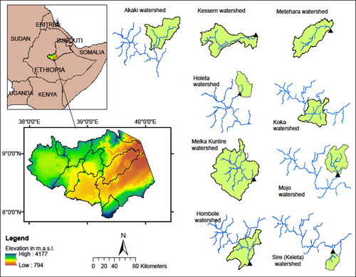
The average annual temperature decreases from the east (25 °C at Metehara) to the western part of the basin (8.6 °C at Mount Dendi). Evapotranspiration shows similar decreasing trend from the eastern to the western part of the basin (Figure 1). The basin is characterized by two distinct rainy seasons, with average annual rainfall of 985 mm (upstream of Koka reservoir) and 610 mm in the semi-arid area near Metehara (Adane et al. 2020b; Hirpa et al. 2022). The highlands are densely populated and dominated by intensive subsistence farming, and floriculture with some natural forests. On the other hand, large-scale irrigation schemes on the relatively flat topography dominate the MER where the Awash River and groundwater boreholes are the major sources of water to meet the consumptive water use of the irrigated crops.

2.2. Data and software

In this study, the free and open source InVEST version 3.11.0 software was used for quantitative evaluation of water yield. Input parameters (data) for this study include rainfall, reference evapotranspiration, LULC, soil properties, shape files of the basin and its watersheds (including Digital elevation Model – DEM), biophysical attribute of different LULC, and seasonality factor (Z) (Sharp et al. 2014). In addition, ArcMaP 10.6 software was used to organize the LULC maps, delineation of the nine watersheds and the basin, and interpret the output of InVEST software.

The input data for the InVEST model are arranged in a raster format and produce an explicit output that can be interpreted using the ArcMap software. All raster data were resampled at a spatial resolution of 30 m and projected using the World Geodetic System 84 (WGS84). From our previous studies (Hirpa et al. 2022), the green and blue water footprints of various irrigated sugarcane (with 24-, 20- and14-months length of growing period) and rainfed crops (Teff, maize and sorghum) were used for the analysis of the agricultural (green/blue) water scarcity. The input data, data type/resolution, and sources used to compute the blue-green water flows using the InVEST model, as well as the agricultural water scarcity indices are given in Table 1.

Table 1. Input data type and sources for blue and green water flow (GWF) estimation using the InVEST model and agricultural water scarcity indices.

Data input	Resolution/Time	Data source/Remark
Observed rainfall and temperature	Daily and annual (2000-2010)	National Meteorological Agency (NMA)
Satellite rainfall	Annual, Raster format (.tif), 0.05º, 2020	WaPOR database https://wapor.apps.fao.org/home/WAPOR_2/1 and https://aquastat.fao.org/climate-information-tool/complete-climate-data
Digital Elevation Model (DEM)	30 m × 30 m	Shuttle Radar Topographic Mission (SRTM) https://earthexplorer.usgs.gov/
Observed stream flow	Monthly and annual (2000-2010)	Ministry of Water and Energy of Ethiopia
Gridded evapotranspiration (ERA-5)	Annual, raster format (.tif), 0.25º (2000-2010 and 2020)	ECMWF's Copernicus Climate Change Service product (https://app.climateengine.com/climateEngine).
Soil depth and root depth	Raster format (.tif)	Adane et al. (2021), Harmonized World Soil Database (HWSD) (https://www.fao.org/soils-portal/data-hub/soil-maps-and-databases)
Plant Available Water Content (PAWC)	Raster format (.tif)	Adane et al. (2021), HWSD document, and Soil-Plant-Air-Water (SPAW) software
Land use land cover (LULC)	Raster format (.tif) (2000, 2010 and 2020)	Hirpa et al. 2023
Biophysical attribute	Microsoft Excel in .csv format	Adane et al. (2021), Allen et al. (1998) and other literature
Basin and watersheds	Shapefiles (.shp)	Delineated using ArcSWAT
Green and blue water footprints for maize, sorghum, and sugarcane	Decadal average (2000-2010)	Hirpa et al. (2022)

2.3. Methods

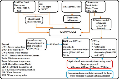
The InVEST model is a process-based ecosystem model that embeds hydrological and other tools for decision support in natural resource management (Sharp et al. 2014). It is a spatially explicit and lumped model that uses various physical and climatic parameters to quantify spatial water yield in a given basin (Sharp et al. 2014; Kusratmoko and Semedi 2019). This model has a comparative advantage in providing an effective means to estimate ecosystem services, such as water yield (i.e. BWF), at high spatial resolution using Budyko’s framework approaches and annual rainfall (Vigerstol and Aukema 2011; Dennedy-Frank et al. 2016). However, the model cannot provide an uncertainty estimation of the water yield based on past and future drivers of change (Yin et al. 2020). Furthermore, the BWF estimation in the InVEST model includes soil water content, water-holding capacity, and surface runoff (Yang et al. 2019). For this study, this simple water balance model was used to quantify the green-blue water resources in the upper Awash basin. The methodological framework for computation of green-blue water resources and agricultural water scarcity assessment is summarized in Figure 2.

Figure 2. Methodological framework for computation of green-blue water resources in the upper Awash basin.

2.3.1. Land use land cover (LULC)

In this study, decadal LULC maps (2000, 2010 and 2020) which were developed from our previous study is used as input in the InVEST model. The detailed methodological approaches and developed maps on LULC at the basin and watershed levels are reported in Hirpa et al. (2023).

2.3.2. Rainfall (P) and reference evapotranspiration (ETo)

Daily rainfall and temperature data for the period 2000–2010 from 22 stations in the upper Awash basin were obtained from the National Meteorological Services Agency of Ethiopia. The spatial map of annual rainfall and the ETo were produced using an Inverse Distance Weighting (IDW) interpolation method in the ArcGIS spatial analyst tool. ETo was calculated using the temperature-based Hargreaves equation (Hargreaves and Samani 1985; Hargreaves and Allen 2003) as indicated in Equation (1)(1) $$E{T}_o=C{R}_a{\left(T_{\max }-T_{\min }\right)}^E\left[\frac{T_{\max }+T_{\min }}{2}+T\right]$$(1) . (1) $$E{T}_o=C{R}_a{\left(T_{\max }-T_{\min }\right)}^E\left[\frac{T_{\max }+T_{\min }}{2}+T\right]$$(1) where T_max and T_min are the mean daily maximum and minimum temperatures in °C, respectively; Ra is the extra-terrestrials radiation based on latitudinal and other data inputs in mm d⁻¹ or J m⁻²S⁻¹, and C, E, and T are empirical parameters (0.0023, 0.5 and 17.8, respectively).

Subsequently, the spatial ETo map computed using the observed data was compared with ERA5 (the fifth generation European Centre for Medium-Range Weather Forecasts (ECMWF) atmospheric reanalysis of the global climate) gridded evapotranspiration output (https://app.climateengine.com/climateEngine). The meteorological stations in the eastern part of the basin are sparsely distributed, and the observed temperature records have consecutive missing years. Unlike the eastern part of the basin, the results in the western and central highlands were comparable. Thus, to capture the reference evapotranspiration of the entire catchment, we used ERA-5 gridded data as input to determine the green and blue water resource availability from 2000–2010 and 2020.

2.3.3. Plant available water content (PAWC) and soil depth

PAWC is the difference between the fraction of volumetric field capacity and wilting point. This parameter can be estimated based on the physical and chemical properties of soil (Rab et al. 2011). The Harmonized World Soil Database was used to obtain the soil’s physical characteristics in the basin, including its composition in terms of sand, silt and clay as well as its reference depth (https://www.fao.org/soils-portal/data-hub/soil-maps-and-databases). In addition, our previous findings (Adane et al. 2021) and the Soil-Plant-Atmosphere-Water (SPAW) software were used to generate the PAWC and process it in ArcGIS to prepare the spatial map. Thus, the spatial data were arranged to a fraction from 0 to 1 as required by the model input specifications (Jafarzadeh et al. 2021).

2.3.4. Watersheds delineation and biophysical properties

The Shuttle Radar Topographic Mission (SRTM) DEM data with 30 m resolution were retrieved from the United States Geological Survey (USGS) website (https://earthexplorer.usgs.gov/). The nine watersheds in the upper Awash basin were delineated using ArcGIS extension of ArcSWAT (Figure 1). The biophysical properties including vegetation type, evapotranspiration coefficient (Kc), and root depth for each LULC classes are given in Table 2.

Table 2. Biophysical table of the upper Awash basin.

Description	LUcode	root_depth (mm)	Kc	LULC_veg
ST	3	0	0.300	0
GL	4	500	0.865	1
CL	7	550	0.920	1
BL	6	500	0.150	0
WB	1	0	0.000	0
FL	5	1100	1.000	1
SL	2	600	0.650	1

LUcode: the land use code assigned in land use maps of 2000, 2010 and 2020; Kc: evapotranspiration coefficient based on the FAO guidelines (Allen et al. 1998); LULC_veg: a land use type covered with vegetation assigned 1 (for vegetated LULC) and 0 for all other LULC; root_depth: the depth where 95% of root biomass occurs (Chen et al. 2008); ST: Settlement; GL: Grassland; CL: Cultivated land; BL: Bare land; WB: Waterbody; FL: Forest land; SL: Shrubland.

Figures 3–5 show the physical and climatic parameters of the upper Awash basin, which includes basins and watershed boundaries, LULC, rainfall (mm), average annual ETo (mm), soil depth (mm), and PAWC, for the years 2000, 2010, and 2020. A comparative analysis was made for the nine watersheds and seven LULC categories.

Figure 3. Spatial distribution of the input data for estimating the green and blue water flows of the upper Awash basin for the year 2000.

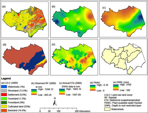
Figure 4. Spatial distribution of the input data for estimating the green and blue water flows of the upper Awash basin for the year 2010.

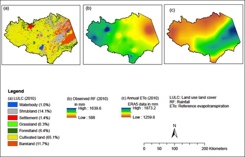
Figure 5. Spatial distribution of the input data for estimating the green and blue water flows of the upper Awash basin for the year 2020.

2.3.5. The seasonal parameter (Z)

The climate seasonality factor reflects the local rainfall patterns and hydrogeologic characteristics ranging from 1 to 30 (Sharp et al. 2014; Yin et al. 2020). Donohue et al. (2012) indicated that Z is positively correlated with the average annual number of rainfall events, and is computed using Equation (2)(2) $$Z=\frac{N}{5}$$(2) (Hamel and Guswa 2015; Yang et al. 2019). (2) $$Z=\frac{N}{5}$$(2) where N is the number of rainfall events (>1 mm) in a given year.

The average number of rainy days in 22 stations of the upper Awash basin was 110, giving a value of 22, which was considered as a Z value.

2.3.6. Green-blue water availability computations

The BWF estimation in InVEST model was conducted using the water balance principle and Budyko curve (Budyko 1974; Gerrits et al. 2009; Haghdadi 2018). It calculates the quantity of water flowing through each pixel as rainfall, subtracting the fraction of water that is subject to evapotranspiration. The annual BWF ($\Upsilon$ (x)) for each pixel on landscape x was computed using Equation (3)(3) $$\Upsilon (x)=\left(1-\frac{\mathit{AET}(x)}{P(x)}\right)\times P(x)$$(3) (Yang et al. 2019). (3) $$\Upsilon (x)=\left(1-\frac{\mathit{AET}(x)}{P(x)}\right)\times P(x)$$(3) where AET(x) is the annual actual evapotranspiration (GWF) for pixel x; and P(x) is the annual rainfall on pixel x.

The InVEST model associates AET with potential evapotranspiration (PET), and the pixel-based evapotranspiration fraction of the vegetated LULC was calculated as Equation (4)(4) $$\frac{\mathit{AET}(x)}{P(x)}=1+\frac{\mathit{PET}(x)}{P(x)}-{\left[1+{\left(\frac{\mathit{PET}(x)}{P(x)}\right)}^{\omega }\right]}^{\frac{1}{\omega }}$$(4) (Zhang et al. 2004; Redhead et al. 2016; Haghdadi et al. 2018; Pathak et al. 2019). (4) $$\frac{\mathit{AET}(x)}{P(x)}=1+\frac{\mathit{PET}(x)}{P(x)}-{\left[1+{\left(\frac{\mathit{PET}(x)}{P(x)}\right)}^{\omega }\right]}^{\frac{1}{\omega }}$$(4) where PET (x) is the potential evapotranspiration at pixel x and is given in Equation (5)(5) $$\mathit{PET}(x)=K_c(l_x)\times E{T}_o(x)$$(5) ; and ω(x) is a non-physical parameter characterizing the natural climatic and soil properties. (5) $$\mathit{PET}(x)=K_c(l_x)\times E{T}_o(x)$$(5) where ETo (x) is the reference evapotranspiration from pixel x and K_c(l_x) is the plant evapotranspiration coefficient associated with the LULC on pixel x (Table 2).

Donohue et al. (2012) proposed an equation to compute the non-physical parameter ω(x) as given in Equations (6)(6) $$\omega (x)=Z\left(\frac{\mathit{AWC}(x)}{P(x)}\right)+1.25$$(6) and (7)(7) $$\mathit{AWC}=\min (\max \hspace{0.17em}\mathit{soil}\hspace{0.17em}\mathit{depth},\mathit{root}\hspace{0.17em}\mathit{depth})\times \mathit{PAWC}$$(7) . (6) $$\omega (x)=Z\left(\frac{\mathit{AWC}(x)}{P(x)}\right)+1.25$$(6) (7) $$\mathit{AWC}=\min (\max \hspace{0.17em}\mathit{soil}\hspace{0.17em}\mathit{depth},\mathit{root}\hspace{0.17em}\mathit{depth})\times \mathit{PAWC}$$(7) where AWC (x) is the volumetric (mm) plant-available water content (Kusratmoko and Semedi 2019).

2.3.7. Green water storage (GWS)

The effective rainfall (P_eff), which is usable for vegetation growth, is considered to be soil water (GWS) depending on the root zone depth and soil storage capacity (Hirpa et al. 2022). For this study, the United States Department of Agriculture (USDA)Soil Conservation Services method was used to compute the GWS (Smith 1992; FAO 2009), as given in Equations (8)(8) $$P_{\mathit{eff}}=\frac{(P\times (125-0.2\times 3\times P))}{125},\mathit{for}P\le \frac{250}{3}$$(8) and (9)(9) $$P_{\mathit{eff}}=\left(\frac{125}{3}\right)+0.1\times P,\mathit{for}P>\frac{250}{3}$$(9) . (8) $$P_{\mathit{eff}}=\frac{(P\times (125-0.2\times 3\times P))}{125},\mathit{for}P\le \frac{250}{3}$$(8) (9) $$P_{\mathit{eff}}=\left(\frac{125}{3}\right)+0.1\times P,\mathit{for}P>\frac{250}{3}$$(9) where P_eff = effective dependable rainfall (mm/dekad); and P = dependable rainfall (mm/dekad). Subsequently, these values were converted into monthly and annual basis values.

2.3.8. Model validation

The annual BWF estimate was validated with the observed annual runoff for each watershed between 2000 and 2010 using hydrological model evaluation criteria. The criteria used for this study are coefficient of determination (R²), Nash-Sutcliffe efficiency (NSE), percent bias (PBAIS) and root mean square error (RMSE)-observation standard deviation ratio (RSR) as indicated in Equation (10)–(13) (Nash and Sutcliffe 1970; Moriasi et al. 2007; Thirel et al. 2015; Adane et al. 2021). (10) $$R^2=\left(\frac{\sum _{i=1}^n(BW{F}_{\mathit{obs},i}-\overline{BW{F}_{\mathit{obs}}})(BW{F}_{\mathit{sim},i}-\overline{BW{F}_{\mathit{sim}}})}{\sqrt{\sum _{i=1}^n{(BW{F}_{\mathit{obs},i}-\overline{BW{F}_{\mathit{obs}}})}^2}\sqrt{\sum _{i=1}^n{(BW{F}_{\mathit{sim},i}-\overline{BW{F}_{\mathit{sim}}})}^2}}\right){}^2,$$(10) (11) $$\mathit{NSE}=1-\frac{\sum _{i=1}^n(BW{F}_{\mathit{obs},i}-BW{F}_{\mathit{sim},i}{)}^2}{\sum _{i=1}^n{(BW{F}_{\mathit{obs},i}-\overline{BW{F}_{\mathit{obs}}})}^2},$$(11) (12) $$\mathit{PBIAS}=\left[\frac{\sum _{i=1}^n(BW{F}_{\mathit{obs},i}-BW{F}_{\mathit{sim},i})}{\sum _{i=1}^n(BW{F}_{\mathit{obs},i})}*100\right],$$(12) (13) $$\mathit{RSR}=\frac{\mathit{RMSE}}{\mathit{STDE}{V}_{\mathit{obs}}}=\frac{\left[\sqrt{\sum _{i=1}^n{(BW{F}_{\mathit{obs},i}-BW{F}_{\mathit{sim},i})}^2}\right]}{\left[\sqrt{\sum _{i=1}^n{(BW{F}_{\mathit{obs},i}-\overline{\mathit{BWF}})}^2}\right]}$$(13) where BWF_obs,i is the i^th year observed BWF, BWF_sim,i is the i^th year simulated BWF by the InVEST model, $\overline{BW{F}_{\mathit{obs}}}$ is the mean observed BWF, and n is the total number of observations in years, $\mathit{STDE}{V}_{\mathit{obs}}$ is the observed standard deviation. The performance rating for the model evaluation criteria is indicated in Table 3.

Table 3. Model validation criteria (Moriasi et al. 2007).

Rating	NSE	PBIAS (%)	RSR
Very good	0.75 ≤ NSE ≤ 1.00	PBIAS < ±10	0.00 ≤ RSR ≤ 0.50
Good	0.65 < NSE ≤ 0.75	±10 ≤ PBIAS < ±15	0.50 < RSR ≤ 0.60
Satisfactory	0.50 < NSE ≤ 0.65	±15 ≤ PBIAS < ±25	0.60 < RSR ≤ 0.70
Unsatisfactory	NSE ≤ 0.50	PBIAS ≥ ±25	RSR > 0.70

2.3.9. Agricultural water scarcity

In this study, the Water Scarcity Index (WSI) has been assessed using the water footprint approach, as a ratio of the total water footprints to water availability in a specific catchment (Hoekstra et al. 2011, 2012; Zeng et al. 2013; Xie et al. 2020; Shu et al. 2021). The green and blue WFs of various irrigated and rainfed crops in the basin and LULC data were used for the analysis (Hirpa et al. 2022). In addition, the 11-year average of BWF from the cultivated land was extracted using GIS and considered as WR_blue in the specific study sites (Debreziet, Wonji, Melkassa and Metehara). Similarly, the average GWS, which was computed using the USDA effective rainfall method, is considered as the green water resource availability (WR_green) and extracted and quantified for cultivated land. These water scarcity indices (WSI_green and WSI_blue) were determined for the dominant rainfed crops (Teff and Maize in Deberezeit, Maize in Wonji, Sorghum and Maize in Melkassa) and irrigated sugarcane in Wonji (SC-1 and SC-2, with 24-months and 14-months length of growing periods (LGPs), respectively), and in Metehara (SC-3 and SC-4, with 20-months and 14-months LGPs, respectively).

The WSI for the cultivated land is computed using Equations (14)(14) $$\mathit{WSI}=\frac{WF}{\mathit{TWR}}$$(14) and (15)(15) $$\mathit{TWR}=\mathrm{}W{R}_{\mathit{blue}}+W{R}_{\mathit{green}}$$(15) (Hoekstra et al. 2011, 2012; Zeng et al. 2013; Xie et al. 2020; Shu et al. 2021): (14) $$\mathit{WSI}=\frac{WF}{\mathit{TWR}}$$(14) (15) $$\mathit{TWR}=\mathrm{}W{R}_{\mathit{blue}}+W{R}_{\mathit{green}}$$(15) where WF is the water footprint of the irrigated or rainfed crops in m³; TWR is the total water resource availability from cultivated land in m³; WR_blue and WR_green are the blue and green water resources for agricultural production in m³.

The green and blue water scarcity for rainfed and irrigated areas are quantified using Equations (16)(16) $$WS{I}_{\mathit{green}}=\mathrm{}\mathrm{}\frac{W{F}_{\mathit{green}}}{W{R}_{\mathit{green}}}$$(16) and (17)(17) $$WS{I}_{\mathit{blue}}=\mathrm{}\mathrm{}\frac{W{F}_{\mathit{blue}}}{W{R}_{\mathit{blue}}}$$(17) : (16) $$WS{I}_{\mathit{green}}=\mathrm{}\mathrm{}\frac{W{F}_{\mathit{green}}}{W{R}_{\mathit{green}}}$$(16) (17) $$WS{I}_{\mathit{blue}}=\mathrm{}\mathrm{}\frac{W{F}_{\mathit{blue}}}{W{R}_{\mathit{blue}}}$$(17) where WSI_green is the green water scarcity index (a dimension less unit) and indicates the ability of crops to consume green water exclusively from rainfall resources. WF_green is the green water footprint (in m³) for the rainfed crops (Teff, maize and sorghum) at Debrezeit, Wonji and Melkassa (Hirpa et al. 2022). WF_blue is the blue water footprint (in m³) used to irrigate sugarcane in Wonji and Metehara. WSI_blue is the blue water scarcity index defined as the ratio of WF_blue to the available blue water resources (WR_blue) for agricultural production.

It should be noted that the environmental flow in the cultivated land is ignored with the assumption that a quantified regulated amount of blue water (irrigation water) is supplied to the farmlands in Wonji and Metehara sugar plantation schemes. Finally, the WSI_blue and WSI_green are characterized for cultivated land based on water scarcity severity indices ranked as per the classification of Hoekstra et al. (2012) and Xie et al. (2020) (Table 4).

Table 4. Water scarcity index ranges (Hoekstra et al. 2012; Xie et al. 2020).

Range	WSIblue type	Range	WSIgreen type
WSIblue < 1	Low water stress	WSIgreen < 0.5	Low water stress
1 ≤ WSIblue < 1.5	Moderate water stress	0.5 ≤ WSIgreen < 1	Moderate water stress
1.5 ≤ WSIblue ≤2	Significant water stress	1 ≤ WSIgreen ≤ 1.5	Significant water stress
WSIblue > 2	Severe water stress	WSIgreen > 1.5	Severe water stress

3. Results

3.1. Model accuracy

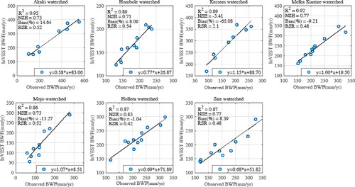
The coefficient of determination (R²) of the BWF of the observed and simulated values in all watersheds shows a lower error variance with a value above 0.85. However, this line of fit is not a guarantee of how well the InVEST model predicts in a watershed. For example, in Kessem, a semi-arid and bareland dominated watershed, the BWF is overestimated, with a negative NSE value (i.e. the means of the observed data predicts better than the model), a high bias, and high RSR values (Figure 6). Thus, unlike the other watersheds, the evaluation of model performance in the Kessem watershed is unsatisfactory. However, the performance rating of the BWF estimates displays ‘good and/or very good’ in all the criteria for the other watersheds (Figure 6).

Figure 6. Validation of the blue water flow at different watersheds in the upper Awash basin.

3.2. Spatio-temporal distribution of the physical and climatic parameters

3.2.1. LULC change during 2000–2020

The percentage of LULC changes (% initial changes) in the past two decades (2000–2020) indicates a staggering expansion in settlement (432% increment with an average annual rate of 17%), cultivated land (42% increment with an average annual rate of 3.5%), and waterbodies (2.4% expansion) (Hirpa et al. 2023). Meanwhile, shrubland, grassland, bare land, and forestland showed a reduction of 44%, 65%, 65%, and 66%, respectively. Therefore, these land-use dynamics and climatic variations in different years are determining factors for the available green-blue water resource variation in the basin. The decadal LULC areal coverages and percent share between 2000 and 2020 are shown in Table 5 and Figures 3–5.

Table 5. Land use land cover areal coverage and percent share in the upper Awash basin (Hirpa et al. 2023).

LULC classes	Land use area (ha)			Land use share (%)
	2000	2010	2020	2000	2010	2020
WB	22,662	23,943	23200	1.0	1.0	1.0
SL	321,549	335,275	180,799	13.5	14.1	7.6
ST	13,782	33,348	73,271	0.6	1.4	3.1
GL	35,763	6,029	12,551	1.5	0.3	0.5
FL	214,682	152,068	72,919	9.0	6.4	3.1
BL	460,151	277,490	159,266	19.4	11.7	6.7
CL	1,307,523	1,547,958	1,854,106	55.0	65.1	78.0

WB: Water body; SL: Shrubland; ST: Settlement; GL: Grassland; FL Forest land; BL: Bareland; CL: Cultivated land.

3.2.2. Climatic and soil parameters

The spatial annual rainfall of the basin ranged from 493–1244 mm, 588–1639 mm, and 545–1527 mm in 2000, 2010, and 2020, respectively. The annual reference evapotranspiration of the basin is higher in the rift watersheds and relatively lower in the highland watersheds. The soil depth of the basin ranged between 100 mm and 3100 mm, with the fraction of PAWC values ranging between 0 and 0.18 (Figures 3–5).

The average gridded pixel rainfall condition in the upper Awash basin showed an increment from 886 mm in 2000 to ∼1050 mm in 2020 (Table 6). This may be due to the influence of ITCZ on the MER and/or on some parts of the central highlands which experiences more wet periods during the small rainy seasons in March-April-May (Adane et al. 2020a). This basin is dominated by highlands to the west, which receive more rainfall and consequently produce more BWF (Adane et al. 2021). In contrast, below-average rainfall during the main rainy season (June-July-August-September) in the basin can be attributed to the alteration in the El Nino phenomenon (Alemu et al. 2017). This condition agree with the findings of Ahmadalipour et al. (2019) and Ayugi et al. (2022) on the future projection in eastern Africa, which generally shows a ‘dry get drier and wet gets wetter’ condition.

Table 6. Decadal hydro-climatic conditions and green and blue water flow in upper Awash basin.

Basin	Year	Area (km^2)	MAR in mm/yr	PET in mm/yr	GWF in mm/yr	BWF in mm/yr	BWF (x10^6) (m^3/yr)
Upper Awash Basin	2000	23761	885.98	1076.74	676.68	208.42	4950.34
	2010		1035.51	1161.73	757.14	277.42	6589.10
	2020		1048.38	1438.50	820.86	226.14	5371.13

MAR: Mean annual rainfall; PET: Potential Evapotranspiration; GWF: Green Water Flow; BWF: Blue Water Flow.

Among the nine watersheds, the highest average rainfall for the observed period was observed in Holleta and Melka Kuntire, and the lowest was recorded in Metehara. The annual PET, which considers a non-physical parameter record of more than ∼1116 mm in 2010 (Akaki watershed) and a maximum of 1422 mm in 2009 (Hombole watershed), was detected considering the seven watersheds excluding Metehara (∼737 mm/yr) and Kessem (∼868 mm/yr), where bareland and sparse shrublands were dominant (Figure 7a and b). The expansion of large-scale sugarcane plantations (in Wonji, Kessem, and Metehara sugar estate farms) and small-scale irrigation farms in the central rift watersheds may have contributed to the increase in PET in 2010 and 2020 in the Koka, Sire, Kessem, and Metehara watersheds (Table S1). Furthermore, the interannual coefficient of variability (CV) of the rainfall among the nine watersheds ranged between ∼12% in Sire and ∼19% in the Holleta watersheds. Meanwhile, the lowest CV of PET was recorded in Akaki (2.43%) and the highest in Kessem (∼10%) (Table 7).

Figure 7. Box plot showing the median, quantile, and range of (a) annual rainfall; (b) annual potential evapotranspiration (PET); (c) annual green water flow (GWF); and (d) blue water flow (BWF) distributions of the upper Awash basin. Aka: Akaki; Hom: Hombole; Kes: Kessem; Kok: Koka; met: Metehara; Moj: Mojo; NHo: Holleta; Sir: Sire.

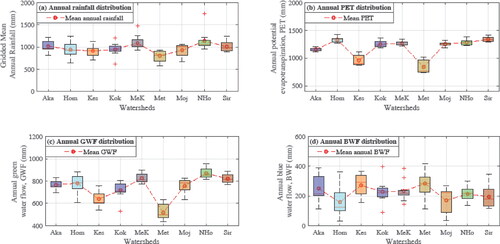
Table 7. Interannual variability of hydroclimatic variables in the upper Awash basin between 2000 and 2010.

Hydro-climatic Components	Coefficient of variation in watersheds (%)
	Aka	Hom	Kes	Kok	MeK	Met	Moj	Hol	Sir
Rainfall	12.36	17.53	13.91	15.18	14.80	15.92	15.46	19.22	11.84
PET	2.43	3.82	9.77	4.92	3.12	14.02	3.13	3.96	3.11

Aka: Akaki; Hom: Hombole; Kes: Kessem; Kok: Koka; Met: Metehara; Moj: Mojo; Hol: Holleta; Sir: Sire.

GWF in all watersheds increased from 2000 to 2020 (Table S2). The annual GWF considering these decadal records depicts a lower value in the Metehara (434 mm in 2002) and a maximum in the Holleta (955 mm in 2006) watersheds (Figure 7c). The lowest average annual BWF was in Hombole (158 mm/yr) and the highest in Metehara (283 mm/yr) (Figure 7d).

3.3. Spatio-temporal green-blue water availability

The highland watersheds experienced a higher GWF than the eastern part of the basin (Figure 8). In addition, the GWF increased with the expansion of the cultivated land in the central rift watersheds, and it was 677 mm/yr in 2000, 757 mm/yr in 2010, and 821 mm/yr in 2020 (Table 6). However, a lower GWF was observed in urban areas where settlements are dominant (Figure 8a, c, and e). The average BWF increased from 2000 (∼208 mm/yr) to 2010 (∼277 mm/yr) and showed a modest decline in 2020 (∼226 mm/yr) over the entire basin (Table 6 and Figure S1). The decline in BWF may be due to the increasing consumption of water for urban supply and the expansion of the cultivated land in the central and eastern parts of the basin.

Figure 8. Spatial and temporal variation of available water resources in the upper Awash basin: (a to f) the decadal green and blue water flow; (g-i) 12–years average blue and green water flows and green water storage across the basin, respectively.

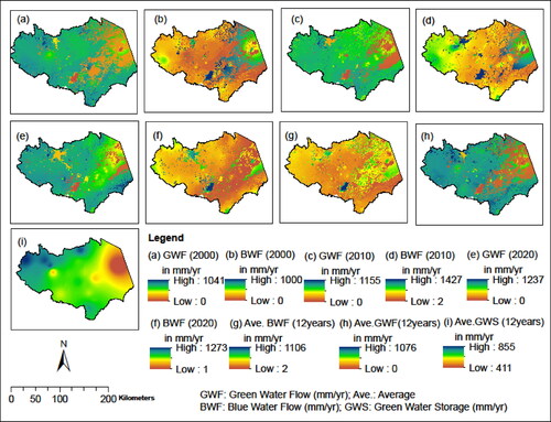
The interannual variability of GWF in the highlands (Akaki, Melka Kuntire, Holleta and Sire) shows less variability (<5%), whereas the remaining watersheds (Mojo, Hombole, Kessem, Koka and Metehara) have shown ∼9–14% of CV (Table 8). The BWF experienced higher interannual variability, with a CV ranging between ∼23% in Holleta and ∼50% in Hombole watersheds (Table 8). The highest average BWF with 1106 mm/yr was exhibited near the water body of the Koka watershed and a relatively high GWF was observed in the western part of the basin where more vegetation cover is dominant (Figure 8). This finding agrees with the spatial map developed for blue and green water resources in Africa by Schuol et al. (2008). Their results based on the developed spatial CV ranges of the average BWF at 95% prediction uncertainty using SWAT model were between 21–50% in the upper, 51–100% in the middle, and 101–200% in the lower Awash basins. Similarly, the CV of the average GWF for the entire Awash basin was within the range of 1–20% (Schuol et al. 2008).

Table 8. Interannual variability of blue and green water flow in the upper Awash basin between 2000 and 2010.

Freshwater Components	Coefficient of variation in watersheds (%)
	Aka	Hom	Kes	Kok	MeK	Met	Moj	Hol	Sir
GWF	4.76	10.02	10.77	10.37	4.81	13.88	8.98	4.92	4.93
BWF	36.13	50.47	27.90	32.60	29.35	31.81	46.63	22.75	38.66

Aka: Akaki; Hom: Hombole; Kes: Kessem; Kok: Koka; Met: Metehara; Moj: Mojo; Hol: Holleta; Sir: Sire.

3.3.1. Green water flow and green water storage in different land uses and watersheds

Among the nine watersheds, the highest average GWF is observed in the highland and central rift watersheds such as Holleta (905 mm/yr), Sire (869 mm/yr), Melka Kuntire (866 mm/yr), Hombole (849 mm/yr), Mojo (801 mm/yr), and Akaki (777 mm/yr). However, a relatively lower GWF was observed in the central and eastern parts of the Awash basin (757 mm/yr in Koka, 704 mm/yr in Kessem, and 598 mm/yr in Metehara) (Figure 9a).

Figure 9. The decadal green water flow (GWF) and green water storage (GWS) in different watersheds (a and b) and in different LULC (c and d) of the upper Awash basin. Ho: Holleta watershed; Sir: Sire watershed; MeK: Melka-Kuntire watershed; Hom: Hombole watershed; Moj: Mojo watershed; Aka: Akaki watershed; Kok: Koka watershed; Kes: Kessem watershed; Met: Metehara watershed. FL: Forestland; CL: Cultivated land; GL: Grassland; SL: Shrubland; Set: Settlement; BL: Bare land; WB: Waterbody.

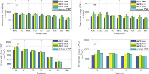
Based on the LULC conditions of the basin, the highest GWF is experienced in forestland (8,438.4 m³/ha in 2000, 9,638.5 m³/ha in 2010, and 10,139 m³/ha in 2020) across all decades. The GWF then declined in the following order: cultivated land, grassland, shrubland, settlement, bareland, and waterbody (Figure 9c and Table 9). Notably, cultivated land in the basin expanded significantly during 2000–2020, at the expense of shrubland, forestland, and bareland. As a result, the GWF in cultivated land increased from ∼8000 m³/ha/yr to 8827 m³/ha/yr and later showed a moderate decline in water availability in 2020 (8815 m³/ha/yr). The lowest GWF observed in the waterbody ranged from 21.9 m³/ha/yr in 2010 to 34.1 m³/ha/yr, indicating a relatively increasing trend compared to the GWF observed in 2000 and 2010 (see Figure 9c and Table 9).

Table 9. Green water flow for different land uses in the upper Awash basin.

Land use class	2000	2010	2020
	GWF (m^3/ha/yr)	GWF (m^3/ha/yr)	GWF (m^3/ha/yr)
WB	24.2	21.9	34.1
SL	7213.4	7585.1	7174.0
ST	4969.0	4681.6	4956.7
GL	7516.5	8196.9	8123.8
FL	8438.4	9638.5	10139.0
BL	3013.1	2947.0	3076.0
CL	7996.0	8826.9	8815.0

WB: Water body; SL: Shrubland; ST: Settlement; GL: Grassland; FL Forest land; BL: Bareland; CL: Cultivated land.

The highest average GWS was experienced in the western and central parts of the basin, i.e. the Holleta (872 mm/yr), Melka Kuntire (855 mm/yr), and Akaki (809 mm/yr) watersheds. In contrast, the lowest values were noted in the semi-arid areas of the Kessem (687 mm/yr) and Metehara (630 mm/yr) watersheds (Figure 9b). The average GWF depths in the decadal periods exhibited a decline in forestland, cultivated land, grassland, shrubland, settlement, and bareland. Conversely, the average GWS in volume per unit hectare of land per year was higher in grassland, and declined in cultivated land, forestland, and shrubland in descending order (Figure 9c and d).

The 12 years-time-series of GWS in the basin showed that the three lowest values were recorded in 2001 (271 mm), 2002 (238 mm), and 2009 (116 mm) in the eastern part of the basin (Figure S2). During this period, continuous dry spells and severe droughts were recorded in these years (Adane et al. 2020a). Additionally, the 12-year average GWS showed a maximum of 855 mm in the western parts of the basin and a minimum of 411 mm in the eastern part (Figure 8i).

3.3.2. Blue water flow in different land uses and watersheds

The highland watersheds of Melka Kuntire, Akaki, and Holleta showed the three highest annual average BWF of 304, 298, and 277 mm/yr, respectively. Intermediate values of annual average BWF were recorded in Koka (246 mm/yr), Sire (234 mm/yr), and Metehara (228 mm/yr) watersheds. In contrast, the three lowest BWF values are from the Kessem (208.2 mm/yr), Hombole (∼198 mm/yr), and Mojo (∼187 mm/yr) watersheds (Figure 10a). The lowest annual BWF was recorded in the area where vegetation covers dominated land uses such as forestland (91 mm/yr), shrubland (161 mm/yr), and cultivated land (180 mm/yr). In contrast, the highest annual BW in depth was recorded in waterbody, settlement, bareland, and grassland at 897, 639, 556, and 369 mm/yr, respectively (Figure 10b). Likewise, the average volume of BWF per hectare of land showed a similar pattern to that of the BWF depth per annum (Figure 10c and Table 10). Cultivated land has the largest share among the seven land use types, with 55% in 2000, ∼65% in 2010, and ∼78% in 2020 (Table 5). As a result, the highest average annual volume of BWF was recorded in the land uses that are having largest share such as cultivated land (∼2.9 billion m³/yr) and bareland (1.64 billion m³/yr), and the remaining land use covers produce an annual average flow of ∼1.1 billion m³/yr (Figure 10d and Table 10). The decadal BWF in the basin was 4.95 billion m³ in 2000, 6.59 billion m³ in 2010, and 5.37 billion m³ in 2020 with an annual average BWF of 5.64 billion m³ (Table 10).

Figure 10. The decadal blue water flows (BWF) in (a) different watersheds of the upper Awash basin; and (b to d) LULC. MeK: Melka Kuntire sub-basin, Aka: Akaki watershed; Ho: Holleta watershed; Kok: Koka watershed; Sir: Sire watershed; Met: Metehara watershed; Kes: Kessem watershed; Hom: Hombole watershed; Moj: Mojo watershed. FL: Forestland; CL: Cultivated land; GL: Grassland; SL: Shrubland; Set: Settlement; BL: Bare land; WB: Waterbody.

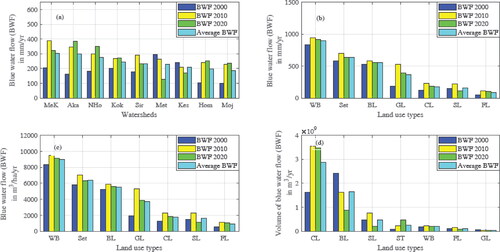
Table 10. BWF Proportions in different land uses and years in the upper Awash basin.

Land classes	BWF2000 (m^3/ha)	BWF2000 in m^3 (x10^9)	BWF2010 in (m^3/ha)	BWF2010 in m^3 (x10^9)	BWF2020 in (m3/ha)	BWF2020 in m^3 (x10^9)	Average BWF in m^3 (x10^9)
WB	8302.1	0.19	9463.4	0.23	9158.5	0.21	0.21
SL	1457.6	0.47	2262.7	0.76	1106.5	0.20	0.48
ST	5836.7	0.08	7016.1	0.23	6317.9	0.46	0.26
GL	1897.3	0.07	5286.2	0.03	3885.8	0.05	0.05
FL	535.1	0.11	1109.8	0.17	1083.6	0.08	0.12
BL	5241.3	2.41	5857.7	1.63	5569.2	0.89	1.64
CL	1237.9	1.62	2289.3	3.54	1877.4	3.48	2.88
Total	24507.9	4.95	33285.4	6.59	28998.9	5.37	5.64

BWF: Blue water flow; WB: Waterbody; SL: Shrub land; ST: Settlement; GL: Grassland; FL: Forest land; BL: Bare land; CL: Cultivated land.

3.4. Agricultural water scarcity

3.4.1. Green water scarcity index for rainfed crops

The green water resources exclusively from GWS (effective rainfall) are mainly consumed by the dominant rainfed crops in the basin. The WSI_green for maize ranges between low water stress (∼0.4 in Wonji and Melkassa) to moderate water stress in Debrezeit (0.50) (Table 11). Teff in Debrezeit and sorghum in Melkassa region show moderate and low water scarcity with WSI_green of 0.51 and 0.4, respectively (Table 11). In general, the rainfed crops experienced moderate green water stress in Debrezeit due to large areas of cultivated land covered by high water footprint crops likes teff, compared to Wonji and Melkassa, which experienced a low green water scarcity. Thus, the WSI_green values indicate that there is a need for enhancing crop management practices, and development of green infrastructure such as detention ponds, percolation pits etc., in order to use the moisture for the dry seasons and increase the yield by reducing the WFs (Hirpa et al. 2023).

Table 11. Green water scarcity index of the rainfed crops in upper Awash basin.

Areas	Rainfed crops	Area (ha)	Av. WFgreen^a x 10^8 (m^3)	WRgreen^b x10^8 (m^3)	WSIgreen^c	WSI level
Debrezeit	Teff	190,818	8.05	15.9	0.51	Moderate
	Maize		7.96		0.5	Moderate
Wonji	Maize	58,544	2.16	5.98	0.36	Low
Melkassa	Maize	94,571	3.63	9.05	0.4	Low
	Sorghum		3.63		0.4	Low

^a AV. WFgreen is the average green water footprint (Hirpa et al. 2022).

^b WR_green is green water resource quantified based on the average green water storage.

^c WSI_green is the green water scarcity index.

3.4.2. Blue water scarcity index for irrigated sugarcane

The WSI_blue for irrigated sugarcane (late maturing crops having a 20 or 24-months LGP) in Wonji and Metehara records above moderate blue water scarcity (Table 12).

Table 12. Blue water scarcity index of the irrigated sugarcane in upper Awash basin.

Areas	Irrigated crops	Area (ha)	Av. WFblue^a x10^8 (m^3)	WRblue^b x 10^8 (m^3)	WSIblue^c	WSI level
Wonji	SC-1^d	12,800	2.34	1.56	1.5	Significant
	SC-2^e		1.36		0.87	Low
Metehara	SC-3^f	10,230	2.15	2.37	1	Moderate
	SC-4^g		1.52		0.64	Low

^aAv. WF_blue is average blue water footprint (Hirpa et al. 2022).

^bWR_blue is the blue water resource from runoff yield.

^cWSI_blue is the blue water scarcity index.

^dSC-1 is sugarcane variety with length of growing periods (LGPs) of 24-month in Wonji.

^eSC-2 is sugarcane variety with LGP of 14-month in Wonji.

^fSC-3 is sugarcane variety with LGPs of 20-month in Metehara; ^gSC-4 is sugarcane variety with LGPs of 14-month in Metehara.

The long LGP sugarcane varieties both in Wonji (SC-1 with WF of 212 m³/ton) and Metehara (SC-3 with WF of 167 m³/ton) experienced WSI_blue of 1.5 and 1.0, which are considered to be significant and moderate blue water scarcity, respectively (Table 12, Hirpa et al. 2022). The water use in m³ per hectare of land for irrigated crops is ∼18,260 m³/ha in SC-1 and ∼21,033 m³/ha in SC-3 and the vast areal coverage of the sugarcane plantation contributed to water scarcity relative to the available blue water resources potential (Table 7.3). The short LGP sugarcane varieties in Wonji (SC-2 with WF of 125 m³/ton) and Metehara (SC-4 with WF of 117 m³/ton) depicted a low blue water scarcity (Table 12, Hirpa et al. 2022). Similarly, the water use in m³ per hectare of land for irrigated crops is ∼10,596 m³/ha in SC-2 (Wonji) and ∼14,819 m³/ha in SC-4 (Metehara) and has low water scarcity relative to the available blue water resources potentials. Combining the green water resources (the green water storage from rainfall) with blue water could reduce the scarcity index from significant to moderate blue water scarcity (0.51 in SC-1), and from moderate to low blue water scarcity (∼0.3 in SC-3) in the upper Awash basin.

4. Discussion

4.1. Green and blue water resource availability

Global freshwater consumption for various purposes has been increasing and will continue to increase, particularly with the expansion of agriculture which is required to satisfy the ever-increasing food demand of the growing population of the world. This has forced one-third of the global population to live in water-scarce areas (Dessu et al. 2014; Khan et al. 2021). Similarly, the agricultural sector consumes ∼70% of the available freshwater use and will significantly increase by 5600 km³/yr by 2050 (Rockström and Barron 2007; Fader et al. 2011). Schuol et al. (2008) modeled the green and blue water resources of Africa (48 countries) and found high interannual variability BWF in the Sahel, in the Horn of Africa and in southern Africa. Similarly, this continental study recorded the BWF, GWF, and GWS of Ethiopia as ∼87 to 187 mm, ∼555 to 602 mm, and ∼18 to 34 mm, respectively (Schuol et al. 2008). The GWF exceeded more than six times the minimum BWF and more than triple the maximum BWF of Ethiopia (Schuol et al. 2008). Our results at the basin level indicated that the 11-year average annual BWF and GWF ranged from ∼170 to 283 mm and ∼518 to 870 mm, respectively. These variations between our results and those of Schuol et al. (2008) could be attributed to the fact that we used local data inputs (observed climatic data, LULC input with 30 m resolution, soil depth, available water content, and biophysical information) at the watershed level, while Schuol et al. (2008) used average continental/regional data inputs. The difference in the type of hydrological models also contributes to the variations in results. Thus, the results of these two hydrological models particularly in terms of the BWF estimates show discrepancies, where the continental studies underestimated the BWF.

Mekonnen and Hoekstra (2016) stated that two-thirds of the world’s population lives under severe water scarcity conditions for at least one month each year and nearly half a billion people all year round. Rockström et al. (2009) also projected 36% of the global population will face both green and blue water shortages by 2050. Similarly, 59% will face blue water scarcity. In the Awash basin, the blue water demand exceeds the blue water availability and various competing water users (such as for agricultural production, domestic uses, industrial sectors, and environmental flows to sustain the ecology) are encountering water scarcity earlier than anticipated (in 2025) (Barker et al. 1999; Adeba et al. 2015). The available green water resources in the basin could significantly contribute to reducing the risk of consecutive dry spells and drought (Adane et al. 2020a). Similarly, quantification of water use by agriculture, industries and the domestic sector and their contribution to blue water scarcity should be given due attention. Furthermore, integrating green and blue water management assists in sustaining the ecosystem (biodiversity conservation) via maintaining the environmental flows. It will also contribute in addressing food security for the growing population in the basin in alignment with many UN SDGs (SDG 2: ‘Zero Hunger’, SDG 6.6.1: ‘Water for Ecosystem’ and SDG 15: ‘Life on Land’) (Lartey 2015; UNGA 2015; Libala et al. 2022).

4.2. Implications of this study

Large part of the upper Awash basin is cultivated land which shows an increase in total coverage from 2000 (55%) to 2020 (78%) (Hirpa et al. 2023). Adeba et al. (2015) indicated the prevalence of water scarcity in the basin, which resulted from inefficient management, utilization of water resources (blue and green water) for intensive subsistence farming practices on the highlands. On the other hand, the central rift is dominated by both large-and small-scale irrigation schemes, which largely contributed to blue water scarcity in the basin (Hirpa et al. 2022). This study also shows that blue water scarcity for large scale (>22000 ha) irrigated sugarcane in Wonji and Metehara ranges between low to significant water scarcity depending on the sugarcane varieties (14-, 20- and 24-months LGPs). Similarly, the green water scarcity ranges between low to moderate and forces farmers to look for supplementary water by withdrawing groundwater or diverting river water, which could aggregately influence the blue water resources. Agricultural water management practices in the basin usually focus on blue water (irrigation water) management, sidelining the potential of green water availability mainly as a soil moisture reserve that extends the growing periods of the cultivated land and prevents consecutive dry spell influences in the basin. In addition, cultivation of less water consuming varieties (e.g. in SC-2 and SC-4 of 14-months sugarcane), particularly in large scale irrigation schemes, may contribute to minimizing the blue water scarcity. Thus, improving soil water through effective management practices could enhance the green water storage and a careful selection of crop varieties can reduce the stress on the existing blue water resources in the basin. Therefore, as a policy direction for water managers, ecohydrologists, and water users, integrating green and blue water resources is vital for promoting the protection, restoration, and sustainable utilization of water resources in the Awash basin.

4.3. Model and research limitations

In the semi-arid parts of the Awash basin, particularly the Metehara and Kessem watersheds, the BWF should be carefully compared with the outputs of other models, as the InVEST model overestimates the BWF particularly in Kessem watershed. Overestimation of the BWF could be possible in these two semi-arid watersheds (Kessem and Metehara) because of the presence of less vegetation cover and more bareland and the model assigned zero values to the bareland but actually in the ground some rudimentary vegetation cover could be present. Furthermore, the does not differentiate between surface runoff, soil middle flow, and sub-surface flow (Yang et al. 2019). This also could result in overestimation of the BWF. However, the model is under progress with version updates to reduce such uncertainties and overestimation. It is thus necessary to test and compare the green-blue water resources of basins using other distributed or semi-distributed hydrological models.

This study has given more emphasis on quantifying the green-blue water resources and integrating them with agricultural water scarcity but did not address the domestic and industrial water uses and their contribution to water scarcity. Thus far, studies on partitioning of water resource availability and on characterizing agricultural water scarcity from the water footprint perspectives have never been conducted in the basin. It is therefore impossible to compare our model outputs and the resulting agricultural water scarcity estimates. However, we attempted to compare the observed BWF (measured) with the InVEST model output (see Figure 6). Future research should focus on modeling and quantifying the extent of water use by industrial and domestic sectors and their influence on blue water scarcity from a water footprint perspective, which will help to reduce the pressure on blue water resources of the highly industrialized and densely populated basin.

5. Conclusions

The major findings of this study on the spatio-temporal dynamics of green-blue water resource availability in the upper Awash basin using the InVEST model are as follows:

• The highlands and central rift watersheds experienced higher GWF and interannual variability than the eastern rift watersheds during the modeled period.

• Based on vegetation cover, the highest GWF and GWS were experienced in forestland, cultivated land, and grassland, and relative increments in annual GWF were observed with the expansion of cultivated land from 2000 to 2020 in the highland and central rift watersheds. In contrast, settlement, bareland, and impervious layers dominated urban catchments exhibited lower GWF and GWS in the basin.

• The highest annual average BWF depth was observed in the Melka Kuntire, Akaki, and Holleta watersheds, with intermediate annual average BWF in the Koka, Sire, and Metehara watersheds and the lowest in the Kessem, Hombole, and Mojo watersheds, in descending order.

• The total BWF at a decadal interval in different LULC conditions showed an increment from 2000 to 2010 but a modest decline in 2020. This is because of the expansion of the cultivated land of small-scale and large-scale irrigation schemes, particularly in the central rift watersheds. This increased the GWS and reduced the BWF in the basin.

• The GW scarcity indices show low to moderate scarcity for rainfed crops, and moderate to significant BW scarcity for irrigated sugarcane.

• The gridded spatial water availability in different watersheds and LULC conditions, along with understanding the green-blue agricultural water scarcity, helps to design different water storage structures, implement effective moisture conservation practices to increase the GWS in a water-scarce basin, and design sustainable water management strategies to ensure the sustainability of the ecosystem and natural resources of the upper Awash basin. Furthermore, quantifying GWF and GWS helps understand the green water potential in the basin to sustain the food security of small-scale farmers and reduce the impact of BW scarcity in the basin.

• Future research on the influences of industrial and domestic sectors to blue water scarcity from a water footprint perspective is equally important to reduce the pressure on blue water resources of the basin.

Authors contribution

Conceptualization, methodology, data curation and formal analysis: BAH, DN and AA; software: BAH and GBA; Validation: BAH, GBA, MR, CS, DN, AA and W-KL; Resources: BAH, GBA and W-KL; Writing: original draft preparation, BAH and AA; Writing: review and editing, BAH, GBA, MR, CS, DN, AA and W-KL; Supervision: DN and AA; funding acquisition: BAH and W-KL. All authors read and approved the final manuscript.

Acknowledgments

This work is part of the Ph.D. dissertation of the first author (BAH) at the Africa Center of Excellence for Water Management, Addis Ababa University, under the supervision of AA and DN. The authors acknowledge the National Meteorological Services Agency (NMSA), the Ethiopian Ministry of Water and Energy, FAO (for FAO-WaPOR database), and ECMWF's Copernicus Climate Change Service product databases for providing us data free of charge. In addition, we acknowledge Dr. Alemseged Tamiru, Dr. Fasikaw Atanaw and Professor Tenalem Ayenew for their constructive feedback on earlier versions of the manuscript.

Disclosure statement

No potential conflict of interest was reported by the authors.

Additional information

Funding

This study was supported by OJEong Resilience Institute (OJERI) at Korea University under the Basic Science Research Program through the National Research Foundation of Korea (NRF) (NRF-2021R1A6A1A10045235) and the Korea Agency for Infrastructure Technology Advancement (KAIA) grant funded by the Ministry of Land, Infrastructure and Transport (Grant 23UMRG-B158194-04).

References

- Adane GB, Hirpa BA, Gebru BM, Song C, Lee WK. 2021. Integrating satellite rainfall estimates with hydrologicalwater balance model: rainfall-runoff modeling in Awash River Basin, Ethiopia. Water (Switzerland). 13(6):800.
- Adane GB, Hirpa BA, Lim CH, Lee WK. 2020a. Spatial and temporal analysis of dry and wet spells in upper Awash River Basin, Ethiopia. Water (Switzerland). 12(11):3051.
- Adane GB, Hirpa BA, Song C, Lee WK. 2020b. Rainfall characterization and trend analysis of wet spell length across varied landscapes of the upper Awash River Basin, Ethiopia. Sustainability. 12(21):9221. doi: 10.3390/su12219221.
- Adeba D, Kansal ML, Sen S. 2015. Assessment of water scarcity and its impacts on sustainable development in Awash Basin, Ethiopia. Sustain Water Resour Manage. 1(1):71–87.
- Ahmadalipour A, Moradkhani H, Castelletti A, Magliocca N. 2019. Future drought risk in Africa: integrating vulnerability, climate change, and population growth. Sci Total Environ. 662:672–686.
- Allen RG, Pereira LS, Raes D, Smith M. 1998. Crop Evapotranspiration-guidelines for computing crop water requirements-FAO Irrigation and Drainage Paper 56. Vol. 300, Rome, Italy: FAO, p. 6541.
- Alemu A, Korecha D, Mohamod M. 2017. Impacts of various ENSO phases on cereal crop productivity in the upper Awash Basin, Central High Land of Ethiopia. In: Proceedings of the International Conference on Impact of El Nino on Biodiversity, Agriculture and Food Security; p. 23–24.
- Aneseyee AB, Soromessa T, Elias E, Noszczyk T, Feyisa GL. 2022. Evaluation of water provision ecosystem services associated with land use/cover and climate variability in the Winike Watershed, Omo Gibe Basin of Ethiopia. Environ Manage. 69(2):367–383.
- Asad SQ, Tesfaye E, Melese M. 2018. Prospects of alternative copping systems for salt-affected soils in Ethiopia. J Soil Sci Environ Manage. 9(7):98–107.
- Ayugi B, Eresanya EO, Onyango AO, Ogou FK, Okoro EC, Okoye CO, Anoruo CM, Dike VN, Ashiru OR, Daramola MT, et al. 2022. Review of meteorological drought in Africa: historical trends, impacts, mitigation measures, and prospects. Pure Appl Geophys. 179(4):1365–1386. doi: 10.1007/s00024-022-02988-z.
- Báldi A, Vári Á. 2020. Freshwater ecosystems: research, policy and applications. Biol Futura. 71(4):333–336. doi: 10.1007/s42977-020-00051-3.
- Barker R, Seckler D, Amarasinghe UA. 1999. The world’s water: emerging issues in an era of growing scarcity. Choices. Fourth Quarter Special Issue, 28–31.
- Bejagam V, Keesara VR, Sridhar V. 2022. Impacts of climate change on water provisional services in Tungabhadra basin using InVEST Model. River Res Appl. 38(1):94–106.
- Belete M, Deng J, Zhou M, Wang K, You S, Hong Y, Weston M. 2018. A new approach to modeling water balance in Nile River Basin, Africa. Sustainability. 10(3):810.
- Benra F, De Frutos A, Gaglio M, Álvarez-Garretón C, Felipe-Lucia M, Bonn A. 2021. Mapping water ecosystem services: evaluating InVEST model predictions in data scarce regions. Environ Model Softw. 138. doi: 10.1016/j.envsoft.2021.104982.
- Budyko MI. 1974. Climate and life. New York, NY: Academic Press.
- Canqiang Z, Wenhua L, Biao Z, Moucheng L. 2012. Water yield of Xitiaoxi river basin based on InVEST modeling. J Resour Ecol. 3(1):50–54.
- Chen H, Shao M, Li Y. 2008. Soil desiccation in the Loess Plateau of China. Geoderma. 143(1–2):91–100. doi: 10.1016/j.geoderma.2007.10.013.
- Daba MH, You S. 2022. Quantitatively assessing the future land-use/land-cover changes and their driving factors in the upper stream of the Awash River based on the CA–Markov model and their implications for water resources management. Sustainability. 14(3):1538.
- Dennedy-Frank PJ, Muenich RL, Chaubey I, Ziv G. 2016. Comparing two tools for ecosystem service assessments regarding water resources decisions. J Environ Manage. 177:331–340.
- Dessu SB, Melesse AM, Bhat MG, McClain ME. 2014. Assessment of water resources availability and demand in the Mara River Basin. Catena. 115:104–114.
- Donohue RJ, Roderick ML, McVicar TR. 2012. Roots, storms and soil pores: incorporating key ecohydrological processes into Budyko’s hydrological model. J Hydrol. 436–437:35–50.
- Du L, Rajib A, Merwade V. 2018. Large scale spatially explicit modeling of blue and green water dynamics in a temperate mid-latitude basin. J Hydrol. 562:84–102.
- Fader M, Gerten D, Thammer M, Heinke J, Lotze-Campen H, Lucht W, Cramer W. 2011. Internal and external green-blue agricultural water footprints of nations, and related water and land savings through trade. Hydrol Earth Syst Sci. 15(5):1641–1660.
- Falkenmark M, Rockström J. 2006. The new blue and green water paradigm: breaking new ground for water resources planning and management. J Water Resour Plann Manage. 132(3):129–132.
- FAO Land and Water Division. 2009. CROPWAT Software. Available online: https://www.fao.org/land-water/databases-and-software/cropwat/en/.
- Gemechu T. 2014. Estimating the impacts of land use and land cover change on runoff and sediment yield using SWAT model: case study of Keleta watershed, Upper Awash Sub … https://nadre.ethernet.edu.et/record/2828/files/Thesis.pdf.
- Gerrits AMJ, Savenije HHG, Veling EJM, Pfister L. 2009. Analytical derivation of the Budyko curve based on rainfall characteristics and a simple evaporation model. Water Resour Res. 45:W04403. doi: 10.1029/2008WR007308.
- Goldman RL, Benitez S, Calvache A, Davidson S, Ennaanay D, McKenzie E, Tallis H. 2010. Linking people and nature through watershed conservation in the East Cauca Valley, Colombia. In: TEEB D2 case study.
- Haghdadi M, Heshmati G, Azimi MS, Siroosi H. 2018. Simulation of water yield in different plant types based on InVEST Model. In: Третьи Виноградовские Чтения Грани Гидрологии. p. 673–679.
- Haghdadi M. 2018. Assessment of water yield service on the basis of InVEST tool (case study: Delichai watershed). J Water Soil Conserv. 25(4):275–290.
- Halder S, Das S, Basu S. 2022. Estimation of seasonal water yield using InVEST model: a case study from West Bengal, India. Arab J Geosci. 15(14):1–18.
- Hamel P, Guswa AJ. 2015. Uncertainty analysis of a spatially explicit annual water-balance model: case study of the Cape Fear basin, North Carolina. Hydrol Earth Syst Sci. 19(2):839–853.
- Hargreaves GH, Allen RG. 2003. History and Evaluation of Hargreaves Evapotranspiration Equation. J Irrig Drain Eng. 129(1):53–63.
- Hargreaves GH, Samani ZA. 1985. Reference crop evapotranspiration from temperature. Appl Eng Agric. 1(2):96–99.
- Hirpa BA, Adane GB, Asrat A, Nedaw D, Song C, Roh M, Lee W-K. 2023. Urban sprawl at the expense of cultivated land: decadal land use and land cover changes and future projections in the upper Awash basin of central Ethiopia. Front Ecol Evol. 11:1–17. doi: 10.3389/fevo.2023.1160987.
- Hirpa BA, Adane GB, Asrat A, Nedaw D. 2022. Spatio-temporal variability and trend of water footprints in the upper Awash basin, central Ethiopia. J Hydrol. 608:127686.
- Hirpa BA, Adane GB, Asrat A, Nedaw D. 2023. Green, blue and economic water productivity: a water footprint perspective from the Upper Awash Basin, Central Ethiopia. J Water Clim Change. 14(2):559–575. doi: 10.2166/wcc.2023.400
- Hoekstra AY, Chapagain AK, Aldaya MM, Mekonnen MM. 2011. The water footprint assessment manual: setting the global standard. London UK, Washington, DC, USA: Earthscan.
- Hoekstra AY, Chapagain AK, Van Oel PR. 2017. Advancing water footprint assessment research: challenges in monitoring progress towards sustainable development goal 6. Water. 9(6):438.
- Hoekstra AY, Mekonnen MM, Chapagain AK, Mathews RE, Richter BD. 2012. Global monthly water scarcity: blue water footprints versus blue water availability. PLoS One. 7(2):e32688.
- Jafarzadeh AA, Mahdavi A, Shamsi SRF, Yousefpour R. 2021. Assessing synergies and trade-offs between ecosystem services in forest landscape management. Land Use Policy. 111:105741.
- Khan T, Nouri H, Booij MJ, Hoekstra AY, Khan H, Ullah I. 2021. Water footprint, blue water scarcity, and economic water productivity of irrigated crops in Peshawar Basin, Pakistan. Water. 13(9):1249.
- Kusratmoko E, Semedi JM. 2019. Water availability in Patuha mountain region using InVEST Model “hydropower water yield”. In: E3S Web of Conferences. Vol. 125. EDP Sciences; p. 1015.
- Lartey A. 2015. End hunger, achieve food security and improved nutrition and promote sustainable agriculture. UN Chron. 51(4):6–8.
- Lee M-H, Bae D-H. 2015. Climate change impact assessment on green and blue water over Asian monsoon region. Water Resour Manage. 29(7):2407–2427.
- Li Y, Cai Y, Wang X, Li C, Liu Q, Sun L, Fu Q. 2022. Classification analysis of blue and green water quantities for a large-scale watershed of southwest China. J Environ Manage. 321:115894.
- Libala N, Griffin N, Nyingwa A, Dini J. 2022. Freshwater ecosystems and interactions with the SDG 2030 Agenda: implications for SDG implementation in South Africa. Afr J Aquat Sci. 47(3):353–368.
- Liu M, Zhang P, Cai Y, Chu J, Li Y, Wang X, Li C, Liu Q. 2023. Spatial-temporal heterogeneity analysis of blue and green water resources for Poyang Lake basin, China. J Hydrol. 617:128983.
- Liu X, Liu W, Tang Q, Liu B, Wada Y, Yang H. 2022. Global agricultural water scarcity assessment incorporating blue and green water availability under future climate change. Earth’s Futur. 10(4):e2021EF002567.
- Lüke A, Hack J. 2018. Comparing the applicability of commonly used hydrological ecosystem services models for integrated decision-support. Sustainability. 10(2):346.
- Mekonnen MM, Hoekstra AY. 2016. Four billion people facing severe water scarcity. Sci Adv. 2(2):e1500323.
- Moriasi DN, Arnold JG, Van Liew MW, Bingner RL, Harmel RD, Veith TL. 2007. Model evaluation guidelines for systematic quantification of accuracy in watershed simulations. Trans ASABE. 50(3):885–900.
- Nash E, Sutcliffe V. 1970. River flow forecasting through conceptual models part I. A discussion of principles. J Hydrol. 10(3):282–290.
- Pathak S, Ojha CSP, Shukla AK, Garg RD. 2019. Assessment of annual water-balance models for diverse Indian watersheds. J Sustainable Water Built Environ. 5(3):04019002.
- Quinteiro P, Rafael S, Villanueva-Rey P, Ridoutt B, Lopes M, Arroja L, Dias AC. 2018. A characterisation model to address the environmental impact of green water flows for water scarcity footprints. Sci Total Environ. 626:1210–1218
- Rab MA, Chandra S, Fisher PD, Robinson NJ, Kitching M, Aumann CD, Imhof M. 2011. Modelling and prediction of soil water contents at field capacity and permanent wilting point of dryland cropping soils. Soil Res. 49(5):389–407.
- Redhead JW, Stratford C, Sharps K, Jones L, Ziv G, Clarke D, Oliver TH, Bullock JM. 2016. Empirical validation of the InVEST water yield ecosystem service model at a national scale. Sci Total Environ. 569–570:1418–1426.
- Rockström J, Barron J. 2007. Water productivity in rainfed systems: overview of challenges and analysis of opportunities in water scarcity prone savannahs. Irrig Sci. 25(3):299–311.
- Rockström J, Falkenmark M, Karlberg L, Hoff H, Rost S, Gerten D. 2009. Future water availability for global food production: the potential of green water for increasing resilience to global change. Water Resour Res. 45(7):1–16.
- Rockström J, Lannerstad M, Falkenmark M. 2007. Assessing the water challenge of a new green revolution in developing countries. Proc Natl Acad Sci U S A. 104(15):6253–6260.
- Sayyad G, Vasel L, Besalatpour AA, Gharabaghi B, Golmohammadi G. 2015. Modeling blue and green water resources availability in an Iranian data scarce watershed using SWAT. J Water Manage Model. C391:1-8. doi: 10.14796/JWMM.C391.
- Schuol J, Abbaspour KC, Yang H, Srinivasan R, Zehnder AJB. 2008. Modeling blue and green water availability in Africa. Water Resour Res. 44(7):W07406. doi: 10.1029/2007WR006609.
- Scordo F, Lavender TM, Seitz C, Perillo VL, Rusak JA, Piccolo MC, Perillo GME. 2018. Modeling Water Yield: assessing the role of site and region-specific attributes in determining model performance of the InVEST Seasonal Water Yield Model. Water (Switzerland). 10(11):1496.
- Serur AB. 2020. Modeling blue and green water resources availability at the basin and sub-basin level under changing climate in the Weyb River basin in Ethiopia. Sci Afr. 7:e00299.
- Sharp R, Tallis HT, Ricketts T, Guerry AD, Wood SA, Chaplin-Kramer R, Nelson E, Ennaanay D, Wolny S, Olwero N. 2014. InVEST user’s guide. Stanford, CA, USA: The Natural Capital Project.
- Shawul A, Chakma S. 2018. The response of peak discharge and sedimentation to the land use/land cover change scenarios in the Upper Awash basin, Ethiopia. https://www.essoar.org/doi/abs/10.1002/essoar.10500582.1.
- Shawul AA, Chakma S, Melesse AM. 2019. The response of water balance components to land cover change based on hydrologic modeling and partial least squares regression (PLSR) analysis in the Upper Awash Basin. J Hydrol Reg Stud. 26:100640.
- Shu R, Cao X, Wu M. 2021. Clarifying regional water scarcity in agriculture based on the theory of blue, green and grey water footprints. Water Resour Manage. 35(3):1101–1118.
- Smith M. 1992. CROPWAT—A computer program for irrigation planning and management. Irrigation and Drainage Paper 46. Rome, Italy.
- Sordo-Ward A, Granados I, Iglesias A, Garrote L. 2019. Blue water in Europe: estimates of current and future availability and analysis of uncertainty. Water. 11(3):420.
- Swain SS, Mishra A, Sahoo B, Chatterjee C. 2020. Water scarcity-risk assessment in data-scarce river basins under decadal climate change using a hydrological modelling approach. J Hydrol. 590:125260.
- Thirel G, Andréassian V, Perrin C, Audouy J-N, Berthet L, Edwards P, Folton N, Furusho C, Kuentz A, Lerat J, et al. 2015. Hydrology under change: an evaluation protocol to investigate how hydrological models deal with changing catchments. Hydrol Sci J. 60(7–8):1184–1199.
- UNGA. 2015. Transforming our world: the 2030 agenda for sustainable development, 21 October 2015. A /RES/70/1. [accessed 2021 Jul 16]. https://www.un.org/en/development/desa/population/migration/generalassembly/docs/globalcompact/A_RES_70_1_E.pdf.
- UN-Water/Africa. 2006. African water development report 2006. Addis Ababa, Ethiopia: Economic Commission for Africa.
- Vigerstol KL, Aukema JE. 2011. A comparison of tools for modeling freshwater ecosystem services. J Environ Manage. 92(10):2403–2409.
- Wang X, Liu G, Lin D, Lin Y, Lu Y, Xiang A, Xiao S. 2022. Water yield service influence by climate and land use change based on InVEST model in the monsoon hilly watershed in South China. Geomatics Nat Hazards Risk. 13(1):2024–2048.
- Wei P, Chen S, Wu M, Deng Y, Xu H, Jia Y, Liu F. 2021. Using the invest model to assess the impacts of climate and land use changes on water yield in the upstream regions of the Shule River Basin. Water (Switzerland). 13(9):1250.
- Xie P, Zhuo L, Yang X, Huang H, Gao X, Wu P. 2020. Spatial-temporal variations in blue and green water resources, water footprints and water scarcities in a large river basin: a case for the Yellow River basin. J Hydrol. 590:125222.
- Xu C, Zhang W, Wang S, Chen H, Azzam A, Zhang B, Xu Y, Nie N. 2023. Spatiotemporal green water dynamics and their responses to variations of climatic and underlying surface factors: a case study in the Sanjiang Plain, China. J Hydrol Reg Stud. 45:101303.
- Yang D, Liu W, Tang L, Chen L, Li X, Xu X. 2019. Estimation of water provision service for monsoon catchments of South China: applicability of the InVEST model. Landsc Urban Plan. 182:133–143.
- Yin G, Wang X, Zhang X, Fu Y, Hao F, Hu Q. 2020. InVEST model-based estimation of water yield in North China and its sensitivities to climate variables. Water (Switzerland). 12(6):1692.
- Zeng Z, Liu J, Savenije HHG. 2013. A simple approach to assess water scarcity integrating water quantity and quality. Ecol Indic. 34:441–449.
- Zhang L, Hickel K, Dawes WR, Chiew FHS, Western AW, Briggs PR. 2004. A rational function approach for estimating mean annual evapotranspiration. Water Resour Res. 40(2):W02502. doi: 10.1029/2003WR002710.
- Zhang X, Xu Y, Hao F, Li C, Wang X. 2019. Hydrological components variability under the impact of climate change in a semi-arid river basin. Water. 11(6):1122.