Dynamic monitoring of surface water areas of nine plateau lakes in Yunnan Province using long time-series Landsat imagery based on the Google Earth Engine platform

Abstract

Lakes are sensitive to both climate change and human activities, especially in the Yungui Plateau zone. As the main supply of water sources, surface water has a significant impact on environment, ecological balance and socioeconomic development. However, it is unclear how the surface water areas (SWAs) of the nine Yunnan Plateau lakes (NYPLs) have changed over previous decades. In this study, the SWAs of the NYPLs were first extracted using the optimal water index (WI) based on Landsat remote sensing images and the Google Earth Engine (GEE). Then, a spatiotemporal variation analysis of the SWAs was carried out for the NYPLs from 1988 to 2021. Finally, the correlations between the SWA changes in each lake, climatic factors and human activities were analysed. We found that the total SWAs of the NYPL have remained stable over the past 30 years, reaching a maximum of 1,012.51 km² in 2000 and a minimum of 972.94 km² in 2015. From 1988 to 2015, the overall SWAs of the NYPLs fluctuated steadily within 1%. However, Lakes Qilu and Yilong shrunk significantly in 2015. Generally, the SWAs of the NYPLs during the rainy season were larger than during the dry season; however, there were some differences between each period. The seasonal change in the SWAs was approximately 10 km² in 1991, 1994, and 2003, but was relatively less in other years. Precipitation was a direct factor, whereas temperature and evaporation were indirect factors influencing the intra- and inter-annual SWAs of the NYPLs. The changes in the SWAs of the NYPLs were consistent with the precipitation trend and were negatively correlated with changes in temperature and evaporation. Evaporation had more of an influence on shallow lakes than on deep-water lakes. Human activities led to significant changes in individual lakes (such as lakes Dianchi, Yilong, and Qilu). The NYPLs had a spatially heterogeneous response to regional climate change caused by both global climate change and human activities. The results of this study can provide a data reference and decision support for the scientific management of the ecological environment of the Yunnan Plateau lakes.

Keywords:

• Nine Plateau Lakes
• surface water areas
• water index
• Otsu algorithm
• Google Earth Engine

1. Introduction

The ‘Nine Yunnan Plateau Lakes’ (NYPLs) are nine lakes with areas larger than 10 km² in Yunnan Province, China (Qian et al. 2018). The NYPLs are a primary water resource for residents, as well as agricultural and industrial production in Yunnan Province; they also play an irreplaceable role in social and economic development and ecosystem services, especially ecotourism (Wu et al. 2016; Zhou et al. 2019). The surface water areas (SWAs) of lakes are important indicators of regional climate change and anthropogenic activities (Pande 2020; Orimoloye et al. 2022). However, with rapid urbanisation in the NYPL basins and the intensification of regional and global climate change, shrinkage of the NYPLs has occurred in the past 30 years, which has directly influenced regional ecosystem, biodiversity, and water resource balance (Harris 1994; Whitmore et al. 1997; Mishra et al. 2021; Pande et al. 2022). Therefore, monitoring SWA changes in the NYPLs for sustainable economic and social development, ecosystem stability, lake utilisation and protection is important.

Compared with traditional methods, remote sensing has unique advantages for dynamically monitoring lakes at the regional or global scale, owing to its low cost and high frequency and repeatable observations (Xia et al. 2019). Over previous decades, optical satellite imagery (e.g. AVHRR, MODIS, SPOT, Senintel-2, Landsat series, and GF series) has been widely applied to extract SWAs. However, owing to its medium spatial resolution (30 m), multispectral bands, free access, and more than 50 years of observations on global scale, Landsat series data are the most widely used satellite imagery (Wu et al. 2016; Xia et al. 2019; Zhou et al. 2019). Recently, several methods have been proposed for extracting SWA data, including the single-band threshold (Work and Gilmer 1976; White 1978), unsupervised and supervised classification (Yang et al. 2015; Mueller et al. 2016; Ruan et al. 2016; Tulbure et al. 2016), spectral water indexes (Ma et al. 2019), and machine learning (Miao et al. 2018; Wang et al. 2020). Owing to their relatively high accuracy, efficiency and low-cost implementation, several water indices (such as NDWI (Mcfeeters 1996), MNDWI)(Xu 2006), AWEI (Feyisa et al. 2014), NWI (Feng 2012), WI₂₀₁₅ (Fisher et al. 2016)) have been successfully used to map the SWAs of lakes at regional or global scale using Landsat images (Arvor et al. 2018; Aires et al. 2020; Pickens et al. 2020; Worden and de Beurs 2020; Hamunyela et al. 2022; Olthof and Rainville 2022). For example, Wu et al. (2016) adopted the MNDWI and object-based image analysis (OBIA) methods to successfully extract the SWAs of the NYPLs using Landsat images. The experimental results showed that the proposed method obtained satisfactory results compared with those of the visual SWA interpretation. Pekel et al. (2016) produced a 30-m Global Surface Water Dataset (GSWD) from 1984 to 2020 using three million Landsat satellite images, which analysed the distribution and changes in global surface water over the past 36 years. Pickens et al. (2020) produced 30-m global inland water dynamics maps from 1999 to 2018 using a full Landsat time-series, which were mapped and sampled to characterise global inland water dynamics. Fisher et al. (2016) analysed the differences among common water indices used to automatically extract surface water. Their results showed that the classification accuracy of each water index (WI) method is highly dependent on the composition of the validation pixels and heterogeneous backgrounds; each WI is only suitable for specific geographic environments. Various WIs were assessed to identify inland water bodies using Landsat OLI imagery. They showed that obtaining the best results using any WI, corresponding to the different types of inland water bodies (such as clear water, turbid water, and muddy water)remains difficult (Xie et al. 2016). In summary, completing high-accuracy surface water mapping at regional or global scale using a single WI remains complex. Therefore, when mapping surface water at large scale based on the WI, the adaptability of WI should first be analysed for different lakes.

The Google Earth Engine (GEE), which is a free cloud computing, stores several decades of historical remote sensing data (such as MODIS, Landsat, Sentinel, and GF-1) and scientific datasets, enabling parallel computing and feasible big data processing in large study area (Liu et al. 2020a). Recently, The GEE has been successfully applied to forest and crop mapping (Chen et al. 2017; Duan et al. 2019; Oliphant et al. 2019; Phalke et al. 2020; Pan et al. 2021; Guo et al. 2022), land use/cover dynamics (Zurqani et al. 2018; Hao et al. 2019; Pande 2022; Li et al. 2023; Xia et al. 2023), disaster monitoring and assessment (Shinde et al. 2023), and open surface water mapping (Wang et al. 2019; Zhou et al. 2019; Kandekar et al. 2021). Therefore, the GEE can also monitor the long-term dynamics of SWAs on a large scale. For example, a method for surface water extraction based on the GEE was proposed for the long-term surface monitoring of surface water dynamics w in the Middle Yangtze River Basin (Wang et al. 2018). Xia et al. (2019) successfully monitored changes in SWAs from 1989 to 2017 in the Huai River Basin using Landsat data and the GEE. Zhou et al. (2019) used Landsat imagery and the GEE to continuously monitor lake dynamics on the Mongolian Plateau. Wang et al. (2019) proposed an index-and pixel-based water detection method based on the GEE to calculate the inundation frequency of Poyang Lake from 1988 to 2016, comparing the differences in Poyang Lake’s water body between the pre- and post-TGD (Three Gorges Dam) periods.

These studies show that surface water extraction methods based on the GEE have been widely used for the dynamics monitoring of lakes on a large scale. However, the diversity of geographical environments leads to inconsistencies in the accuracy of the extraction results. Related research on the long-term monitoring of dynamic SWA changes on the NYPL and analyses of its driving forces are rare. This study used more than three decades of annual and seasonal continuous time-series Landsat images to automatically extract SWAs (1988–2021) in the NYPLs based on the GEE platform and analysed the SWA spatiotemporal dynamics and their driving forces. The objectives of this study were to: (1) choose the optimisation WI of each lake using the Otsu algorithm to map high-accuracy SWAs in the NYPLs in different periods; (2) analyse inter-annual and dry-rainy seasonal spatiotemporal changes of the SWAs in the NYPLs from 1988 to 2021; (3) identify the major driving factors that affect the inter-annual and seasonal changes in SWAs, respectively. This study examines how climate change and human activities have affected the NYPLs, and provides an important reference for government administrations to design lake protection and governance policies for the NYPLs.

2. Data and methods

2.1. Study site

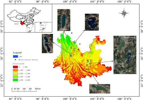
Yunnan Province, China, is characterised by nine lakes with areas larger than 10 km^2: Dianchi, Chenghai, Erhai, Lugu, Fuxian, Qilu, Yilong, Xingyun, and Yangzonghai (Wu et al. 2016). The NYPLs are located in central, southern, western, and northwestern Yunnan Province between 21°29′−29°19′ N and 97°50′−105°36′ E (see Figure 1). The study region has an elevation ranging from 6,740 m in the north-west to 76 m in the south-east, with an average elevation of approximately 2,000 m (Yang et al. 2005). This region has a distinctive monsoon climate, where the average annual temperature is approximately 15 °C, and the average annual precipitation is >1,000 mm, with a decreasing pattern from north to south (Yang et al. 2005). In Yunnan, the rainy season (May-October) and dry season (November-April) are highly evident; therefore, the rainy season accounts for approximately 90% of the annual precipitation. The NYPLs are large-scale natural freshwater lakes sensitive to regional climate and environmental changes, such that they have attracted the attention of various researchers.

Figure 1. Study region and location of the NYPLs.

2.2. Datasets

2.2.1. Landsat images

To monitor inter-annual and seasonal changes in the SWAs of the NYPLs, dense time-series 30 m Landsat images were used in our study, including Landsat 5 TM, Landsat 7 ETM+, and Landsat 8 OLI. All Landsat images representing calibrated top-of-atmosphere (TOA) reflectance data were obtained from 1 January 1988 to 31 December 2021 using the GEE platform (http://earthengine.google.com) (Pande 2022). Detailed statistical information on the Landsat series of images used in this study is presented in Table 1. High-quality satellite imagery, which is not affected by clouds and shadows, is critical for mapping the annual and seasonal SWAs of the NYPLs; therefore, low-quality satellite images resulting from ineffective pixels (such as clouds, cloud shadows, terrain shadows and snow) were first masked using Fmask on the GEE platform (Kandekar et al. 2021; Pande 2022).

Table 1. Properties of the image collections selected for this study.

Sensors	Years	Number of images
		All year	Dry season	Rainy season
Landsat 5 TM Landsat 7 ETM+ Landsat 8 OLI	1988–1997	354	212	142
	1998–2007	415	214	201
		389	197	192
	2008 − 2021	100	42	58
		349	181	158
		446	177	249

2.2.2. Auxiliary data

The auxiliary data mainly consisted of a digital elevation model (DEM), validation samples, and meteorological data. DEM data were required in this study and were used to remove terrain shadows. High-resolution global DEMs (GDEMs) were generated from publicly available Aster stereoscopic datasets. Validation samples of surface water were obtained by manual interpretation based on high spatial resolution remote sensing images from the GEE, which were used to evaluate the accuracy of surface water mapping in the NYPLs. The meteorological data used in this study were provided by Data Centre of the China Meteorological Administration (http://www. data.cma.cn/), which provided the correlation between changes in SWAs and meteorological factors. Figure 1 shows the locations of the meteorological stations closest to the nine plateau lakes.

2.3. Water indices

The spectral water index is a single value, usually derived from the reflection of two or more spectral bands or the values of related bands by some calculation, including ratio, difference, normalization, multiplication or others. Recently, various water indices based on Landsat images have been successfully used to extract inland surface water bodies (Xie et al. 2016), but different water indices have their own advantages and disadvantages. Among these, the NDWI_McFeeters (Mcfeeters 1996), MNDWI (Xu 2006), NWI (Feng 2012), AWEI (Feyisa et al. 2014) and WI₂₀₁₅(Fisher et al. 2016) can provide the best results for different geographical regions (such as urban, rural, and plateau regions). The NYPLs are located in different geographical environments such that the extraction of lake surface water is easily affected by various factors including snow, mountain shadows, building shadows, and different water qualities. Therefore, simultaneously obtaining the highest extraction accuracy for each lake using only a single WI is difficult. Hence, in this study, the NDWI_McFeeters, MNDWI, AWEI_sh, NWI, and WI₂₀₁₅ were employed to extract the SWAs of the NYPLs. The extraction accuracies of the SWAs using these water indices were compared for each lake. Finally, the optimum WI for each lake was selected to extract the annual and seasonal SWAs of the NYPLs from 1988 to 2021. Figure 2 shows a flow chart of this study. The NDWI_McFeeters, MNDWI, AWEI, NWI and WI₂₀₁₅ are introduced in detail and summarized in Table 2.

Figure 2. Flow chart of this study.

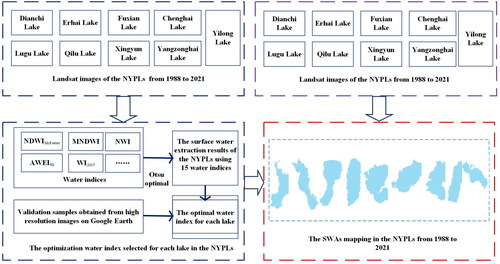
Table 2. Main water indices.

Water indices	Equations	References
NDWIMcFeeters	(ρG − ρNIR)/ (ρG + ρNIR)	(Mcfeeters 1996)
MNDWI	(DNG − DNSWIR5)/ (DNG + DNSWIR5)	(Xu 2006)
NWI	(DNB − (DNNIR + DNSWIR5 + DNSWIR7))/ (DNB + (DNNIR + DNSWIR5 + DNSWIR7))	(Feng 2012)
AWEInsh	4 * (ρG − ρSWIR5) − (0.25 * ρNIR + 2.75 * ρSWIR7)	(Feyisa et al. 2014)
AWEIsh	ρB + 2.5 * ρG − 1.5 * (ρNIR + ρSWIR5) − 0.25 * ρSWIR7	(Feyisa et al. 2014)
WI2015	1.7204 + 171 * ρG + 3 * ρR − 70 * ρNIR − 45 * ρSWIR5– 71 * ρSWIR7	(Fisher et al. 2016)

2.4. Optimum threshold algorithm: OTSU

All WI methods can be used to extract open surface water bodies by applying a simple threshold. However, choosing the optimal threshold is a major problem that have often been encountered. Generally, this threshold is determined for each WI to discriminate water from land and is usually set between −1 and 1. However, subjective selection of the threshold value may lead to an over- or under-estimation of the SWA because of the spectral heterogeneity between water and no-water regions in different geographical environments. Therefore, the optimal threshold value should be determined according to the characteristics of the WI values in different scenes (Ji et al. 2009).

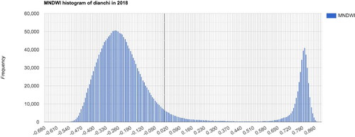
In classification methods based on threshold segmentation, it is often necessary to determine a certain threshold and separate different categories in the image, such as water and land, water and vegetation, and vegetation and soil. If a suitable threshold is obtained, a certain type of object can be completely separated. The Otsu adaptive threshold algorithm, which is a classic image segmentation methods, was proposed by Japanese scholar Otsu Nobuyuki in 1979 (Otsu 1979). This algorithm assumes that the image contains two categories of pixels according to a two-mode histogram (foreground and background pixels) and calculates the optimal threshold that can separate the two categories and minimize their inter-class variance. A constant square distance maximizes the inter-class variance of the two pairs to obtain the optimal threshold value, T, of the WI. For example, for lake Dianchi, Figure 3 shows the optimal threshold value of the MNDWI for extracting lake surface water using the Otsu algorithm in 2018, with an optimal threshold of 0.02. Previous studies have shown that the Otsu algorithm can be adopted to dynamically select the threshold value of WIs. The extraction accuracy using the Otsu algorithm is higher than that of traditional methods in which the threshold value is manually obtained (Zhang et al. 2017).

Figure 3. Optimal threshold value of the MNDI histogram for lake Dianchi in 2018.

It assumed that the optimal threshold of the WI is between a and b, where −1 ≤ a < b ≤ 1. Based on the Otsu algorithm, the threshold , T, can be divided into two categories: non-water from a to T and water from T to b. The optimal threshold value for T* in the Otsu algorithm was determined as follows: (1) $$\{\begin{array}{c}{\delta }^2=P_{nw}\times {\left({\mathrm{M}}_{nw}-M\right)}^2+P_w\times {\left({\mathrm{M}}_w-M\right)}^2\hfill \\ M=P_{nw}\times M_{nw}+P_w\times M_w\hfill \\ P_{nw}+P_w=1\hfill \\ T^{*}=\mathit{Arg}\underset{a\le T\le b}{\mathrm{Max}}\left\{P_{nm}\times {\left(M_{nw}-M\right)}^2+P_w\times {\left(M_w-M\right)}^2\right\}\hfill \end{array}$$(1) where δ is the variance between non-water and water, P_nm and P_w are the probabilities that a pixel belongs to non-water and water, respectively, M_nw and M_w are the averages of non-water and water, respectively, and M is the average of WI values.

3. Results

3.1. Accuracy assessment for surface water extraction in the NYPLs using five WIs from 1988 to 2021

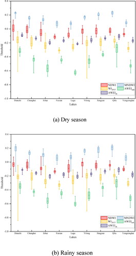
The WIs proposed in the references can suit specific geographical environments (such as rural or urban region), but it is difficult to obtain the best accuracy for each lake during different periods. Therefore, five WIs were used separately to extract the SWAs of the NYPLs at three-year intervals from 1988 to 2021.The Otsu algorithm was employed to select the optimal threshold value of each WI at different stages. Table 3 lists the optimal threshold settings. In this study, 4,000 water and 4,000 no-water testing samples were generated for each lakes in each period by manually interpreting high spatial resolution images from the GEE platform. The overall accuracy (OA) and kappa coefficient are commonly adopted as accuracy assessment indices, with which all results using the five WIs were verified during the dry and rainy seasons from 1988 to 2021. The accuracy assessment of the NYPLs using the five WIs in the dry and rainy seasons of each period is shown as box plots (Figures 4 and 5). According to the results, the extraction accuracy differed when five WIs were applied to the surface water extraction of the NYPLs in different periods; it was difficult to obtain the highest accuracy for the 9 plateau lakes in 12 periods. The five WIs obtained the highest OA and Kappa values for each lake during different periods. The MNDWI exhibited the highest accuracy for lakes Dianchi, Chenghai, Lugu, and Yilong. The extraction accuracy of the NDWI was the highest for lakes Erhai, Fuxian, and Xingyun. The extraction accuracy of the AWEI_nsh was the highest for lake Qilu. The MNDWI and AWEI_sh showed the highest accuracy for Lake Yongzonghai during the rainy and dry seasons, respectively. The OA and Kappa coefficients of all the lakes were above 90% and 0.85, respectively, from 1988 to 2021. In short, the results demonstrated that the WI method was effective for extracting SWAs from the NYPLs.

Figure 4. Kappa and OA values of the five WIs in the dry season from 1988 to 2021.

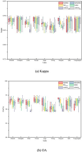
Figure 5. Kappa and OA values of the five WIs in the rainy season from 1988 to 2021.

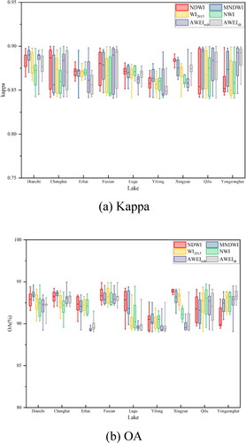
Table 3. Annual SWAs of the NYPLs from 1988 to 2021(three-year intervals).

Lakes (km^2)	Periods
	1988	1991	1994	1997	2000	2003	2006	2009	2011	2015	2018	2021
Dianchi	294.37	299.34	295.57	297.21	298.15	297.66	296.52	297.33	295.32	297.51	297.73	298.01
Fuxian	214.01	213.94	214.58	214.71	215.09	214.80	215.52	214.76	214.42	213.49	213.56	214.55
Erhai	237.49	245.07	240.44	238.30	241.81	239.84	240.75	243.30	242.55	241.63	241.62	242.15
Qilu	36.94	29.14	33.10	37.18	36.15	35.40	33.13	35.89	34.56	22.46	32.63	35.09
Yilong	33.78	28.39	29.07	29.41	31.56	30.73	26.87	30.24	27.01	13.45	27.45	28.61
Lugu	50.44	51.07	52.18	50.73	49.87	49.63	49.59	49.78	49.70	49.23	49.28	49.39
Chenghai	74.89	75.12	74.95	74.73	75.22	75.47	74.97	75.01	74.56	73.47	73.08	72.70
Xingyun	33.90	34.00	34.17	34.03	33.78	32.92	33.79	33.53	33.21	31.68	33.86	33.98
Yangzonghai	30.32	30.21	30.16	30.43	30.89	30.85	30.81	30.65	30.52	30.02	30.45	30.48

Bold values are the maximum and minimum SWAs of each lake during the period.

3.2. Spatiotemporal dynamic changes of the SWAs in the NYPLs from 1988 to 2018

3.2.1. Inter-annual changes

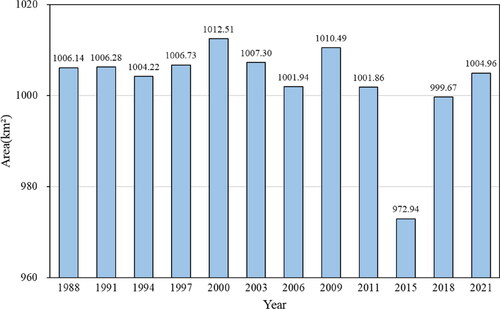
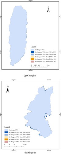
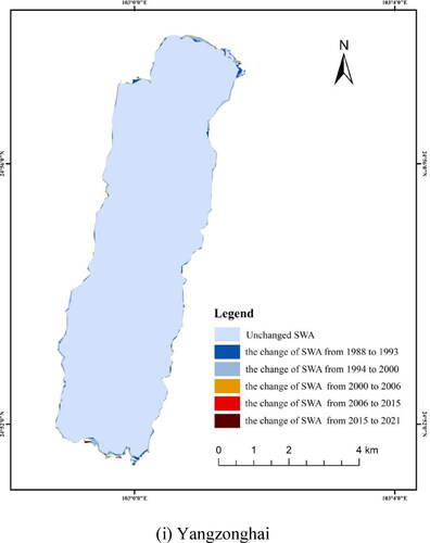
According to the accuracy assessment results in Section 3.1, we chose the best accuracy results of the NYPL SWAs from the five WIs. The annual SWAs were obtained by averaging the results of the dry and rainy seasons for each period. To illustrate the change in lake area with time, the total SWAs of the NYPLs extracted were plotted for each stage (Figure 6). Based on the overall lake analysis, the plateau lake area in the Yunnan Province had been changed significantly for more than 30 years, reaching a maximum of 1,012.51 km² in 2000. From 1988 to 2015, the overall SWAs of the nine plateau lakes fluctuated steadily within 1%. Since 2015, the total SWAs first decreased and then increased, reaching the lowest point of 972.94 km² in 2015. According to Table 3, the individual lakes changed with time. Among the three large lakes (>200km²), the SWA change was relatively stable. The SWA changes in the lakes Dianchi, Erhai, and Fuxian were with a range of less than from 1998 to 2021.However, the SWA changes of the Lakes Dianchi and Erhai were larger than those in lake Fuxian. In the six other smaller lakes (<100km²), the SWAs of Lugu, Chenghai, and Yangzonghai did not change significantly, with a change of less than 7.29% from 1998 to 2021. However, lakes Qilu and Yilong showed significant changes in the area. Lake Qilu decreased by 39.59% from 1998 to 2015, and Lake Yilong decreased by 60.18% from 1998 to 2015. The results of this study showed that the change trends of the SWAs in the NYPLs from 2000 to 2015 are consisted with the results in Wu et al. (2016).

Figure 6. Total SWAs of the NYPLs from 1988 to 2021.

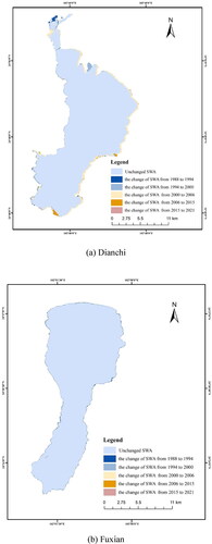
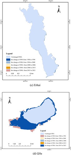
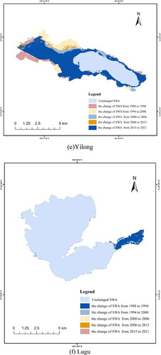
Increases and decreases in lake areas are not only reflected in time but also in space, which is closely related to the geographical location of the lake and the local climatic conditions. From the perspective of the regional geographical position, lakes Chenghai, Lugu, Fuxian, and Erhai, which are located in the high-altitude area northwest of Yunnan Province, showed little change in their area, whereas lakes Qilu and Yilong southeast of Yunnan Province, which are located at lower elevations, showed significant changes in their area. From the perspective of spatial changes, lake Dianchi, Qilu, and Yilong have undergone significant changes over the past 30 years. As shown in Figure 7, the three lakes shrank in different directions during different periods. Owing to urbanization in Kunming, shrinkage occurred around Lake Dianchi from 1988 to 2021. The main shrinkage area was to the west of lake Yilong. However, southwest of lake Qilu was the main shrinkage from 1988 to 2015. The SWAs of Lakes Yilong and Qilu have expanded since 2015.

Figure 7. Changes in the NYPLs from 1988 to 2021 (six-year intervals).

3.2.2. Seasonal changes

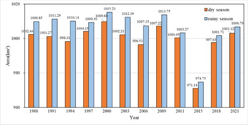
Precipitation is an important factor in SWA changes in the NYPLs. Figure 8 shows the total SWAs of the NYPLs during dry and rainy from 1988 to 2021.Generally, the SWAs in the rainy season were larger than in the dry season; however, there were some differences in each period. The SWA change was approximately 10 km² in 1991, 1994, and 2003, and the SWA change was relatively less in the other years.

Figure 8. Total SWAs of the NYPLs in rainy and dry seasons from 1988 to 2021.

According to Table 4, the SWA changes in the NYPLs in the dry and rainy seasons show that the NYPLs expanded from the dry to rainy seasons between 1988 and 2021. However, the SWAs of most lakes not excessively large. The changes in lake Dianchi were approximately 2–6 km² in 1988, 1994, 2006, 2009, and 2015, and less than 2 km² in the other years. The SWAs of lakes Fuxian, Lugu, Chenghai, Xingyun, and Yangzonghai were very stable under dry and rainy conditions from 1998 to 2021, with changes of less than 2 km². The area of lake Erhai was approximately 3 km² in 1991 and 2003, and there were no-changes in the other years. The changes in lakes Qilu and Yilong ranged from 1 to 3 km² from 1988 to 2021. In summary, the large lakes, except for lake Fuxian, had greater seasonal changes, and the seasonal changes in the shallow lakes were greater than those in the deep-water lakes.

Table 4. Annual SWAs of the NYPLs in the dry and rainy seasons from 1988 to 2021(three-years intervals).

Lakes (km^2)	Periods
	1988	1991	1994	1997	2000	2003	2006	2009	2011	2015	2018	2021
Dianchi (dry/rainy)	293.33	299.32	293.43	296.72	298.01	297.03	293.25	296.11	294.85	296.87	297.09	297.42
	295.41	299.36	297.72	297.70	298.29	298.28	299.78	298.55	295.80	298.15	298.36	298.61
Fuxian (dry/rainy)	213.82	213.76	213.73	214.51	214.90	214.54	215.05	214.40	214.10	213.39	213.07	213.81
	214.19	214.13	215.43	214.90	215.28	215.06	215.99	215.12	214.73	213.60	214.06	215.28
Erhai (dry/rainy)	237.49	243.36	240.02	238.30	241.41	238.57	240.04	243.30	242.26	241.53	241.62	242.15
	237.49	246.77	240.86	238.30	242.21	241.11	241.47	243.30	242.85	241.74	241.62	242.15
Qilu (dry/rainy)	35.32	28.95	32.32	36.76	35.57	34.49	32.69	35.50	34.52	22.30	32.51	35.34
	38.56	29.34	33.88	37.59	36.73	36.31	33.57	36.28	34.59	22.61	32.75	34.84
Yilong (dry/rainy)	33.64	27.16	28.75	28.38	31.56	30.11	26.74	29.83	26.88	13.35	26.92	28.16
	33.93	29.62	29.38	30.43	31.56	31.35	27.00	30.64	27.14	13.55	27.97	29.06
Lugu (dry/rainy)	50.22	50.22	51.42	50.61	49.46	49.35	49.56	49.62	49.80	49.09	49.24	49.31
	50.66	51.92	52.94	50.86	50.27	49.91	49.61	49.94	49.60	49.36	49.32	49.46
Chenghai (dry/rainy)	74.84	74.54	74.69	74.54	74.92	75.41	74.84	74.77	74.52	73.36	73.02	72.63
	74.93	75.69	75.22	74.92	75.53	75.52	75.09	75.24	74.61	73.58	73.14	72.76
Xingyun (dry/rainy)	33.66	33.79	34.12	33.98	33.23	32.07	33.61	33.14	33.21	31.56	33.85	33.89
	34.14	34.21	34.22	34.08	34.34	33.77	33.97	33.92	33.21	31.80	33.88	34.08
Yangzonghai (dry/rainy)	30.10	30.17	29.83	30.34	30.75	30.63	30.75	30.54	30.30	29.69	30.30	30.40
	30.54	30.25	30.50	30.53	31.03	31.07	30.87	30.76	30.75	30.36	30.60	30.56

3.3. SWAs variation in the NYPLs influenced by other factors

3.3.1. Correlation between SWAs of the NYPLs and precipitation

Figure 9 shows the correlation between the total SWAs of the NYPLs and precipitation. Over the past 30 years, the changes in the SWAs of the NYPLs were consistent with the trend in precipitation. However, it fluctuated significantly in 2015. Table 5 lists the differences in the correlation statistics between the SWA of each lake and precipitation. The SWAs of lakes Chenghai and Fuxian showed stronger positive correlations with precipitation from 1988 to 2011. The SWAs of Lake Dianchi also showed a clear positive correlation with precipitation from 2011 to 2021. In others word, precipitation was a direct factor causing SWA changes in the NYPLs.

Figure 9. Total SWAs of the NYPLs and average precipitation from 1988 to 2021.

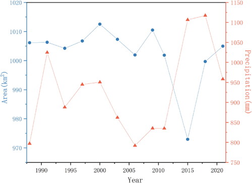
Table 5. Correlation statistic between the SWAs of the NYPLs and average precipitation from 1988 to 2021.

Lake	1988–2011		2011–2021
	R	p-value	R	p-value
Chenghai	**0.46	0.02	−0.62	0.26
Dianchi	0.14	0.47	**0.95	0.001
Erhai	0.26	0.21	0.15	0.81
Fuxian	**0.51	0.01	0.80	0.11
Lugu	0.33	0.10	0.42	0.48
Qilu	0.33	0.10	0.83	0.08
Xingyun	0.65	3.40	0.70	0.19
Yanzhonghai	0.37	0.06	0.80	0.10
Yilong	0.25	0.22	0.17	0.78

**means p-value < 0.05.

3.3.2. Correlation between SWAs of the NYPLs and temperature

Figure 10 shows the correlation between the total SWAs of the NYPLs and temperature. Over the past 30 years, SWAs changes in the NYPLs have been negatively correlated with temperature changes. Table 6 lists the differences in the correlation statistics between the SWA of each lake and temperature. The SWAs of Lakes Dianchi, e Chenghai, Lugu, and Yilong showed negative correlations with temperature from 1988 to 2021. The SWAs of Lakes Erhai, Fuxian, Qilu, and Xingyun showed less correlation with temperature from 1988 to 2021. Compared to precipitation, temperature was and indirect factor that affected the SWA changes in the NYPLs.

Figure 10. Total SWAs of the NYPLs and average temperature from1988 to 2021.

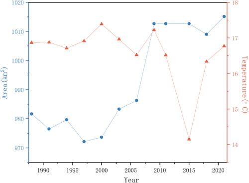
Table 6. Correlation statistics between the SWAs of the NYPLs and the average temperature from 1988 to 2021.

Lake name	1988–2021
	R	p-value
Chenghai	**−0.63	0.001
Dianchi	**−0.38	0.04
Erhai	−0.16	0.4
Fuxian	−0.08	0.68
Lugu	**−0.46	0.01
Qilu	**−0.64	0.001
Xingyun	−0.24	0.2
Yanzhonghai	−0.26	0.16
Yilong	0.05	0.79

**means p-value < 0.05.

3.3.3. Correlation between SWAs of the NYPLs and evaporation

Figure 11 shows the correlation between the total SWAs of the NYPLs and evaporation. During the past 30 years, SWA changes in the NYPLs have been negatively correlated with changes in evaporation. However, it fluctuated significantly in 2003, 2011, and 2021. Table 7 lists the differences in the correlation statistics between the SWA of each lake and evaporation. The SWAs of lakes Chenghai, Yangzhonghai, Qilu, Xingyun, and Yilong showed a negative correlation with evaporation from 1988 to 2021. The SWAs of lakes Dianchi, Erhai, Fuxian, and Lugu were less correlated with evaporation from 1988 to 2021. Evaporation had more of an influence on shallow lakes than on deep-water lakes and was another indirect factor that caused SWA changes in the NYPLs.

Figure 11. Total SWAs of the NYPLs and average evaporation from1988 to 2021.

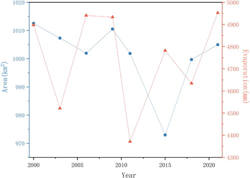
Table 7. Correlation statistics between the SWAs of the NYPLs and the average evaporation from 1988 to 2021.

	1988–2021
Lake	R	p-value
Chenghai	**−0.57	0.001
Dianchi	−0.25	0.52
Erhai	−0.24	0.36
Fuxian	−0.08	0.68
Lugu	−0.27	0.09
Qilu	**−0.53	0.002
Xingyun	**−0.37	0.003
Yanzhonghai	**−0.46	0.001
Yilong	**0.39	0.004

**means p-value < 0.05.

3.3.4. Influence of human factors

Many experimental studies have shown that human activities also affect the change in water area in the NYPLs, the most obvious being changes in land use and the influence of local policies and governance (Liu et al. 2020b).

The changes in Lake Dianchi mainly lie in the contraction in the north and the increase or decrease in the east-west direction. From 1991 to 2011, there was a small decrease in the northern Caohai area while some areas increased in an east-west direction. Meanwhile, there were different degrees of contraction in all surrounding areas, which were related to the construction of a sewage treatment plant in the Lake Dianchi Basin and a series of sludge-clearing projects. The SWAs of Lake Dianchi increased slightly since 2011. This may be related to the Niulanjiang Diversion Project completed in 2013, which diverted water from Niulanjiang River to Lake Dianchi.

Lake Yilong varied the most among the nine plateau lakes. From 1988 to 1997, a large area shrank northwest of Lake Yilong. Between 1998 and 2011, the northwest region began to expand, whereas the south-east contracted slightly. Between 2009 and 2021, the northern part of the lake contracted, and the southern part expanded. Notably Lake Yilong shrank significantly after 2011. The main reasons for the decrease in the lake area over the past 30 years are as follows. (1) Lake Yilong Basin is located in a densely populated and urbanized area, which is the source of industrial and agricultural water along the lake and irrigation water in the downstream area. (2) In the south bank area, lakes were built to cultivate crops, while fish ponds were built in the west and north to reduce the lake area.

The area of Lake Qilu increased in some years but decreased in others. From 1988 to 1997, southwestern Lake Qilu was the main contraction area. Between 1998 and 2009, Lake Qilu shrank in both the southwest and northeast. From 2009 to 2021, Lake Qilu shrank in the southwest and increased in the northeast. Notably Lake Qilu shrank significantly after 2011.The main driving factors that caused Lake Qilu to shrink in the southwest direction include the following. (1) Lake Qilu Basin is densely populated, accelerating urbanization. The levees and cofferdams encompassing the lake destroyed the natural land-water transition zone and thus reduced the size and volume of the lake basin. (2) As one of the main sources of water for life, industry, and agriculture in Tonghai County, water consumption from Lake Qilu increases annually, shaping the pattern of decreasing runoff into the lake and subsequently increasing outflow. (3) Large-scale projects, especially the construction project of Pan-Asia railway tunnel, have damaged the balance of groundwater resources in southwestern Tonghai County, leading to the exhaustion of some dams and springs, while aggravating the drought crisis of Lake Qilu.

Additionally, continuous drought in southwest China (mainly Yunnan Province) since 2011 has highlighted the superimposed effect of drought, leading to severe water shortages in most lakes in Yunnan Province, which is one of the reasons for lake area reduction after 2011.

Over the past 30 years, the land use of each lake basin in Yunnan Province has undergone significant changes. With the development of the social economy, the construction and cultivated land areas of each basin have increased annually. Owing to its location, construction land in the Lake Dianchi Basin had the fastest growth rate. Moreover, due to social and economic development, the population has increased dramatically, leading to a continuous increase of in pollutants entering the lake. Therefore, treatments face increasing difficulty in Lake Dianchi. After four years of drought in Yunnan Province since 2010, most the plateau lakes have shrunk. However, owing to the increase in the cultivated land area around Lake Yilong, land reclamation has occurred. Due to the development of tourism in lakes Erhai and Lugu, a large amount of domestic sewage discharge has deteriorated the water quality. Lake Qilu is a shallow, closed lake and a source of water for both daily life and agricultural irrigation in Tonghai County. As a result, the lakeside zone is seriously damaged; soil erosion is serious, leading to a significant reduction in the water area. The area of plateau lakes in Yunnan Province has recently decreased. Through the visual interpretation of high-resolution images, in addition to the water pollution evidenced by changes in water colour, the construction land area of each lake basin was also found to be expanding, which can best reflect the intensity of human activities.

4. Discussion

4.1. Optimal threshold selection of five WIs for the NYPLs

Optimal threshold selection is the key to the method using WI threshold segmentation, which directly affects the extraction accuracy of the SWA. Otsu’s method can automatically determine the optimal segmentation threshold and is widely used in surface water extraction in combination with WIs. However, the optimal thresholds were different for the five WIs of the NYPLs from 1988 to 2021. Figure 12 shows the selection results for the dry and rainy season. The optimal thresholds of the MNDWI, NDWI, WI_2015, AWEI_nsh, and AWEI_sh ranged from 0.1 to 0.3, −0.1 to 0.1, −0.1 to −0.3, −0.2 to −0.6, and −0.2 to 0, respectively, in the dry and rainy season. Figure 9 shows that the optimal threshold of each WI varied widely for different lakes during different periods. Therefore, the geographical environment and water quality of the NYPLs were responsible for the optimal threshold difference for each lake based on the same WI.

Figure 12. Optimal thresholds of the five WIs for the NYPLs in the dry and rainy seasons from 1988 to 2021.

4.2. Comparison with visual interpretation results

Visual interpretation (VI) was carried out using high spatial resolution remote sensing imagery from the GEE in 2021, which is the real standard data used to assess the performance of the WI methods. Figure 13 and Table 8 present qualitative and quantitative results, respectively. WI methods can easily to produce errors owing to mixed pixels at the land and water boundary. However, the best accuracy results for the WIs were quite consistent with the VI results for the YNPLs (Figure 13); the precision was 96% for the NYPLs, as listed in Table 8.

Figure 13. Comparison of the SWAs of the NYPLs extracted by the WIs and VI in 2021.

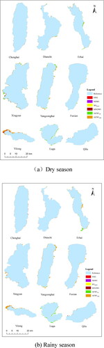
Table 8. Accuracy comparison of the SWAs of the NYPLs extracted by the WIs and VI for the image from 2021.

Lake	Best accuracy results of WIs (km^2)	VI (km^2)	Precision (%)
Dianchi (dry/rainy)	297.42/298.61	299.46/ 300.08	99.32%/99.51%
Fuxian (dry/rainy)	213.81/ 215.28	215.46/ 215.49	99.23%/99.90%
Erhai (dry/rainy)	242.15/ 242.15	245.29/246.46	98.72%/98.25%
Qilu (dry/rainy)	35.34/ 34.84	36.20/ 36.02	97.87%/96.72%
Yilong (dry/rainy)	28.16/29.06	28.77/28.92	97.88%/97.70%
Lugu (dry/rainy)	49.31/49.46	50.32/50.53	97.99%/97.88%
Chenghai (dry/rainy)	72.63/72.76	72.94/73.16	99.57%/99.45%
Xingyun (dry/rainy)	33.89/34.08	34.67/ 34.87	97.75%/97.73%
Yangzonghai (dry/rainy)	30.40/30.56	30.80/30.83	98.70%/99.12%

5. Conclusions

Based on the Landsat remote sensing images on the GEE platform, the optimal WI and best threshold were chosen through many verification experiments to extract the SWAs of the NYPLs in the dry and rainy seasons from 1988 to 2021. In this study, the high accuracy SWAs in the NYPLs were generated from 1988 to 2021. The inter-annual and dry-rainy seasonal spatiotemporal changes of the SWAs in the NYPLs were first analyzed. Meanwhile, the major driving factors that affect the inter-annual and seasonal changes in SWAs were identified, respectively. In the past three decades, the total SWAs of the NYPL have remained stable, and shown an increase-decrease-increase trend. The SWAs during the rainy season were larger than during the dry season. however, there were some differences between each period. Precipitation is a direct factor affecting SWA changes in the NYPLs, whereas temperature and evaporation are two indirect factors. The changes in the SWAs of the NYPLs were consistent with the changing trends in precipitation, and were negatively correlated with temperature and evaporation change. Evaporation has more of an influence on shallow lakes than deep-water lakes. Human activities are one of the main factors that cause the shrinkage and expansion of the NYPLs. Therefore, climatic factors and human activities are important factors affecting SWA changes in the NYPLs. This study provides a new understanding of the impacts of climate and environmental changes, human activities, and SWA variation across the NYPLs over the past 33 years. It also provides important references for researchers to monitor future changes in the NYPLs and for the government to formulate relevant protection policies. However, the proposed method need manually choose the WI and optimal threshold for each lake, it is difficult to achieve mapping of global surface water. Next work, how to develop the WI suitable for mapping the large-scale surface water in complex geographical environment.

Disclosure statement

No potential conflict of interest was reported by the authors.

Additional information

Funding

This work was funded by Major Scientific and Technological Projects of Yunnan Province (No:202202AD080010); National Natural Science Foundation of China (No:42171392); Yunnan Province Basic Research Special Key Project (No.202001AS070032); Yunnan Province Young Academic and Technical Leaders Reserve Talent Project (No.202105AC160059).

References

- Aires F, Venot J-P, Massuel S, Gratiot N, Pham-Duc B, Prigent C. 2020. Surface water evolution (2001–2017) at the Cambodia/Vietnam border in the upper mekong delta using satellite MODIS observations. Remote Sens. 12(5):800. doi: 10.3390/rs12050800.
- Arvor D, Daher FRG, Briand D, Dufour S, Rollet A-J, Simões M, Ferraz RPD. 2018. Monitoring thirty years of small water reservoirs proliferation in the southern Brazilian Amazon with Landsat time series. ISPRS J Photogramm Remote Sens. 145:225–237. doi: 10.1016/j.isprsjprs.2018.03.015.
- Chen B, Xiao X, Li X, Pan L, Doughty R, Ma J, Dong J, Qin Y, Zhao B, Wu Z, et al. 2017. A mangrove forest map of China in 2015: analysis of time series Landsat 7/8 and Sentinel-1A imagery in Google Earth Engine cloud computing platform. ISPRS J Photogramm Remote Sens. 131:104–120., doi: 10.1016/j.isprsjprs.2017.07.011.
- Duan Q, Tan M, Guo Y, Wang X, Xin L. 2019. Understanding the spatial distribution of urban forests in China using Sentinel-2 images with Google Earth Engine. Forests. 10(9):729. doi: 10.3390/f10090729.
- Feng D. 2012. A new method for fast information extraction of water bodies using remotely sensed data. Remote Sens Technol Appl. 24:167–171.
- Feyisa GL, Meilby H, Fensholt R, Proud SR. 2014. Automated Water Extraction Index: a new technique for surface water mapping using Landsat imagery. Remote Sens Environ. 140:23–35. doi: 10.1016/j.rse.2013.08.029.
- Fisher A, Flood N, Danaher T. 2016. Comparing Landsat water index methods for automated water classification in eastern Australia. Remote Sens Environ. 175:167–182. doi: 10.1016/j.rse.2015.12.055.
- Guo Y, Xia H, Zhao X, Qiao L, Du Q, Qin Y. 2022. Early-season mapping of winter wheat and garlic in Huaihe basin using Sentinel-1/2 and Landsat-7/8 imagery. IEEE J Sel Top Appl Earth Observ Remote Sens. 15:1–10. doi: 10.1109/JSTARS.2022.3215589.
- Hamunyela E, Hipondoka M, Persendt F, Sevelia Nghiyalwa H, Thomas C, Matengu K. 2022. Spatio-temporal characterization of surface water dynamics with Landsat in endorheic Cuvelai-Etosha Basin (1990–2021). ISPRS J Photogramm Remote Sens. 191:68–84. doi: 10.1016/j.isprsjprs.2022.07.007.
- Hao B, Ma M, Li S, Li Q, Hao D, Huang J, Ge Z, Yang H, Han X. 2019. Land use change and climate variation in the three gorges reservoir catchment from 2000 to 2015 based on the Google Earth Engine. Sensors. 19(9):2118. doi: 10.3390/s19092118.
- Harris A. 1994. Time series remote sensing of a climatically sensitive lake. Remote Sens Environ. 50(2):83–94. doi: 10.1016/0034-4257(94)90036-1.
- Ji L, Zhang L, Wylie BK. 2009. Analysis of dynamic thresholds for the normalized difference water index. Photogramm Eng Remote Sens. 75(11):1307–1317. doi: 10.14358/PERS.75.11.1307.
- Kandekar VU, Pande CB, Rajesh J, Atre AA, Gorantiwar SD, Kadam SA, Gavit B. 2021. Surface water dynamics analysis based on sentinel imagery and Google Earth Engine Platform: a case study of Jayakwadi dam. Sustain Water Resour Manag. 7(3):44. doi: 10.1007/s40899-021-00527-7.
- Li R, Xia H, Zhao X, Guo Y. 2023. Mapping evergreen forests using new phenology index, time series Sentinel-1/2 and Google Earth Engine. Ecol Indic. 149:110157. doi: 10.1016/j.ecolind.2023.110157.
- Liu D, Chen N, Zhang X, Wang C, Du W. 2020a. Annual large-scale urban land mapping based on Landsat time series in Google Earth Engine and OpenStreetMap data: a case study in the middle Yangtze River basin. ISPRS J Photogramm Remote Sens. 159:337–351. doi: 10.1016/j.isprsjprs.2019.11.021.
- Liu X, Shi Z, Huang G, Bo Y, Chen G. 2020b. Time series remote sensing data-based identification of the dominant factor for Inland Lake Surface Area Change: anthropogenic activities or natural events? Remote Sens. 12(4):612. doi: 10.3390/rs12040612.
- Ma S, Zhou Y, Gowda PH, Dong J, Zhang G, Kakani VG, Wagle P, Chen L, Flynn KC, Jiang W. 2019. Application of the water-related spectral reflectance indices: a review. Ecol Indic. 98:68–79. doi: 10.1016/j.ecolind.2018.10.049.
- Mcfeeters SK. 1996. The use of the Normalized Difference Water Index (NDWI) in the delineation of open water features. Int J Remote Sens. 17(7):1425–1432. doi: 10.1080/01431169608948714.
- Miao Z, Fu K, Sun H, Sun X, Yan M. 2018. Automatic water-body segmentation from high-resolution satellite images via deep networks. IEEE Geosci Remote Sens Lett. 15(4):602–606. doi: 10.1109/LGRS.2018.2794545.
- Mishra AP, Khali H, Singh S, Pande CB, Singh R, Chaurasia SK. 2021. An assessment of in-situ water quality parameters and its variation with Landsat 8 level 1 surface reflectance datasets. Int J Environ Anal Chem. 101:1–23. doi: 10.1080/03067319.2021.1954175.
- Mueller N, Lewis A, Roberts D, Ring S, Melrose R, Sixsmith J, Lymburner L, McIntyre A, Tan P, Curnow S, et al. 2016. Water observations from space: mapping surface water from 25years of Landsat imagery across Australia. Remote Sens Environ. 174:341–352. doi: 10.1016/j.rse.2015.11.003.
- Oliphant AJ, Thenkabail PS, Teluguntla P, Xiong J, Gumma MK, Congalton RG, Yadav K. 2019. Mapping cropland extent of Southeast and Northeast Asia using multi-year time-series Landsat 30-m data using a random forest classifier on the Google Earth Engine Cloud. Int J Appl Earth Obs Geoinf. 81:110–124. doi: 10.1016/j.jag.2018.11.014.
- Olthof I, Rainville T. 2022. Dynamic surface water maps of Canada from 1984 to 2019 Landsat satellite imagery. Remote Sens Environ. 279:113121. doi: 10.1016/j.rse.2022.113121.
- Orimoloye IR, Olusola AO, Belle JA, Pande CB, Ololade OO. 2022. Drought disaster monitoring and land use dynamics: identification of drought drivers using regression-based algorithms. Nat Hazards. 112(2):1085–1106. doi: 10.1007/s11069-022-05219-9.
- Otsu N. 1979. A threshold selection method from gray-level histograms. IEEE Trans Syst Man Cybern. 9(1):62–66. doi: 10.1109/TSMC.1979.4310076.
- Pan L, Xia H, Zhao X, Guo Y, Qin Y. 2021. Mapping winter crops using a phenology algorithm, time-series Sentinel-2 and Landsat-7/8 images, and Google Earth Engine. Remote Sens. 13(13):2510. doi: 10.3390/rs13132510.
- Pande CB. 2020. Sustainable watershed development planning. In: Pande CB, ed. Sustainable watershed development: a case study of semi-arid region in maharashtra state of India. Cham: Springer International Publishing; p. 57–69.
- Pande CB. 2022. Land use/land cover and change detection mapping in Rahuri watershed area (MS), India using the google earth engine and machine learning approach. Geocarto Int. 37(26):13860–13880. doi: 10.1080/10106049.2022.2086622.
- Pande CB, Kadam SA, Jayaraman R, Gorantiwar S, Shinde M. 2022. Prediction of soil chemical properties using multispectral satellite images and wavelet transforms methods. J Saudi Soc Agric Sci. 21(1):21–28. doi: 10.1016/j.jssas.2021.06.016.
- Pekel J, Cottam A, Gorelick N, Belward AS. 2016. High-resolution mapping of global surface water and its long-term changes. Nature. 540(7633):418–422. doi: 10.1038/nature20584.
- Phalke AR, Özdoğan M, Thenkabail PS, Erickson T, Gorelick N, Yadav K, Congalton RG. 2020. Mapping croplands of Europe, Middle East, Russia, and Central Asia using Landsat, Random Forest, and Google Earth Engine. ISPRS J Photogramm Remote Sens. 167:104–122. doi: 10.1016/j.isprsjprs.2020.06.022.
- Pickens AH, Hansen MC, Hancher M, Stehman SV, Tyukavina A, Potapov P, Marroquin B, Sherani Z. 2020. Mapping and sampling to characterize global inland water dynamics from 1999 to 2018 with full Landsat time-series. Remote Sens Environ. 243:111792. doi: 10.1016/j.rse.2020.111792.
- Qian X, Kun Y, Liang H. 2018. Remote sensing monitoring and temporal-spatial analysis of surface water body area changes of lakes on the Yunnan-Guizhou Plateau over the past 30 years. J Lake Sci. 30(4):1083–1096. doi: 10.18307/2018.0421.
- Ruan K, Zha Y, Zhou Z, Yang P. 2016. A modified GAC model for extracting waterline from remotely sensed imagery. J Remote Sens. 37(17):3961–3973. doi: 10.1080/01431161.2016.1207263.
- Shinde S, Pande CB, Barai VN, Gorantiwar SD, Atre AA. 2023. Flood impact and damage assessment based on the Sentitnel-1 SAR data using Google Earth Engine. In: Pande CB, Moharir KN, Singh SK, Pham QB, Elbeltagi A, eds. Climate change impacts on natural resources, ecosystems and agricultural systems. Cham: Springer International Publishing; p. 483–502.
- Tulbure MG, Broich M, Stehman SV, Kommareddy A. 2016. Surface water extent dynamics from three decades of seasonally continuous Landsat time series at subcontinental scale in a semi-arid region. Remote Sens Environ. 178:142–157. doi: 10.1016/j.rse.2016.02.034.
- Wang C, Jia M, Chen N, Wang W. 2018. Long-term surface water dynamics analysis based on landsat imagery and the Google Earth Engine platform: a case study in the middle Yangtze River Basin. Remote Sens. 10(10):1635. doi: 10.3390/rs10101635.
- Wang Y, Li Z, Zeng C, Xia G, Shen H. 2020. An urban water extraction method combining deep learning and Google Earth Engine. IEEE J Sel Top Appl Earth Observ Remote Sens. 13:769–782. doi: 10.1109/JSTARS.2020.2971783.
- Wang Y, Ma J, Xiao X, Wang X, Dai S, Zhao B. 2019. Long-term dynamic of poyang lake surface water: a mapping work based on the Google Earth Engine cloud platform. Remote Sens. 11(3):313. doi: 10.3390/rs11030313.
- White ME. 1978. Reservoir surface area from landsat imagery. Photogramm Eng Remote Sens. 44:1421–1426.
- Whitmore TJ, Brenner M, Jiang Z, Curtis JH, Moore A, Engstrom DR, Wu Y. 1997. Water quality and sediment geochemistry in lakes of Yunnan Province, Southern China. Environ Geol. 32(1):45–55. doi: 10.1007/s002540050192.
- Worden J, de Beurs KM. 2020. Surface water detection in the Caucasus. Int J Appl Earth Obs Geoinf. 91:102159. doi: 10.1016/j.jag.2020.102159.
- Work EA, Gilmer DS. 1976. Utilization of satellite data for inventorying prairie ponds and lakes. Photogramm Eng Remote Sens. 42:685–694.
- Wu P, Shen H, Cai N, Zeng C, Wu Y, Wang B, Wang Y. 2016. Spatiotemporal analysis of water area annual variations using a Landsat time series: a case study of nine plateau lakes in Yunnan province, China. Int J Remote Sens. 37(24):5826–5842. doi: 10.1080/01431161.2016.1251630.
- Xia H, Bian X, Pan L, Li R. 2023. Mapping tea plantation area using phenology algorithm, time-series Sentinel-2 and Landsat images. Int J Remote Sens. 44(9):2826–2846. doi: 10.1080/01431161.2023.2208713.
- Xia H, Zhao J, Qin Y, Yang J, Cui Y, Song H, Ma L, Jin N, Meng Q. 2019. Changes in water surface area during 1989–2017 in the Huai River Basin using Landsat Data and Google Earth Engine. Remote Sens. 11(15):1824. doi: 10.3390/rs11151824.
- Xie H, Luo X, Xu X, Pan H, Tong X. 2016. Evaluation of Landsat 8 OLI imagery for unsupervised inland water extraction. J Remote Sens. 37(8):1826–1844. doi: 10.1080/01431161.2016.1168948.
- Xu H. 2006. Modification of normalised difference water index (NDWI) to enhance open water features in remotely sensed imagery. Int J Remote Sens. 27(14):3025–3033. doi: 10.1080/01431160600589179.
- Yang Y, Liu Y, Zhou M, Zhang S, Zhan W, Sun C, Duan Y. 2015. Landsat 8 OLI image based terrestrial water extraction from heterogeneous backgrounds using a reflectance homogenization approach. Remote Sens Environ. 171:14–32. doi: 10.1016/j.rse.2015.10.005.
- Yang J, Zhang W, Feng W, Shen Y. 2005. Freshwater testate amoebae of nine Yunnan Plateau Lakes, China. J Freshwater Ecol. 20(4):743–750. doi: 10.1080/02705060.2005.9664798.
- Zhang G, Zheng G, Gao Y, Xiang Y, Lei Y, Li J. 2017. Automated water classification in the tibetan plateau using Chinese GF-1 WFV data. Photogramm Eng Remote Sens. 83(7):509–519. doi: 10.14358/PERS.83.7.509.
- Zhou Y, Dong J, Xiao X, Liu R, Zou Z, Zhao G, Ge Q. 2019. Continuous monitoring of lake dynamics on the Mongolian Plateau using all available Landsat imagery and Google Earth Engine. Sci Total Environ. 689:366–380. doi: 10.1016/j.scitotenv.2019.06.341.
- Zurqani HA, Post CJ, Mikhailova EA, Schlautman MA, Sharp JL. 2018. Geospatial analysis of land use change in the Savannah River Basin using Google Earth Engine. Int J Appl Earth Obs Geoinf. 69:175–185. doi: 10.1016/j.jag.2017.12.006.