Recognition of building shape in maps using deep graph filter neural network

Abstract

Shape is one of the core features of the buildings which are the main elements of the map. The building shape recognition is widely used in many spatial applications. Due to the irregularity of the building contour, it is still challenging for building shape recognition. Inspired by graph signal processing theory, we propose a deep graph filter neural network (DGFN) for the shape recognition of buildings in maps. First, we regard shape recognition as a combination of subjective and objective graph signal filtering process. Second, we construct a shape features extraction framework from the perspective of shape details, shape structure and shape local information. Third, DGFN model can fulfil the tasks of shape classification and shape embedding of building at the same time. Finally, multi angle experiments verify our viewpoint of shape recognition mechanism, and the comparison with similar algorithms proves the high accuracy and availability of DGFN model.

Keywords:

• Building
• shape recognition
• deep graph filter neural network
• shape classification
• shape embedding

1. Introduction

Shape is one of the core features of the buildings which are widely distributed in large and medium-sized maps (Steiniger et al. 2008; Henn et al. 2012). Building shape recognition is an important work of map cognition and also a basic step of cartographic generalization, spatial data updating and multi-source spatial-temporal data fusion (Xu et al. 2017; Yang et al. 2018; Zhou et al. 2018). Building shape recognition typically encompasses contour extraction from remote sensing images, followed by steps including shape classification. Extracting building outlines from remote sensing images is a crucial step in building shape recognition, involving the precise detection of both external and internal contours. However, it is challenging for the recognition of the building shape in practice. First, accurately extracting building instances from high-resolution satellite imagery remains a highly challenging task due to the complex and heterogeneous nature of building appearances in mixed backgrounds (Guo et al. 2022). Second, it is difficult to describe the shape accurately due to the irregularity of the building contour. Third, the subjective uncertainty of human beings in shape recognition also increases the difficulty.

To resolve these challenges, researchers have carried out a lot of studies. Wang H et al. (2005) used chain codes and shape numbers to describe shapes. An et al. (2011) combined chord length functions and centre distance functions to describe the multi-scale geometric features of spatial data. Tianyuan et al. (2020) used the Fourier descriptor operator of contour curves to describe shapes. Zhao et al. (2018) proposed a method that combines Mask R-CNN with boundary regularization to create regularized polygons for buildings. Liu et al. (2019) combined spatial pyramid pooling with an encoder-decoder structure to achieve automatic building segmentation from high-resolution remote sensing images. Wang S et al. (2020) introduced a novel network called Efficient Non-Local Residual U-Net (ENRU-Net), which offers superior accuracy compared to semantic segmentation models like FCN-8s and U-Net. Liu developed a multi-scale convolutional neural network framework for the extraction of building instances (Liu et al. 2021). Wei et al. (2023) proposed an end-to-end learnable framework called BuildMapper for architectural contour extraction. These studies have enriched the applications of shape recognition.

To address the subjective uncertainties in the shape recognition, researchers have expressed the subjective and objective consistency of shape recognition through template classification and matching. For example, Hao et al. used the weighted average method to calculate the spatial matching degree (Tang et al. 2008). Tong et al. proposed a matching method based on probability theory (Xiaohua et al. 2007), which determined the matching entity by calculating the entity matching probability. Yan et al. (2016) used morphological abstraction to describe the shape of buildings and constructed buildings shape template for the shape recognition and simplification. These methods work well in some typical scenarios. But most of them lack theoretical rigour and application universality in that the parameters such as features, weights, thresholds used in similarity calculation are often set by experience.

In recent years, the development of deep learning, especially convolution neural network (CNN), has opened up a broad space for computer vision and natural language processing research. CNN can extract the image features automatically through an end-to-end way and construct the nonlinear relationship between the extracted features and the results (Kim 2014; Shelhamer et al. 2017). Inspired by CNN, some researchers transform vector data into raster images and make meaningful exploration on shape recognition. In the work of Haiwei et al. (2018) and Li et al. (2020), the vector format overpass data in the city is transformed into grid format graphics, and the fuzzy features of road intersections are extracted by CNN, so as to identify the shape category of complex intersections. However, because the shape of the buildings is described by irregular vector data, when applying CNN to extract features of the buildings, some information contained in the data will be lost in the process of vector-raster conversion.

In order to address the issue of non-Euclidean data convolution, researchers have proposed graph convolutional neural networks and started applying them to shape recognition (Bruna et al. 2013).Yan et al. used graph convolution neural network to analyse the pattern of building groups (Zonghan et al. 2020). It mainly uses graph Fourier transform and convolution theorem to transform the convolution of vertex domain into the dot product of spectral domain, extracts the graph features of building groups and then predicts the types (regular and irregular) of the building groups. To code the shape of buildings, they have further proposed a graph convolutional autoencoder (GCAE) model (Yan et al. 2021). Shi et al. obtained outstanding outcomes in the extraction of building footprints by creating an innovative semantic segmentation framework that integrates Deep Structured Feature Embedding (DSFE) with GCN (Shi et al. 2020). These works have provided a meaningful exploration for the application of GNN in building shape recognition, but they have not yet revealed the complete mechanism of shape recognition. Future trends in deep learning models involve ongoing increases in model sizes and complexity, with a simultaneous focus on enhancing model interpretability and accuracy. At the same time, the application of relevant algorithms has greatly improved recognition accuracy and efficiency in building shape recognition. However, it has also introduced complex model structures and a large number of parameters. The primary challenge lies in compressing model size, enhancing processing speed and maintaining recognition accuracy. This is vital for enhancing the practicality of deep learning-based approaches.

Unlike the spectral method and the spatial method, topology adaptive graph convolutional neural (TAGCN) network is a kind of graph convolutional neural network (Velikovi et al. 2017) which is based on algebraic signal processing (ASP) theory (Sandryhaila and Moura 2013; Ortega et al. 2018). The convolution operation of TAGCN is constructed from the perspective of signal filtering, possessing both the theoretical self-consistency akin to spectral methods and the simplicity and efficiency reminiscent of spatial methods. Moreover, the concept of graph signals filtering is consistent with our point of view for the pattern of shape recognition, which is a multi-level nonlinear graph signal filtering process. Based on these factors, we build a deep graph filter neural network (DGFN) model based on the graph representation and classification ability of TAGCN network for the shape recognition of buildings. The model views the extraction of building outlines and shape classification as a comprehensive and cooperative procedure, rather than mere isolated boundary extraction. It also provides a fresh perspective on shape recognition by treating it as a combination of subjective and objective graph signal filtering, the model not only accomplishes shape embedding and shape classification together but also broadens the applicability of the model.

2. Topology adaptive graph convolutional neural filter

Graph convolution neural network is generally used for node classification, edge classification and graph classification. To achieve these goals, it is necessary to extract and aggregate multi-level graph information according to graph structure, node attributes and edge attributes. Convolution can be considered as a form of filtering, whose purpose is to enhance the signals that we want to obtain and suppress the signals that we do not want (Krizhevsky et al. 2017). The difference is that the signals of graph are the attributes of the nodes and the edges.

The advantage of traditional CNN lies in the convolution kernel with parameter sharing and local feature extracting ability. However, due to the uncertainty of the node connection number and the graph topology, it is impossible to directly apply convolution kernel with fixed size to graph data. TAGCN filter strictly defines the graph convolution operation to the graph vertex domain through the polynomial multi-plication of adjacency matrix, which is consistent with the convolution concept in traditional image signal processing. According to graph signal processing theory (Sandryhaila and Moura 2013), polynomial function of adjacency matrix can be used as graph filter. This theory extends filtering operation from traditional sequential signal processing to graph signal processing, which is also the reason why TAGCN filter has a solid theoretical foundation.

In order to construct graph convolution neural network from the idea of filtering, the graph filter should be defined first. The definition of graph filter is based on the idea of discrete signal processing (DSP)(Sandryhaila and Moura 2013). In the following, the concept of graph filter will be discussed from the concept of graph and signal on graph.

2.1. From signal filtering to graph filtering

2.1.1. Graph and signals on graph

A graph can be expressed as $G=(V,A,E),$ where $V=\{v_0,\mathrm{ }{v}_1\dots ,\mathrm{ }{v}_n\}$ is the set of the vertices of a graph, $E=\left\{\left(v_{i,j}{v}_i,v_i\in V\right)\right\}$ is the set of the edges of a graph, and $A$ is the weighted adjacency matrix. Vertex $v_i$ can represent an individual in social network or an object in spatial data, item $A_{i,\mathrm{ }j}$ in adjacency matrix denotes the connection and weight from vertex $v_j$ to vertex $v_i.$ The neighbourhood of $v_i$ can be defined as $N_i=\left\{j{A}_{i,j}\ne 0\right\}.$

The signal on a graph represents the information contained in the vertices or the edges of a graph. Let $\mathrm{X}$ be the signal, then $\mathrm{X}$ is the mapping from vertex field $\mathrm{V}$ to complex field C, and the attribute of $v_n$ can be expressed as $x_n:$ (1) $$\begin{array}{c}\mathrm{X}\text{:}\mathrm{V}\mathrm{\to }\mathrm{C}{v}_n\to x_n\end{array}$$(1)

2.1.2. From time shift to graph shift

In the field of traditional discrete signal processing (DSP), filters are used to process information. The filter takes one kind of signal as the input and produces another kind of signal as the output. Based on this idea, a linear and shift invariant graph filter can be established by analogy with linear and time invariant filter in sequential discrete signal processing.

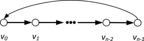
The simplest time shift filter in traditional discrete signal processing is: $x=z^{-1},$ which delays the input signal s by one time slot, so the output signal of the n-th time slot is ${\tilde{s}}_n= s_{n-1 \mathit{mod} N}.$ The directed cyclic graph shown in Figure 1 represents a finite, periodic and discrete time series, which is similar with the structure of the computation graph of building shape. All edges with the weights of 1 are directed, which reflects the causality of time series. The edge from $v_{n-1}$ to $v_0$ represents its periodicity. Its adjacency matrix A is $N\times N$ cyclic matrix $C_N,$ which is (2) $$\begin{array}{c}{A}_{n,m}=\{\begin{array}{c}1,\mathit{\text{ if n}}-m=1 \mathit{mod} N\\ 0, \mathit{otherwise} \end{array}\end{array}$$(2)

Figure 1. One dimensional periodic directed cyclic graph.

For the signal $s$ in time series, the time shift operation can be written as (3) $$\begin{array}{c}\tilde{s}=As=C_{N}s\end{array}$$(3)

In graph discrete signal processing, the concept of formula (3) is extended to general graph signals. The relationship of vertices in these graphs depends on any graph representation $G=(V,A,E).$ The operation in formula (3)(3) $$\begin{array}{c}\tilde{s}=As=C_{N}s\end{array}$$(3) is called graph shift, which replaces the signal $x_n$ of the node $v_n$ by weighted signal aggregation of its adjacent vertices. (4) $$\begin{array}{c}\tilde{s}=As{\tilde{x}}_n=\sum _{m=0}^{N-1}{A}_{n,m}{x}_m=\sum _{m\in N_n}{A}_{n,m}{x}_m \end{array}$$(4)

So the attribute of ${\tilde{x}}_n$ is the weighted sum of all adjacent vertex attributes, and the weight is that of the corresponding edge.

2.1.3. Graph filter

Similar to the traditional discrete time signal processing, a filter can be implemented by matrix multiplication on a graph. For arbitrary graph filter $\mathrm{ }\mathrm{H}\in C^{N\times N},$ a linear filtering system can be generated by multiplying the input $\mathrm{x}\in X$ with H. Here, the linear and shift invariant graph filter is studied. As shown in the formula (5)(5) $$\begin{array}{c}H\left(\alpha {\mathrm{x}}_1+\beta {\mathrm{x}}_2\right)=\alpha H{\mathrm{x}}_1+\beta H{\mathrm{x}}_2\end{array}$$(5) , the so-called linearity means that the filter for the linear combination signal is equal to the linear combination of each signal. And the graph shift invariance means that the filtering of output by graph filter is equal to the filtering of signal before processing (ie the formula (6))(6) $$\begin{array}{c}A\left(\mathrm{Hx}\right)=H\left(Ax\right)\end{array}$$(6) . (5) $$\begin{array}{c}H\left(\alpha {\mathrm{x}}_1+\beta {\mathrm{x}}_2\right)=\alpha H{\mathrm{x}}_1+\beta H{\mathrm{x}}_2\end{array}$$(5) (6) $$\begin{array}{c}A\left(\mathrm{Hx}\right)=H\left(Ax\right)\end{array}$$(6)

According to the theorem proposed in the work of Moura et al.(Sandryhaila and Moura 2013), all linear and shift invariant graph filters are polynomial functions of graph shift matrix $A.$ So the graph filter $\mathrm{H}$ can be expressed as: (7) $$\begin{array}{c}H=h\left(\mathrm{A}\right)=h_{0}I+h_{1}A+\dots +h_L{\mathrm{A}}^L\end{array}$$(7) where $h_L$ is the filter tap.

2.2. The construction of TAGCN operator

2.2.1. The definition of TAGCN filter

Without losing generality, we define the graph filter at the $l\text{-}th$ hidden layer. In the $l\text{-}th$ hidden layer, each vertex has $C_l$ attributes. The input attributes of all vertices in the $l\text{-}th$ hidden layer are defined as vector $X_c^{(l)}$($X_c^{(l)}\in R^{N_l}$), where $c=1,2\dots C_l,$ $N_l$ is the number of the vertices, and $G_{c,f}^{(l)}\in R^{N_l\times N_l}$ represents the kernel of the $f\text{-}th$ graph filter in the $l\text{-}th$ hidden layer. Then, the operation of graph filter is a matrix dot product ${G_{c,f}^{(l)}X}_c^{(l)},$ and the filtered attributes of $l\text{-}th$ layer is (8) $$\begin{array}{c}{\mathrm{ }y}_f^{\left(l\right)}=\sum _{c=1}^{C_l}{G}_{c,f}^{\left(l\right)}{X}_c^{\left(l\right)}+b_f{1}_{N_l}\end{array}$$(8)

The remainder After the activation by relu function, the $X_f^{(l+1)}$ is obtained as follows: (9) $$\begin{array}{c}{X}_f^{\left(l+1\right)}=\sigma \left(y_f^{\left(l\right)}\right)\end{array}$$(9) where $b_f^{(l)}$ is a learnable bias, and $1_{N_l}$ is a $N_l$ dimension all-1 matrix.

Graph shift matrix $A$ extends the concept of time shift from time discrete signal processing to graph structured data. From formula (7)(7) $$\begin{array}{c}H=h\left(\mathrm{A}\right)=h_{0}I+h_{1}A+\dots +h_L{\mathrm{A}}^L\end{array}$$(7) , graph filter $G_{c,f}^{\left(l\right)}$ is a polynomial of graph shift matrix $A,$ which can be expressed as: (10) $$\begin{array}{c}{G}_{c,f}^{\left(l\right)}=\sum _{k=0}^K{g}_{c,f,k}^{\left(l\right)}{A}^{k\mathrm{ }}\end{array}$$(10) where $g_{c,f,k}^{(l)}\mathrm{ }$ is the filter parameter, and k is the filter size.

2.2.2. The design of TAGCN filter

Traditional CNN scans regular grid through $K\times K\times C_l$ convolution kernel for feature extraction. For image classification task, K varies according to different CNN structures. For example, vgg-16 CNN model (Kim 2014) only uses $3\times 3\times C_l$ convolution kernel, but GoogleNet (Szegedy et al. 2015) has used several convolution kernels with different size such as $1\times 1\times C_l,$ $3\times 3\times C_l$ and $5\times 5\times C_l.$ From the perspective of information extraction, these convolutions are feature extractor, not just an embedded aggregation of attributes information. This recognition will help us better understand CNN design and apply it to irregular graph data. Similarly, we will design a general k-order neighbour filter for graph convolution neural network by defining path weight and filter size. In this graph convolution architecture, a group of filters with different size will act on the same convolution layer to extract information.

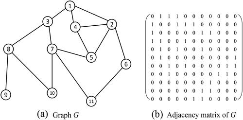
The path with the length of m on graph G is defined as a sequence of vertices $v=(v_0, v_1\dots , v_m),$ where $v_k\in V.$ Every step in the path $(v_k, v_{k+1})$ is an edge in a graph where $(v_k, v_{k+1})\in E.$ For a digraph, a path may pass through the same vertex or edge many times. Let’s take Figure 2 as an example to illustrate these concepts. The topological structure of graph G is shown on the left side of Figure 2, and the right side is the adjacency matrix of the graph. Graph G is an undirected graph, so matrix $A$ is a symmetric matrix. In this example, there are two paths with length of 2 from vertex $v_5$ to vertex $v_1,$ which are (5,4,1) and (5,2,1).

Figure 2. The example graph and its adjacency matrix.

Furthermore, the path weight is defined as the product of the weights of all edges on the path, namely, $\mathrm{\varnothing }\left(p_{0,m}\right)={\prod }_{k=1}^m{A}_{v_{k-1},v_k},$ where $p_{0,m}=\left(v_0,v_1,\dots v_m\right).$ Next, we use $\mathrm{\omega }\left(p_{j,i}^k\right)$ to denote the $\mathrm{(}\text{i, j}\mathrm{)}\text{-}th$ term of $A^k,$ then the sum of the weights of all paths with length of $k$ from $v_j$ to $v_i$ is: (11) $$\mathrm{ }\begin{array}{c}\omega \left(p_{j,i}^k\right)=\sum _{j\in \left\{\tilde{j}|\tilde{j}\mathrm{ }is\mathrm{ }k\mathrm{ }\mathit{paths}\mathrm{ }to\mathrm{ }i\right\}}\mathrm{\varnothing }\left(p_{j,i}\right)\end{array}$$(11)

It can be seen from the above example that the sum of the weights of paths (5,4,1) and (5,2,1) is $A_{5,1}^2=2.$ Combined with the formula (1)(1) $$\begin{array}{c}\mathrm{X}\text{:}\mathrm{V}\mathrm{\to }\mathrm{C}{v}_n\to x_n\end{array}$$(1) , we can get: (12) $$\begin{array}{c}{y}_f^{\left(l\right)}\left(i\right)=\sum _{k=0}^{K_l}\sum _{c=1}^{C_l}{g}_{c,f,k}^{\left(l\right)}\mathrm{\omega }\left(p_{j,i}^k\right)X_c^{\left(l\right)}\left(j\right)+b_f{1}_{N_l}\end{array}$$(12)

The above formula shows that each neuron in the graph convolution operator is only connected to the local vertex connected with it, which is adaptive to the topological structure of the graph, and the connection strength of vertices is determined by the path weight. Due to the potentially irregular topological structures of buildings in graphs, analysing the local structures and features of buildings connected only to their adjacent vertices is advantageous. This approach is not influenced by the overall graph topology, allowing the model to adapt to various shapes of buildings. To some extent, this reduces computational complexity and enhances the model’s operational efficiency, which is crucial for handling large-scale building shape data.

2.2.3. The feature extraction process of TAGCN filter

To explain the feature extraction process of graph filter, we take Figure 3 as an example. For simplicity, let $\widetilde{x_f^{\left(l\right)}}\left(i\right)$ be the convolution of vertex $v_i,$ then: (13) $$\begin{array}{c}\widetilde{x_f^{\left(l\right)}}\left(i\right)=\sum _{k=0}^{K_l}\sum _{c=1}^{C_l}{g}_{c,f,k}^{\left(l\right)}\mathrm{\omega }\left(p_{j,i}^k\right)X_c^{\left(l\right)}\left(j\right)\end{array}$$(13)

Figure 3. Information extraction process of graph filters with different sizes.

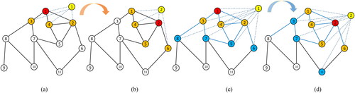
Figure 3(a,b) shows the feature extraction process of the one-order filter. When the size of the filter k = 1, the one-hop neighbours of $v_1$ is $v_2\mathrm{、}{v}_3\mathrm{、}{v}_4.$ Then, for $v_1,$ the convolution sum of k = 0 and k = 1 should be calculated in the first order convolution. After substituting the value of k, we get (14) $$\begin{array}{c}\widetilde{x_f^{\left(l\right)}}\left(1\right)=\sum _{c=1}^{C_l}\left(g_{c,f,0}^{\left(l\right)}\omega \right(p_{1,1}^0)X_c^{\left(l\right)}\left(1\right)+g_{c,f,1}^{\left(l\right)}\omega \left(p_{2,1}^1\right)X_c^{\left(l\right)}\left(2\right)\\ \hspace{1em}\hspace{1em}+g_{c,f,1}^{\left(l\right)}\omega \left(p_{3,1}^1\right)X_c^{\left(l\right)}\left(3\right)+g_{c,f,1}^{\left(l\right)}\omega \left(p_{4,1}^1\right)X_c^{\left(l\right)}\left(4\right)\end{array}$$(14)

Since the weights of the one-hop paths from these vertices to $v_1$ are all 1, $\mathrm{\omega }\left(p_{2,1}^1\right)=\mathrm{\omega }\left(p_{3,1}^1\right)=\mathrm{\omega }\left(p_{4,1}^1\right)=1.$ When setting $\mathrm{\omega }\left(p_{1,1}^0\right)=1,$ the result is as follows: (15) $$\begin{array}{c}\widetilde{x_f^{\left(l\right)}}\left(1\right)={\sum _{c=1}^{C_l}{(g}_{c,f,0}^{\left(l\right)}x}_c^{\left(l\right)}\left(1\right)+{g_{c,f,1}^{\left(l\right)}x}_c^{\left(l\right)}\left(2\right)+{g_{c,f,1}^{\left(l\right)}x}_c^{\left(l\right)}\left(3\right)+{g_{c,f,1}^{\left(l\right)}x}_c^{\left(l\right)}\left(4\right)\end{array}$$(15) where $g_{c,f,0}^{\left(l\right)}、g_{c,f,1}^{\left(l\right)}$ are the parameters of the $l\text{-}th$ hidden layer which need to be learned.

When the current vertex is transferred to $v_2,$ its one-hop neighbours are $v_1,v_4,v_5 \mathit{and} v_6.$ The convolution of vertex $v_2$ is similar to that of $v_1:$ (16) $$\begin{array}{c}\widetilde{x_f^{\left(l\right)}}\left(2\right)={\sum _{c=1}^{C_l}{(g}_{c,\mathrm{f},0}^{\left(l\right)}x}_c^{\left(l\right)}\left(2\right)+{g_{c,f,1}^{\left(l\right)}x}_c^{\left(l\right)}\left(1\right)+{g_{c,f,1}^{\left(l\right)}x}_c^{\left(l\right)}\left(4\right)+{g_{c,f,1}^{\left(l\right)}x}_c^{\left(l\right)}\left(5\right) \end{array}$$(16)

As shown in Figure 3(c,d), when the filter size becomes k = 2, for vertex $v_1,$ the one-hop neighbours are $v_2, v_3, v_4,$ and the two-hop neighbours are $v_5, v_6, v_7 \mathit{and} v_8.$ From previous analysis, we can see that the length of path $A_{5,1}^2=2,$ and the length of path $A_{6,1}^2, A_{7,1}^2, A_{8,1}^2$ are all 1, then (17) $$\begin{array}{c}\widetilde{x_f^{\left(l\right)}}\left(1\right)={\sum _{c=1}^{C_l}{(g}_{c,f,0}^{\left(l\right)}x}_c^{\left(l\right)}\left(1\right)+{g_{c,f,1}^{\left(l\right)}x}_c^{\left(l\right)}\left(2\right)+{g_{c,f,1}^{\left(l\right)}x}_c^{\left(l\right)}\left(3\right)+{g_{c,f,1}^{\left(l\right)}x}_c^{\left(l\right)}\left(4\right)\\ +{2g_{c,f,2}^{\left(l\right)}x}_c^{\left(l\right)}\left(5\right)+{g_{c,f,2}^{\left(l\right)}x}_c^{\left(l\right)}\left(6\right)+{g_{c,f,2}^{\left(l\right)}x}_c^{\left(l\right)}\left(7\right)+{g_{c,f,2}^{\left(l\right)}x}_c^{\left(l\right)}\left(8\right))\end{array}$$(17)

When the current vertex is transferred to $v_2,$ the one-hop neighbours are $v_1, v_4,v_5 \mathit{and} v_6,$ and the two-hop neighbours are $v_3, v_7, v_{11}.$ The filtering result of $v_2$ is as follows: (18) $$\begin{array}{c}\widetilde{x_f^{\left(l\right)}}\left(2\right)={\sum _{c=1}^{C_l}{(g}_{c,f,0}^{\left(l\right)}x}_c^{\left(l\right)}\left(1\right)+{g_{c,f,1}^{\left(l\right)}x}_c^{\left(l\right)}\left(2\right)+{g_{c,f,1}^{\left(l\right)}x}_c^{\left(l\right)}\left(3\right)+{g_{c,f,1}^{\left(l\right)}x}_c^{\left(l\right)}\left(4\right)\\ +{g_{c,f,2}^{\left(l\right)}x}_c^{\left(l\right)}\left(3\right)+{g_{c,f,2}^{\left(l\right)}x}_c^{\left(l\right)}\left(7\right)+{g_{c,f,2}^{\left(l\right)}x}_c^{\left(l\right)}\left(11\right))\end{array}$$(18)

3. Deep graph filter neural network for building shape recognition

3.1. The framework of DGFN model

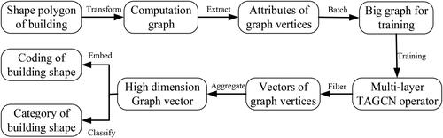
Based on the definition of the computation graph and the extraction of the shape information of the buildings, the framework of DGFN model for building shape recognition is shown as Figure 4, which consists of 5 modules. The modules are described as follows.

Figure 4. The framework of DGFN model.

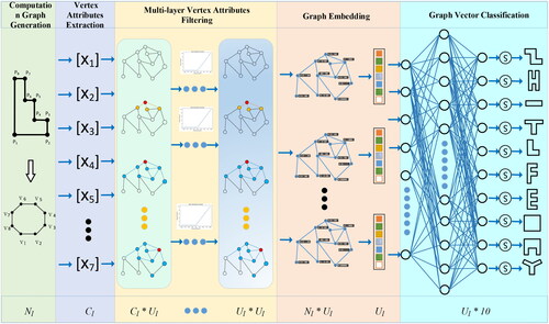
1. Computation graph generation module: This module converts the shape polygon of building to computation graph. The input is the shape polygon, and the output is a computation graph with N_l vertices.

2. Vertex attributes extraction module: It extracts and normalizes the shape details, shape structure and shape local information. The input of this module is the geometric information of shape polygon, and the output is C_l normalized attributes.

3. Multi-layer vertex attributes filtering module: It realizes multi-layer filtering and transmission of vertex attributes information. The input of this module is the adjacency matrix of computation graph and attributes of vertices, which are matrix A and N_l *C_l attributes. The first hidden layer of TAGCN operator receives these inputs. After filtering, the U_l-dimensional vertex attributes are output. Then, the multilayer TAGCN operators are connected sequentially.

4. Graph embedding module: The multi-layer filtered vertex attributes output by the last TAGCN operator is used as the embedding vector of the vertex information, which is N_l *U_l. Graph embedding module embeds vertex attribute vectors and network structure information into a graph vector. The input of this module is the N_l *U_l attributes vectors, and the output is the aggregated U_l -dimensional graph vector.

5. Graph vector classification module: The graph vector is classified by fully connected neural network and Softmax function to realize the shape classification of buildings. The input of this module is a U_l-dimensional graph vector, and the output is the probabilities that the building belongs to the different shape categories.

3.2. Conceptual model of building shape recognition with graph filters

3.2.1. Understandings of the shape recognition mechanism

Shape recognition is an instinct of human beings (Mark et al. 1999). Although there have been a lot of studies, the essence of shape recognition has not been clearly addressed. For the shape recognition mechanism, we have the following three basic understandings.

• First, the information source of shape recognition comes from the contour attributes of the spatial object. Both the artificial algorithms and human recognition must start from this point.

• Second, shape is a relative value, and the shape recognition arises from the comparison, ie comparing one shape with the obtained mental shape or with other objects.

• Third, shape recognition is a complex physiological and psychological process. The relationship between contour attributes and shape recognition is not simple linear relationship. Failure to recognize this point is the reason for the poor accuracy and low applicability of traditional methods.

From the first understanding, we can learn that the contour attributes are the input of shape recognition model. The details of contour attributes will affect the efficiency and accuracy of shape recognition. From the second understanding, we can conclude that the similarity computation, and the matching and classification of spatial objects are the concrete forms of shape recognition. From the third understanding and the principles of TAGCN graph filter, we can learn that the nonlinear relationship between contour attributes and shape recognition can be expressed by multi-layer graph signal filtering.

3.2.2. Getting shape embedding from shape classification model

Shape recognition can be achieved through two kinds of comparisons. One is shape classification when comparing with abstract shape categories. The other is shape matching when comparing with concrete object. In these recognition processes, the calculation of shape similarity is a key step. The general method to obtain shape similarity is to embed shape features into a high dimension vector, which is called shape embedding.

Shape classification and shape embedding often adopt different methods, such as self-autoencoder for graph embedding in the work of Yan et al. (2021). But different from the image autoencoder, the graph autoencoder only recovers the graph structure and cannot generate the attributes of the vertex or edge of the graph (Kipf and Welling 2016). There is still the possibility of losing the graph information when using the self-autoencoder to embed the graph. Shape classification model can realize end-to-end shape category judgement, but it can’t directly generate the embedding vector of single building shape, which limits the model’s ability to recognize the partial labelled or no labelled spatial data.

Since the shape classification model will also extract the shape information of buildings, aggregate it into a high dimension vector (usually the input vector of the fully connected layers) and recognize the shape according to the vector, it can be considered that the shape information has been aggregated into the high-dimensional vector. Then this high-dimensional vector can also be used as the embedding vector of building shape. In this way, we can use a single model to realize the function of classification and embedding at the same time. So, there will be two patterns in DGFN model, which is shape classification pattern and shape embedding pattern.

3.2.3. Conceptual model of building shape recognition with graph filters

Inspired by the understandings of shape recognition, the basic conceptual model of building shape recognition with graph filters is as follows. First, it should include some steps such as shape features extraction, multi-layer graph signal filtering and shape comparisons. Second, a computation graph should be generated from shape contour polygon according to the application rules of TAGCN graph filter. Third, there should be two patterns of the model: shape classification and shape embedding. According to these considerations, the flow chart of the conceptual model is shown in Figure 5. The detailed steps are as follows.

Figure 5. Conceptual model of building shape recognition with graph filters.

1. According to the geometric shape polygon of the building contour, the computation graph is generated;

2. Extracting the shape information of building and assign it to the corresponding vertices of the graph as its attributes;

3. Because the number of vertices of each computation graph is not the same, the batch method is used to form a large training graph with the same number of vertices;

4. The computation graph and vertex attributes are input into the model, through multi-layer information transmission and filtering to obtain the high dimension vector representation of the vertices;

5. After multi-layers of filtering, a high dimension graph vector which represents the information of the whole graph is generated from the aggregation of vertices vectors;

6. The high-dimensional graph vectors are classified into 10 categories through fully connected neural network and Softmax function.

7. The high-dimensional graph vector is obtained after the model converges, which is taken as the coding of the shape of the building and will be used to analyse the individual shape similarity.

3.3. Expressing the shape of buildings with computation graph

It is necessary to describe the objects as the form of graph in the application of graph convolution neural network. For map elements such as buildings and roads, they have the graph structure of nature. The building shape polygon can be directly used as the computation graph (Yan et al. 2021). However, there are two shortcomings in doing so. The first is the lack of attribute information and physical meaning for the nodes of the polygon. For building object, the nodes represent the intersection of the sides of shape polygon (the sides of polygon can also be called edges; to avoid confusion with the edges of the computation graph, we use the name of side here). They are not meaningful spatial objects and have little attributes. Using them as the vertexes of computation graph will probably violate the construction principle of graph convolution neural network. The second is the universality of attributes extraction. For road data, the first and last nodes are only attached to one side, while other nodes are attached with two sides at least. Therefore, there is a natural asymmetry when extracting attributes among nodes.

In addition, the process of transforming spatial objects into computation graphs can be regarded as the process of recognition and expression of spatial objects. Different from taking the natural shape polygon of building as the computation graph, we will use equivalent computation graph from another perspective. For the computation graph, its vertex represents the side of the shape polygon, and its edge represents the connection relationship of the sides. This is to say, the side of shape polygon is the basic unit in the shape recognition process in our model. In this way, a road can be regarded as an orderly connection of a series of sides, while a building is a closed-loop connection of orderly sides.

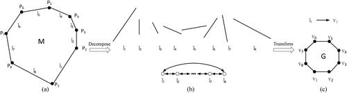
According to this understanding, as shown in Figure 6, the building shape polygon M is defined by the sides list $\mathrm{ }\mathrm{L}\left(l_1{,l}_2,l_3\dots ,l_8\right).$ And there is a node set $\mathrm{P}\left(p_1{,p}_2,p_3\dots ,p_8\right)$ which are connected with the sides. We decompose M into sides as shown in Figure 6(b). The order of sides represents the connection relationship of the graph. Then, we transform the sides into the vertices of the computation graph and transform the connection relationship between sides into the edges between the vertices of the computation graph. Finally, we form the equivalent computation graph G as shown in Figure 6(c). Vertex set $\mathrm{V}\left(v_1, v_2,v_3\dots {,v}_8\right)$ in graph G represents a series of sides, and the edge $(v_{1 }{v}_2)$ represents the connection relationship of the sides $l_1{、l}_2$ in the original shape polygon M. Since the edge of the computation graph only represents the connection relationship, its length and orientation are independent of the shape of the building. Therefore, we only need to consider the attributes and the connection relationship of the vertices in graph G.

Figure 6. Flow chart of the computation graph generation (a) shape polygon M of building (b) decomposition M to sides (c) transformation the side into the vertex.

3.4. Extraction and expression of building shape information

After the transformation from the shape polygon of building to the computation graph, the attributes of the vertexes of the computation graph need to be extracted to express the building shape. The most intuitive information of a vertexes comes from the side that it represents in the original shape polygon. In the task of shape coding and expression, there is no unified standard for shape information extraction. Because the target is shape recognition, we do not consider the position of the building.

3.4.1. Detail information of building shape

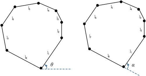
The shape polygon of building is composed of sides connected from head to tail. A single side can be reproduced by length and orientation attributes. Therefore, we select the length and orientation as the attributes of the side. The length is expressed by the Euclidean distance l between the two end points. There are two expressions of orientation, namely azimuth angle and turning angle, as shown in Figure 7. Azimuth angle θ can be defined as the angle between the side and the horizontal or vertical orientation, which is the objective value. Turning angle α is the deflection angle of the current side relative to the previous one, which is relative to the shape polygon of building. In order to keep the shape invariance of rotation, scaling and displacement, the turning angle is selected to express the orientation attribute of a side.

Figure 7. Azimuth angle and turning angle of sides in building shape polygon.

3.4.2. Structure information of building shape

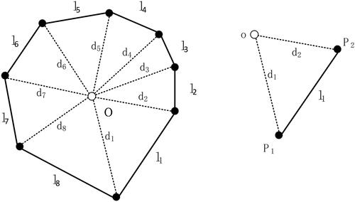
Intuitively, after having the two attributes of a side, it seems that the shape of a building can be restored by inputting these attributes of sides into the neural network in turn. However, for the algorithm, it lacks the relative position information between sides. In order to express the relative position relationship between the sides connected end to end, we use the shape centre $o$ of the contour polygon of the building by imitating the geometric auxiliary line, as shown in Figure 8 and add the link $k_i$ from the midpoint of each side to the centre $o.$ In this way, we use the length $k_i$ and the turning angle $\beta$ of the link to express the structure information of building shape.

Figure 8. Structure information of building shape polygon.

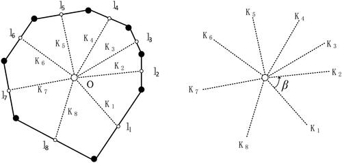
Figure 9. Local information of buildings shape polygon.

3.4.3. Local information of building shape

Theoretically, it can be redrawing the building shape polygon by acquiring detail information and structure information of its shape. However, the description from low-level detail to high-level framework lacks the transition of local shape information, which will be detrimental to partial shape rerecognition, such as partial occlusion. In order to enhance the robustness of the algorithm, we add a step to extract local information of shape. As shown in Figure 9, We define the local area of building polygon shape as a triangle area surrounded by the centre $o$ and two nodes of side $l_i,$ and the local information of the shape is described by extracting the features of $\Delta o{p}_i{p}_{i+1}.$ Here, we select the length of the two sides $d_1$ and $d_2$ of $\Delta o{p}_i{p}_{i+1},$ and the area $s_i$ of the triangle as the local attribute information of the corresponding vertex.

3.4.4. Normalization of vertex attributes

So far, there are 7 attributes of the vertex extracted, which are the length $l$ and the turning angle $\alpha$ of side, the length $k$ and the turning angle $\beta$ of the link, the triangle area $s_i$ and its two sides’ length $d_1,$ $d_2.$ In order to ensure the shape invariance of translation, rotation and scaling and improve the training speed, these attributes are normalized.

Let the perimeter of the shape polygon of the building be $C=\sum l_i,$ then the length of sides in shape polygon are normalized as follows: (19) $$\begin{array}{c}\overline{l}=\frac{l}{C}=\frac{l}{\sum l_i} \end{array}$$(19)

Because the shape of the building is a closed polygon, the turning angle of any side is 360 degrees after a circle along the polygon. Therefore, the turning angle $\alpha$ of the side is normalized to the angle divided by 360. If the counterclockwise orientation is positive, the clockwise orientation is negative. (20) $$\begin{array}{c}\overline{\mathrm{\alpha }}=\frac{\alpha }{360} \end{array}$$(20)

Let $D$ be the sum of the lengths of all the links, and the length of $k_i$ is normalized in the following way: (21) $$\begin{array}{c}\overline{k}=\frac{k}{D}=\frac{k}{\sum k_i}\end{array}$$(21)

The turning angle $\beta$ of the links is normalized in the same way as the turning angle of the sides. (22) $$\begin{array}{c}\overline{\beta }=\frac{\beta }{360}\end{array}$$(22)

Let the sum of the edge lengths between the centre $o$ and the nodes of shape polygon be $Q,$ and then the edge length can be normalized as follows. (23) $$\begin{array}{c}\overline{d_i}=\frac{d_i}{Q}=\frac{d_i}{\sum d_j} \end{array}$$(23)

Let the area of shape polygon be $S,$ and the area of $\Delta o{p}_i{p}_{i+1}$ is normalized as follows. (24) $$\begin{array}{c}{\overline{s}}_i=\frac{s_i}{S}=\frac{s_i}{\sum s_j}\end{array}$$(24)

The normalized attributes of the graph vertices can be expressed as: $X^{(0)}=(\overline{l},\mathrm{ }\overline{\mathrm{ }\mathrm{\alpha }}, \overline{k}, \overline{\beta }, \overline{d_1}, \overline{d_2}, {\overline{s}}_i),$ and they will be the initial inputs of the DGFN model.

4. Experiment and analysis

4.1. Experimental content

In this section, we will design some experiments to verify our understandings of building shape recognition mechanism. To increase the availability of the model, we will also try different hyper parameters to evaluate the shape classification and shape embedding ability of the DGFN model.

4.1.1. Shape classification ability test

4.1.1.1. Graph filter size (k) test

As a multi-layer graph filter model, the graph filter size is a basic parameter. It not only determines the depth of adjacency vertices involved in the filter calculation in each hidden layer, but also affects the propagation speed of vertex attributes in the computation graph. It is an important factor affecting the amount of calculation of each filter. We will try different k values to select the most suitable graph filter size for shape recognition.

4.1.1.2. The dimension of shape embedding and the number of hidden layers test

In the shape classification model, there are two settings related to the dimension. One is the attribute dimension of the vertices in hidden layers; the other is the dimension of graph vector which is aggregated by the vectors of the vertices of the graph. In this experiment, we set them to the same number. Generally speaking, the higher the dimension is, the smaller the information loss will be and the more accurate the classification will be. However, too large dimension will affect the training speed, and in some cases, the model will be too complex and may cause overfitting. So we will test and choose the suitable embedding dimension.

The number of hidden layers refers to the number of graph filter layers used for vertex attributes filtering. Different from convolution neural network, too much attributes aggregation will lead to the information dispersion in the graph convolutional neural network. Some papers suggest that five to seven layers are appropriate (Jian et al. 2017). However, we adopt the idea of multi-layer graph filtering, and we will test whether the superposition of multiple filters will cause information dispersion.

4.1.1.3. The richness of vertex attributes test

Vertex attributes are the kernel information sources of building shape recognition. Therefore, the number of vertex attributes can briefly reflect the richness of shape information. Even though the shape information represented by vertex attributes is not all orthogonal, we also have intuition that the more attributes, the better. We will test the classification accuracy of the DGFN model with different number of attributes.

4.1.1.4. The building shape rotation invariance test

We use relative attribute turning angle instead of absolute attribute azimuth angle to express the orientation of sides in building shape polygon, which can theoretically ensure the rotation invariance of shape recognition. We will construct randomly rotating data to test rotation invariance ability of DGFN model.

4.1.1.5. Compared with similar algorithms

In order to verify the superiority of the classification ability of DGFN model, we select GCN (Kipf and Welling 2016) for comparative experiments, and the two models adopt the same parameters.

4.1.2. Shape embedding ability test

The ability of shape embedding can be understood as the ability of shape expression. To verify the correctness of our idea of embedding pattern, we will compare the shape embedding experimental results with that of DCAE model.

4.2. Experimental datasets

Our experiments in this paper are based on the data set provided by the work of Yan et al. (2021). There are 5010 groups of buildings, which are collected from the open street map (OSM) website. The ones of 5000 ∼ 5009 are 10 standard shapes, and the groups of 0 ∼ 4999 are divided into 10 categories according to 10 standard shapes. Each category has 500 groups data. The 10 standard shapes are shown in Table 1.

Table 1. 10 standard shapes of experimental data.

Standard types	Z- type	H- type	I- type	T- type	L- type	F- type	E- type	O- type	U- type	Y- type
Example shape

In the application of graph convolution network, the number of vertices in each graph is required to be consistent. But the number of vertices of the computation graph is different due to the variety of the number of sides in shape polygon. Therefore, it is necessary to unify the number of the graph vertices. To solve this problem, some algorithms use the max number of vertices of the polygon as the benchmark and encrypt the nodes of the shape polygons of other buildings. There are also algorithms that increase the number of unconnected vertices to ensure a fixed number of vertices (Nina et al. 2019). However, these methods will increase the unnecessary burden of training. We choose the solution provided by DGL, which uses multiple graphs to form a batch. A batch makes up a large graph, of which the number of vertices is fixed. And there is no connection between the graphs in the batch, which can naturally achieve the consistency of vertex number of each computation graph.

4.3. Shape classification experiments

4.3.1. Metrics of shape classification

The metrics of multi-classification task are derived from metrics of binary classification task, which is generally based on confusion matrix. The metrics mainly include accuracy, precision, recall and F₁. We also use these four metrics to measure the classification ability of the DGFN model. Different from binary classification, each metric in multi-classification model is divided into macro average and micro average. In this paper, the macro average is adopted. Supposing there are n classes, if $F_{1i}$ denotes the $F_1$ of class $i,$ then $\mathit{Macro}-F_1$ of all test sets is (25) $$\begin{array}{c}{\mathit{Macro}-F}_1=\frac{1}{n}\sum _{i=1}^n{F}_{1i}\mathrm{ } \end{array}$$(25)

Similarly, the other metrics are defined as follows. (26) $$\begin{array}{c}M\mathit{acro}-\mathit{accuracy}=\frac{1}{n}\sum _{i=1}^n{\mathit{accuracy}}_i \end{array}$$(26) (27) $$\begin{array}{c}M\mathit{acro}-\mathit{precision}=\frac{1}{n}\sum _{i=1}^n{\mathit{precision}}_i\end{array}$$(27) (28) $$\begin{array}{c}M\mathit{acro}-\mathit{recall}=\frac{1}{n}\sum _{i=1}^n{\mathit{recall}}_i\mathrm{ } \end{array}$$(28)

4.3.2. Graph filter size (k) test

To test the influence of the graph filter size k, we have set the k = 1, 2, 3 and observed the performance when the model has three-layer, four-layer, five-layer graph filters. And in the experiments, the dimension of the embedding vectors is set to 256. The network training process is shown in Figure 10.

Figure 10. Training loss curve and validation accuracy curve with different k values.

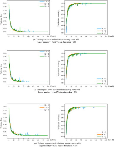
From the loss curve, it can be seen that with the three-layer graph filters, the larger the k value is, the faster the loss value decreases. This is also can be seen from the change of accuracy curve. This indicates that a larger k value will accelerate the training process. With the increase of the number of hidden layers, the difference of training speed and training accuracy gradually disappears.

Table 2 shows the results of experiments with different k values and different graph embedding dimensions. The black bold numbers in the table represent the best validation accuracy for that parameter setting. From the results, it can be seen that k = 2 is the best. It shows that the second-order filtering can achieve better effect for the recognition of building shape. Therefore, we set k to 2 in the following experiments.

Table 2. Validation accuracy of different k value.

Hidden layer number	Vector dimension	k = 1			k = 2			k = 3
		Macro- precision	Macro- recall	Macro- F1	Macro- precision	Macro- recall	Macro- F1	Macro- precision	Macro- recall	Macro- F1
1	128	0.85923	0.85744	0.8583	0.87956	0.8772	0.8784	0.86468	0.86139	0.863
	256	0.89616	0.88813	0.8921	0.88207	0.8792	0.8806	0.91189	0.9109	0.9114
2	128	0.95461	0.95347	0.954	0.96256	0.96237	0.9625	0.95236	0.95248	0.9524
	256	0.95396	0.95347	0.9537	0.96768	0.96634	0.967	0.95489	0.95347	0.9542
3	128	0.98025	0.9802	0.9802	0.98262	0.98217	0.9824	0.96753	0.96733	0.9674
	256	0.98342	0.98317	0.9833	0.98235	0.98217	0.9823	0.98171	0.98119	0.9814
4	128	0.98548	0.98515	0.9853	0.97967	0.9792	0.9794	0.97441	0.97426	0.9743
	256	0.98624	0.98614	0.9862	0.9842	0.98415	0.9842	0.97249	0.97228	0.9724
5	128	0.97289	0.97228	0.9726	0.97971	0.97920	0.9795	0.97926	0.97921	0.9792
	256	0.98718	0.98713	0.9872	0.98447	0.98415	0.9843	0.97965	0.97921	0.9794

4.3.3. The dimension of shape embedding and the number of hidden layers test

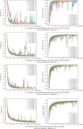
Figure 11 shows the training process when the embedding dimensions are 32, 64, 128 and 256, and the number of hidden layers is 1–9. From the decline process of the loss curve, we can see that with the increase of the embedding dimension, the training speed of the model is accelerated. From the trend of the validation accuracy curve, the training accuracy is gradually improved with the increase of the embedding dimension. When the embedding dimensions are 32 and 64, the model’s loss curve shows significant fluctuations, especially when the number of layers is one and two. Lower embedding dimensions may cause the model to struggle in capturing enough information for accurate data representation. Additionally, it limits the expression of input features, posing a challenge for precise differentiation between data categories and, consequently, leading to unstable model performance. This trend is evident in the accuracy curve. As both the embedding dimension and the number of convolutional layers increase, the model’s fluctuations become less pronounced, leading to a gradual improvement in training accuracy. In general, the model performs admirably with an embedding dimension of 256.

Figure 11. Training process with different embedding dimension and layer numbers.

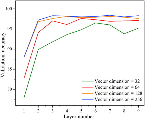
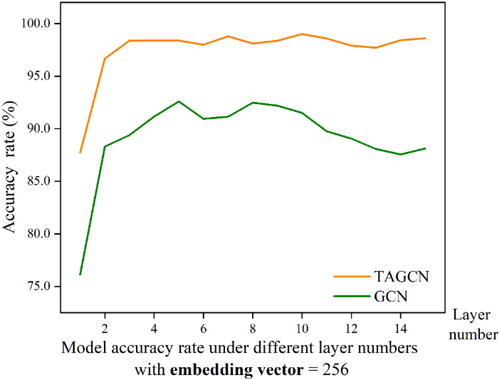
Figure 12 shows the comparison of the validation accuracy when the convolution layer is 1–9 and the embedding dimensions are 32, 64, 128 and 256 respectively. From the figure we can see that the model with 32-embedding-dimension achieves the highest validation accuracy when the hidden layer is 6, which is significantly lower than that of other dimensions, indicating that the loss of shape information is relatively serious. The validation accuracy with 64-embedding-dimension is slightly lower than that of the other two dimensions, and the training efficiency is also slightly lower. There is little difference between the validation accuracy with 128 and 256 embedding-dimension. The training accuracy of 256-embedding-dimension is slightly higher, but the training efficiency of 128-embedding-dimension is higher.

Figure 12. Validation accuracy of different embedding dimensions.

4.3.4. Buildings random rotation invariance test

This experiment is to rotate the shape polygon randomly within the scope of ($-180°,180°)$ with the centre of the shape polygon as the origin. The maps used in experiment are shown in Figure 13. Figure 14 shows the training and validation process before and after random rotation. The blue curve shows the result using the data before rotation, and the yellow curve is that using the data after random rotation. And the number of layers has been set to 4, 8 and 12. From the results, it can be seen that both the train loss curve and the validation accuracy curve are basically coincident, which shows that the data distribution and training process are not affected by the shape random rotation.

Figure 13. Example of building random rotation test.

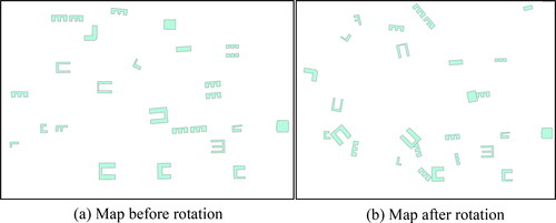
Figure 14. Training process before and after shape random rotation.

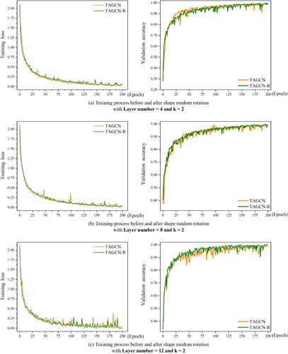
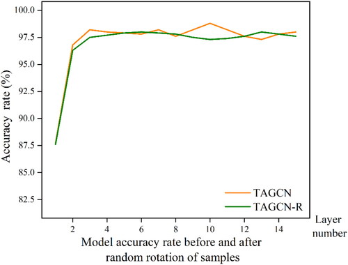
Figure 15 shows the comparison of classification accuracy of the model before and after random rotation. The blue curve is the results before rotation and the yellow curve is that after rotation. The two curves have little difference, which is consistent with the random distribution of data. This indicates that the classification ability of DGFN model is random rotation invariance. Thus, the DGFN model efficiently utilizes architectural shape data from various perspectives, partially reducing computational complexity and improving the model’s generalization capabilities.

Figure 15. Comparison of classification accuracy before and after random rotation.

4.3.5. The richness of vertex attributes test

To test the influence of different number of vertex attributes, we have adopted 2 attributes (side length $\overline{l}$ and turning angle $\overline{\mathrm{\alpha }}$), 4 attributes (the above two attributes plus attributes of polygon structure, which is $\overline{k}$ and $\overline{\beta }$), 7 attributes (the above four attributes plus three attributes of the local triangle, which is $\overline{d_1}, \overline{d_2}, {\overline{s}}_i$) in different experiments to observe the performance of the DGFN model. The comparisons of training process of two-layer, four-layer and six-layer model are shown in Figure 16.

Figure 16. Training loss curve and validation accuracy curve with different attributes number.

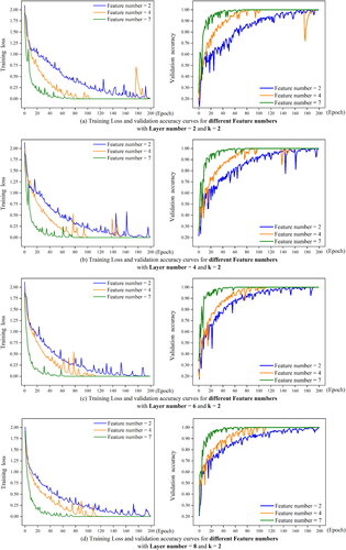
From the training loss and validation accuracy figures, it can be seen that no matter how the number of hidden layers increases, the decline rate of loss curve and the rising rate of validation accuracy curve of two-attribute model are the lowest, and the highest validation accuracy of two-attribute model is about 90% at six hidden layers. When the number of hidden layers is 2, the validation accuracy of four-attribute model and seven-attribute model is similar, and the training efficiency of seven-attribute model is slightly higher. With the increase of the number of hidden layers, the accuracy of seven-attribute model is improved significantly, which indicates that more sufficient shape information is helpful for shape classification. The change of training speed also indicates that rich attributes are helpful to shape recognition.

4.3.6. Comparisons with GCN

To compare with the GCNs (Indolia et al. 2018), we have set the dimension of embedding vector to 256. Figure 17 shows the changes of the loss and the accuracy during the training process when both models adopt three, four, five, six layers, and Figure 18 shows the comparison of classification accuracy of the two models.

Figure 17. Training process comparison of DGFN and GCN model.

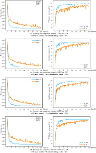
Figure 18. Comparison of classification accuracy between DGFN and GCN model.

According to the classification accuracy in Table 3, with the same number of hidden layers, the loss of DGFN model declines faster than that of GCN, and the validation accuracy is higher than that of GCN. This indicates that it is easier to train the DGFN model. The optimal training accuracy of GCN is 0.9258 when the number of hidden layers is 5, and the training accuracy decreases with the increase of hidden layer number. After the classification accuracy of DGFN model reaches 98% with three hidden layers, it maintains relatively high classification accuracy and does not reduce the classification ability with the increase of hidden layer number. This indicates that the model has a strong data adaptability and application potential. All these show that DGFN is better than GCN for this task.

Table 3. Classification accuracy comparisons of DGFN and GCN model.

Layer	TAGCN	GCN	Layer	TAGCN	GCN	Layer	TAGCN	GCN
1	0.8773	0.7613	6	0.9798	0.9094	11	0.9859	0.8975
2	0.9668	0.883	7	0.9879	0.9114	12	0.9790	0.8905
3	0.9836	0.8938	8	0.9810	0.9247	13	0.9770	0.8807
4	0.9838	0.9116	9	0.9836	0.9218	14	0.9841	0.8754
5	0.9838	0.9258	10	0.9900	0.915	15	0.986	0.8812

4.4. Shape embedding experiments

4.4.1. Metrics of shape embedding ability

We use four metrics to measure the shape embedding ability of DGFN model, which are Nearest neighbour, First Tier, Second Tier and Normalized Discounted Cumulative Gain.

• Nearest neighbour (NN): NN refers to the number of objects that belong to the same shape type as their closest neighbour to the total number of training data. This metric represents the shape resolution of the model at single object level.

• First tier (FT) and second tier (ST): for a certain type, if sorted by vector distance, FT and ST refer to the percentages of shapes that belong to the same type as it does in its top (t − 1) and 2(t − 1) neighbours. Different from NN, FT and ST consider the population distribution status and position of the same kind of objects relative to the typical vector.

• Normalized Discounted Cumulative Gain (NDCG): NDCG is the location distribution relationship of similar objects relative to the typical vector of the category. Generally, the distribution of queried objects is expressed by cumulative revenue (CG). DCG introduces a penalty function based on logarithm to reduce the correlation score of each location. In order to facilitate the comparison of multi types and cross type query, the value of DCG is normalized by idealized order, which is NDCG.

The values of all the above metrics are in the range of (0,1), and the larger the value is, the better the result is.

4.4.2. Coding experiments in embedding pattern

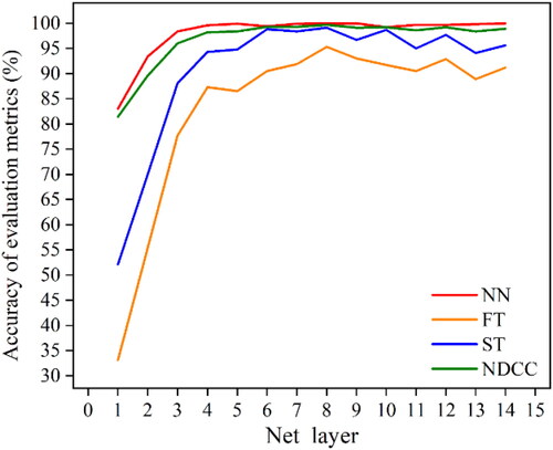
Table 4 shows the experimental results of shape coding ability in embedding pattern of DGFN model when there are different numbers of hidden layers. From these results, it can be seen that the model has good coding ability when there are more than four hidden layers. The experimental results reach the peak when the number of hidden layers is 8. Especially the FT metrics reaches 0.953, which means most of them are in the top (t − 1) position, and the number of objects in the interval (t − 1, 2t − 1) is only 0.038. The NDCG’s peak value also reaches 0.997, which indicates that the ranking of similar objects is close to the ideal value.

Table 4. Experimental results of shape coding in embedding pattern of DGFN.

Layer	NN	FT	ST	NDCG	Layer	NN	FT	ST	NDCG
1	0.83	0.331	0.521	0.814	8	1.0	0.953	0.991	0.997
2	0.934	0.554	0.7	0.896	9	1.0	0.93	0.967	0.991
3	0.984	0.777	0.881	0.96	10	0.992	0.917	0.987	0.992
4	0.996	0.873	0.943	0.982	11	0.997	0.905	0.95	0.986
5	0.999	0.865	0.948	0.984	12	0.997	0.929	0.977	0.992
6	0.994	0.905	0.988	0.993	13	0.998	0.889	0.941	0.984
7	0.999	0.919	0.984	0.993	14	1.0	0.912	0.956	0.989

It can be seen from Figure 19 that in the process of increasing the hidden layer number from 1 to 4, every metric value has been significantly improved, which shows that shape embedding needs a certain number of hidden layers. When the number of layers exceeds 4, the value of each metrics fluctuates little, which indicates that the model has stable shape expression ability after neural network convergence.

Figure 19. Shape embedding metrics curve with different hidden layers.

4.4.3. Comparison with GCAE models

Figure 20 shows the results of embedding experiments of DGFN model with different embedding dimensions when compared with GCAE model. It can be seen that each metric with 32-emdeding-dimension is low, which indicates that too low embedding dimension will lead to information loss and impair the shape expression ability of the model. With the increase of the embedding dimensions, each metric value has a corresponding improvement. From the experiment results, the metrics value of DGFN model is not only better than the original GCAE model, but also better than the GCAE (R) model after manually adjusting the orientation of buildings shape, indicating that DGFN model has excellent shape expression ability, and this ability is not affected by the orientation, size and location of building.

Figure 20. Accuracy rates of shape embedding metrics with different models.

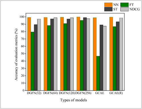
Figure 21. Dimension reduction visualization of embedded graph vectors.

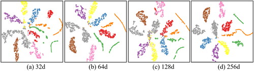
4.4.4. Visualization of vectors with different embedding dimensions

Figure 21 shows the dimensionality reduction visualization of graph vectors when the embedding dimensions are 32, 64, 128 and 256. It can be seen that the graph vectors of each dimension have achieved different degrees of clustering, and the distance be-tween clusters is obvious. It is worth noting that with the increase of embedding dimension, the classification between categories becomes more and more clear, and there is a secondary clustering within categories, which indicates that there may be a problem of disunity in the level of manual classification.

5. Conclusion

Inspired by the graph signal processing theory, we regard shape recognition as a multi-level nonlinear graph signal filtering process and propose a novel DGFN model for the shape recognition of the buildings in maps. By comparing with the traditional GCN and GCAE models, the proposed DGFN model has advantages in accuracy and robustness. Compared to the existing works on building shape recognition, the highlights of our work are as follows:

1. We use the sides of shape polygon as the basic units to construct the computation graph of building. This lays a good foundation for subsequent attribute extraction and vertex signal filtering.

2. A method of extracting the vertex attributes of building shape is proposed, which takes into account the shape details, shape structure and shape local information. This method only needs a small number of attributes to describe the characteristics of building shape.

3. We use relative features instead of absolute features to express shape information. This measure helps to realize the shape recognition of building with scaling, rotation, displacement invariance and improves the usability and robustness of the algorithm.

4. We build a deep graph filter neural network model which deeply excavates the advantages of TAGCN graph filter in graph classification and realizes the end-to-end building shape embedding and classification.

Following experimental testing and analysis, we found that the optimal Graph filter size (k) value for the DGFN model is 2. Moreover, setting the embedding vector dimension to 256 results in significantly improved accuracy in shape classification for the model. In these scenarios, with 8 hidden layers, the model’s shape embedding metrics, such as NN, FT, ST and NDCG, all attain their peak values, signifying optimal shape embedding. Compared to similar models such as GCN for graph classification and GCAE for graph embedding, our DGFN model excels in both classification and embedding capabilities.

In our study of spatial building shape classification, we have placed relatively less emphasis on spatial cognition and instead focused more on designing a model that encompasses both shape classification and shape embedding. Nevertheless, this aspect demands additional research and refinement in future investigations. Additionally, given the diverse nature of building shapes, there are still numerous buildings that do not fit into predefined categories. The challenge of identifying the shapes of these irregular buildings remains unresolved. Classifying and recognizing building shapes in an adaptive manner based on the area’s shape characteristics is also an intriguing and demanding challenge.

Acknowledgements

Special thanks to the editor and anonymous reviewers for their insightful comments and constructive suggestions that substantially improved the quality of the paper.

Disclosure statement

No potential conflict of interest was reported by the author(s).

Additional information

Funding

This work was supported by the National Natural Science Foundation of China (Grant No. 42271463). Higher Education Teaching Reform Research Project of Henan Province, Grant/Award Number: 2021SJGLX299; Natural Science Foundation for Distinguished Young Scholars of Henan Province, Grant/Award Number: 212300410014. Key Scientific Research Projects of Universities in Henan Province, Grant/Award Number: 22B420001.

References

- An X, Sun Q, Xiao Q, Yan W. 2011. A shape multilevel description method and application in measuring geometry similarity of multi-scale spatial data. Acta Geod Cartogr Sin. 40(4):495–501+508. doi: 10.1007/s11442-011-0836-7
- Bruna J, Zaremba W, Szlam A, Lecun Y. 2013. Spectral networks and locally connected networks on graphs. Computer Science. doi: 10.48550/arXiv.1312.6203
- Guo H, Du B, Zhang L, Su X. 2022. A coarse-to-fine boundary refinement network for building footprint extraction from remote sensing imagery. ISPRS J Photogramm Remote Sens. 183:240–252. doi: 10.1016/j.isprsjprs.2021.11.005.
- Haiwei H, Haizhong Q, Limin X, Peixiang D. 2018. Interchange recognition method based on CNN. Acta Geod Cartogr Sin.47: 385–395. doi: 10.11947/j.AGCS.2018.20170265
- Henn A, Römer C, Gröger G, Plümer L. 2012. Automatic classification of building types in 3D city models. Geoinformatica. 16(2):281–306. doi: 10.1007/s10707-011-0131-x.
- Indolia S, Goswami AK, Mishra SP, Asopa P. 2018. Conceptual understanding of convolutional neural network- A deep learning approach. Proc Comput Sci. 132:679–688. doi: 10.1016/j.procs.2018.05.069.
- Jian D, Zhang S, Wu G, Moura J, Kar S. 2017. Topology adaptive graph convolutional networks. doi: 10.48550/arXiv.1710.10370
- Kim Y. 2014. Convolutional neural networks for sentence classification. Proceedings of the 2014 Conference on Empirical Methods in Natural Language Processing (EMNLP), Doha, Qatar. Association for Computational Linguistics. p. 1746–1751. doi: 10.3115/v1/D14-1181
- Kipf TN, Welling M. 2016. Variational graph auto-encoders. ArXiv, abs/1611.07308. doi: 10.48550/arXiv.1611.07308
- Krizhevsky A, Sutskever I, Hinton GE. 2017. ImageNet classification with deep convolutional neural networks. Commun ACM. 60(6):84–90. doi: 10.1145/3065386.
- Li C, Zhang H, Wu P, Yin Y, Liu S. 2020. A complex junction recognition method based on GoogLeNet model. Trans GIS. 24(6):1756–1778. doi: 10.1111/tgis.12681.
- Liu Y, Chen D, Ma A, Zhong Y, Fang F, Xu K. 2021. Multiscale U-shaped CNN building instance extraction framework with edge constraint for high-spatial-resolution remote sensing imagery. IEEE Trans Geosci Remote Sensing. 59(7):6106–6120. doi: 10.1109/TGRS.2020.3022410.
- Liu Y, Gross L, Li Z, Li X, Fan X, Qi W. 2019. Automatic Building extraction on high-resolution remote sensing imagery using deep convolutional encoder-decoder with spatial pyramid pooling. IEEE Access. 7:128774–128786. doi: 10.1109/ACCESS.2019.2940527.
- Mark DM, Freksa C, Hirtle SC, Lloyd R, Tversky B. 1999. Cognitive models of geographical space. Int J Geograph Inf Sci. 13(8):747–774. doi: 10.1080/136588199241003.
- Nina M, Andong W, Xiaodong Z. 2019. A graph convolutional neural network method for pattern recognition of linear building alignment. J Geomatics Sci Technol. 36(6):627–631.
- Ortega A, Frossard P, Kovacevic J, Moura JMF, Vandergheynst P. 2018. Graph signal processing: overview, challenges, and applications. Proc IEEE. 106(5):808–828. doi: 10.1109/JPROC.2018.2820126.
- Sandryhaila A, Moura JMF. 2013. Discrete signal processing on graphs. IEEE Trans Signal Process. 61(7):1644–1656. doi: 10.1109/TSP.2013.2238935.
- Shelhamer E, Long J, Darrell T. 2017. Fully convolutional networks for semantic segmentation. IEEE Trans Pattern Anal Mach Intell. 39(4):640–651. doi: 10.1109/TPAMI.2016.2572683.
- Shi Y, Li Q, Zhu XX. 2020. Building segmentation through a gated graph convolutional neural network with deep structured feature embedding. ISPRS J Photogramm Remote Sens. 159:184–197. doi: 10.1016/j.isprsjprs.2019.11.004.
- Steiniger S, Lange T, Burghardt D, Weibel R. 2008. An approach for the classification of urban building structures based on discriminant analysis techniques. Trans GIS. 12(1):31–59. doi: 10.1111/j.1467-9671.2008.01085.x.
- Szegedy C, Wei L, Yangqing J, Sermanet P, Reed S, Anguelov D, Erhan D, Vanhoucke V, Rabinovich A. 2015. Going deeper with convolutions. In: 2015 IEEE Conference on Computer Vision and Pattern Recognition (CVPR), Boston, Ma, USA, p. 1–9. doi: 10.1109/CVPR.2015.7298594.
- Tang W, Hao Y, Zhao Y, Li N. 2008. Research on areal feature matching algorithm based on spatial similarity. Chinese Control and Decision Conference, Yantai, Shandong, p. 3326–3330. doi: 10.1109/CCDC.2008.4597945.
- Tianyuan X, Pengcheng L, Tinghua A, Jingzhong L. 2020. A fractal description and multi-scale expression method of Fourier information metrics. Geomatics and Information Science of Wuhan University; 45(1): 119–125. doi: 10.13203/j.whugis20180336
- Velikovi P, Cucurull G, Casanova A, Romero A, Liò P, Bengio Y. 2017. Graph attention networks.arXiv preprint arXiv:1710.10903. doi: 10.48550/arXiv.1710.10903
- Wang H, Wu F, Zhang L, Deng H. 2005. The application of mathematical morphology and pattern recognition to building polygon simplification. Acta Geodaetica et Cartographic Sinica. 34:269–276.
- Wang S, Hou X, Zhao X. 2020. Automatic building extraction from high-resolution aerial imagery via fully convolutional encoder-decoder network with non-local block. IEEE Access. 8:7313–7322. doi: 10.1109/ACCESS.2020.2964043
- Wei S, Zhang T, Ji S, Luo M, Gong J. 2023. BuildMapper: a fully learnable framework for vectorized building contour extraction. ISPRS J Photogramm Remote Sens. 197:87–104. doi: 10.1016/j.isprsjprs.2023.01.015.
- Xiaohua T, Susu D, Wenzhong SHI. 2007. A probabilistic theory-based matching method. Acta Geod Cartogr Sin. 36:210–217.
- Xu Y, Chen Z, Xie Z, Wu L. 2017. Quality assessment of building footprint data using a deep autoencoder network. Int J Geograph Inf Sci. 31(10):1929–1951. doi: 10.1080/13658816.2017.1341632.
- Yan X, Ai T, Yang M. 2016. A simplification of residential feature by the shape cognition and template matching method. Acta Geod Cartogr Sin. 45:874–882.
- Yan X, Ai T, Yang M, Tong X. 2021. Graph convolutional autoencoder model for the shape coding and cognition of buildings in maps. Int J Geograph Inf Sci. 35(3):490–512. doi: 10.1080/13658816.2020.1768260.
- Yang M, Ai T, Yan X, Chen Y, Zhang X. 2018. A map-algebra-based method for automatic change detection and spatial data updating across multiple scales. Trans GIS. 22(2):435–454. doi: 10.1111/tgis.12320.
- Zhao K, Kang J, Jung J, Sohn G. 2018. Building extraction from satellite images using mask R-CNN with building boundary regularization. IEEE/CVF Conference on Computer Vision and Pattern Recognition Workshops (CVPRW), Salt Lake City, UT, USA, 2018, p. 242–2424. doi: 10.1109/CVPRW.2018.00045.
- Zhou X, Chen Z, Zhang X, Ai T. 2018. Change detection for building footprints with different levels of detail using combined shape and pattern analysis. IJGI. 7(10):406. doi: 10.3390/ijgi7100406.
- Zonghan W, Shirui P, Fengwen C, Guodong L, Chengqi Z, Philip S Y. 2020. A comprehensive survey on graph neural networks. IEEE Transactions on neural networks and learning systems 1:32.