Spatial prediction of groundwater potential by various novel boosting-based ensemble learning models in mountainous areas

Abstract

This study makes a significant contribution to the field of groundwater potential mapping (GWPM) by exploring the application of ensemble learning models (ELMs), specifically boosting ensemble models (BEMs), which have not been fully utilized in GWPM. By employing six ELMs (random forest, AdaBoost, XGBoost, CatBoost, GBDT and LightGBM), along with Tree-structured Parzen Estimator in Luoning County, China, this study identifies key indicators (topographic position index, distance to rivers and topographic wetness index) and demonstrates the superior model performance of XGBoost compared to other ELMs. Additionally, correlation analysis confirms the accuracy of XGBoost in predicting relationships between important indicators and groundwater potentials. Finally, the findings provide valuable insights for sustainable groundwater management strategies in Luoning County and emphasize the need for further exploration of ELMs, development of comprehensive performance evaluation and indicator systems, reduction of the inconsistencies between indicators and predication results and practical research to support future sustainable groundwater management.

Keywords:

• Groundwater potential mapping
• ensemble learning models
• boosting algorithm
• sustainable groundwater management

1. Introduction

Groundwater is an essential natural resource that plays a vital role in supporting economic, social and environmental development worldwide (Xiong et al. 2022; Guo et al. 2023b). Compared to other water resources, groundwater has significant advantages of high quality, wide distribution, constant chemical composition, reliability during drought and low development cost (Chowdhury et al. 2009; Jha et al. 2009; Chen et al. 2019). However, the global demand for groundwater has led to widespread and uncontrolled exploitation in various regions (Green et al. 2011), resulting in numerous environmental issues. These issues include land subsidence (Li et al. 2021), groundwater salinization (Pulido-Bosch et al. 2018), groundwater level depletion and fluctuation (Taheri et al. 2016; Monir et al. 2023), hydraulic connections decrease (Kustu et al. 2010), groundwater contamination (Salcedo-Sánchez et al. 2016), vegetation degradation (Zhao et al. 2005), ecosystem deterioration (Zhang et al. 2014) and water resource imbalance (Liu et al. 2018). Considering the widespread droughts caused by climate change, the adverse effects of excessive exploitation are likely to worsen in the future (Mustafa et al. 2017; Hamed et al. 2018). Consequently, sustainable groundwater exploitation and management have become significant focus for scholars worldwide (Gaye and Tindimugaya 2019; Jia et al. 2019; Jesiya and Gopinath 2020; Priya et al. 2022).

Groundwater potential mapping (GWPM) provides valuable information regarding the quantity of exploitable groundwater from the aquifer without negatively impacting groundwater yield and environmental conditions (Thanh et al. 2022). During drought periods, water managers and authorities rely on GWPM to identify new springs and areas with high groundwater potential (GWP) to augment water resources (Naghibi and Moradi Dashtpagerdi 2017). Moreover, GWPM plays a crucial role in supporting various sustainable water management activities, including groundwater exploitation, water resource allocation, water policy implementation and groundwater conservation (Ozdemir 2011a; Moghaddam et al. 2015; Naghibi and Pourghasemi 2015; Sarkar et al. 2022a). Traditional methods for GWPM such as sample drilling, ground surveys and hydrological lab tests are challenging, costly, inefficient and time-consuming. The integration of geographic information system (GIS) and remote sensing (RS) has significantly simplified the GWPM process and improve the prediction accuracy (Nampak et al. 2014; Amade et al. 2018; Rizeei et al. 2019). The methods for GWPM normally include knowledge-based methods (e.g. analytical hierarchy process), traditional statistical methods (e.g. frequency ratio, influencing factor and weight of evidence) and machine learning (ML) methods, while ML models have gained more popularity in GWPM due to their superiority in model performance over other two groups of methods (Pham et al. 2019; Thanh et al. 2022). In these ML models, two approaches can be employed to assess GWPs: springs and wells. For spring datasets, an equal number of non-spring dataset are created for training and testing purposes (Chen et al. 2018; Rahmati et al. 2018; Kordestani et al. 2019). For well datasets, the wells can be classified as productive wells and unproductive wells (Machiwal et al. 2015; Shabani et al. 2022).

Numerous popular ML models have been extensively applied in GWPM, including logistic regression (Ozdemir 2011b), artificial neural network (Lee et al. 2018), discriminant analysis (Naghibi and Moradi Dashtpagerdi 2017), support vector machine (Prasad et al. 2020), k-nearest neighbor (Al-Abadi et al. 2021) and decision tree (Chen et al. 2020). However, these models still have some limitations. For example, they often rely on assumptions linking GWPs and indicators (Umar et al. 2014; Termeh et al. 2019), lack comprehensive explanations of the internal modeling process (Lee et al. 2018), high sensitivity to extreme values and scare data (Gambella et al. 2021) and overfitting issue (Thanh et al. 2022). Many scholars have pointed out that ensemble models, including bagging, boosting and stacking algorithms, have the potential to address some of the above limitations and achieve better model performances in GWPM (Moghaddam et al. 2020; Gomez-Escalonilla et al. 2022; Mallick et al. 2022; Rasool et al. 2022; Sarkar et al. 2022b; Talukdar et al. 2022). However, the exploration of ensemble learning models (ELMs), especially boosting ensemble models (BEMs), is still in its early stages for GWPM (Chen et al. 2020). In fact, many advantages are included in BEMs, such as their capacity to capture nonlinear relationships, identify important indicators and overcome overfitting issues. Consequently, there is a critical need to investigate the application and performance of BEMs in GWPM, as it will unlock their full potential and provide valuable insights for water resource management, decision making and the implementation of sustainable water management practices.

BEMs employ an iterative method to construct a powerful classifier by assembling a series of weak learners. The array of weak learners commonly consists of a combination of classification and regression forms (Zhang and Ma 2012). Table 1 presents a comprehensive overview of the BEMs employed in GWPM, with BEMs highlighted in bold. Several observations can be found from Table 1. Firstly, a majority of the BEMs had higher model performance than other ML models. It fully demonstrates the great potential of BEM in GWPM for model performance improvement. Secondly, many high-performing BEMs, namely AdaBoost, CatBoost, XGBoost, LightGBM and GBDT have not been fully explored in GWPM despite their wide adoption in various sectors such as groundwater vulnerability assessment (Naghibi et al. 2020), flash-flood susceptibility (Abedi et al. 2022), forest fire susceptibility (Sun et al. 2022), landslide susceptibility (Sahin 2022) and wind power forecasting (Ju et al. 2019). These algorithms are considered effective in these studies and show different significant advantages. Specifically, AdaBoost focuses on correcting misclassified instances by adjusting their weights (Freund and Schapire 1997), while CatBoost is optimized for handling categorical features (Prokhorenkova et al. 2018). XGBoost uses a more regularized model formalization to control over-fitting and improve model performance (Chen and Guestrin 2016), and LightGBM is designed for efficiency and scalability, especially with large datasets (Ke et al. 2017). GBDT can serve as a general framework that underpins many of these methods for modeling (Friedman 2001). Thirdly, there exists a scarcity of comprehensive comparative studies that adequately evaluate and benchmark the performance of BEMs in GWPM. The critical need for detailed assessments of these models’ predictive accuracy in GWPM is evident, but such crucial investigations are currently lacking in the literature. Consequently, it is important to further explore the use of these BEMs in GWPM, as they offer significant potential for improving prediction accuracy and achieving sustainable groundwater management.

Table 1. BEMs and top performance models that have been used in GWPM.

Studies	Models	Top performance models
Rasool et al. (2022)	ANN, RF, SVM, KNN, NB, XGBoost	XGBoost, RF
Chen et al. (2020)	RF-J48, AB-J48, Bag-J48, RS-J48, Dag-J48	RF-J48, AB-J48
Naghibi et al. (2020)	RF, PRF, XGB-Linear, XGB-DART, XGB-Tree	PRF, XGB-Linear
Naghibi et al. (2016)	BRT, CART, RF	BRT
Chen et al. (2022)	BT, ANN, DLNN, DLT, DB	DB, BT
Sachdeva and Kumar (2021)	GBDT, RF	GBDT
Park and Kim (2021)	RF, GBM, XGBoost	XGBoost
Kamali Maskooni et al. (2020)	LMT, DB, BRT, RF, KNN	LMT, DB
Mousavi et al. (2017)	BRT, FR	BRT
Naghibi and Pourghasemi (2015)	CART, BRT, RF, EBF, GLM	CART, BRT
Prasad et al. (2020)	RF, BRT, RF-SVM	RF
Wei et al. (2022)	BMA, RF, GBDT	GBDT
Al-Fugara et al. (2020)	RF, BRT, SVM, MDA, MARS	MDA, RF
Yen et al. (2021)	AB, Bag, MB, RTF, LWL	ABLWL, MBLWL
Naghibi et al. (2018)	RF, SVM, BRT, FDA, MARS, QDA, LDA, PDA, KNN, ANN	RF, SVM, BRT
Lee et al. (2019)	BT, FR	BT
Yousefi et al. (2020)	RF-BRT, MARS-SVM, FDA-GLM-MDA	RF-BRT
Kim et al. (2019)	BRT, RF, LR	LR
Naghibi et al. (2017b)	FREM, AB, Bag, GAM, NB	FREM, Bag

Note: Bold texts refer to BEMs and abbreviations have been modified from original authors (ANN: Artificial Neural Network; RF: Random Forest; SVM: Support Vector Machine; KNN: K-Nearest Neighbor; NB: Naïve Bayes; XGBoost: Extreme Gradient Boosting; J48: J48 Decision Trees; AB: AdaBoost; Bag: Bagging; Dag: RS: RandomSubSpace; Dag: Dagging; PRF: Parallel Random Forest; XGB-Linear: Extreme Gradient Boosting with linear booster; XGB-DART: Extreme Gradient Boosting with DART booster; XGB-Tree: Extreme Gradient Boosting with tree booster; BRT: Boosted Regression Tree; CART: Classification and Regression Trees; BT: Boosted Tree; DLNN: Deep Learning Neural Network; DLT: Deep Learning Tree; DB: Deep Boosting; GBDT: Gradient Boosting Decision Tree; GBM: Gradient Boosting Machine; LMT: Boosted Regression Tree; DB: Deep Boosting; GLM: General Linear Model; EBF: Evidential Belief Function; BMA: Bayesian Model Averaging; MDA: Mixture Discriminant Analysis; MARS: Multivariate Adaptive Regression Spline; MB: Multi Boost; RTF: Rotation Forest; LWL: Locally Weighed Learning; FDA: Flexible Discriminant Analysis; QDA: Quadratic Discriminant Analysis; PDA: Penalized Discriminant Analysis; FREM: Frequency Ratio Data Mining; GAM: Generalized Additive Model).

The indicators for assessing GWP can be classified into various aspects, including topographic, geological, hydrological, climatic, land cover and aquifer aspects (Thanh et al. 2022). In mountainous areas, topographic and hydrological indicators likely have a more significant impact on GWP prediction due to the complex landscape and terrain. However, few studies have comprehensively considered these two indicator groups in mountainous areas. Moreover, some indicators such as topographic position index (TPI), terrain ruggedness index (TRI), stream power index (SPI) and slope length (SL) have not been thoroughly investigated and discussed in relation to GWPM. It is also worth noting that many previous studies previous studies have primarily concentrated on a limited set of indicators, typically comprising fewer than fifteen indicators. This limited range of indicators may not be sufficient for achieving accurate model performance.

In light of the aforementioned, this study aims to comprehensively evaluate and compare the predictive performance of five specific BEMs, including AdaBoost, GBDT, CatBoost, XGBoost and LightGBM for GWPM by taking Luoning County, China, as the study area. To ensure a robust analysis, RF is employed as a benchmark for comparative purposes. We employ a comprehensive set of 24 indicators encompassing geology, climate, hydrology, topography, land use and human activity for GWPM. These indicators are carefully selected to provide a comprehensive understanding of the factors that may potentially influence GWP. To optimize the performance of the selected models, Tree-structured Parzen Estimator (TPE), as a global hyperparameter optimization method, is used for parameter optimization and model performance improvement. Through evaluation, the optimal model can be identified and subsequently utilized to propose sustainable groundwater management strategies for the study area. This study is distinguished by the following four novel aspects:

1. The study delves into the utilization and comparison of various BEMs (including AdaBoost, XGBoost, LightGBM, CatBoost and GBDT) within the context of GWPM that have not been previously employed or evaluated in this field.

2. TPE approach is employed to identify the globally optimal parameters for the selected models, which is a rarely utilized calibration method within the field of GWPM.

3. The modelling process incorporates a comprehensive array of indicators, including several uncommon ones such as TRI, TPI, SPI and SL.

4. This study contributes a methodology that outlines the incorporation of GWP maps into the development of sustainable groundwater management strategies.

2. Study area

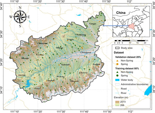
Luoning County, China, covers an area of 2303 km², lying between latitude 34°05′ to 34°40′ North and longitude 111°08′ to 112°49′ East (Figure 1). Characterized by a rich array of bedrock aquifers and diverse terrain, this mountainous region is intersected by the Luohe valley, running from the southwest to the east. The area’s landscape is heavily shaped by its geology and structural conditions, featuring five major landforms (mid-height mountains, low mountains, hilly regions, valleys and alluvial plains) (Sun et al. 2019). Elevations in the study area vary between 266 m and 2073 m above sea level, with slopes ranging from 0° to 61.86°. The areas of high elevation and steep slopes predominantly lie in the southern and western regions, which give birth to the major rivers. In contrast, the central and northeastern areas are relatively flat and low-lying. The study area is characterized by a temperature monsoon climate, with an average annual rainfall of 600 mm to 800 mm and the annual average temperature of 13.7 °C (Liang and Liu 2022). The geological profile of the area features 17 types of rock, with Migmatite, Quartzite and Biotite granite being most common River plains are largely covered by alluvial soil, while brown soil is found in forest areas. The primary land use types are cropland and forest. In the face of growing population and increasing pressure on water resources in Luoning County, it is imperative to evaluate GWP to ensure sustainable management of groundwater in the future.

Figure 1. Study area.

3. Methodology

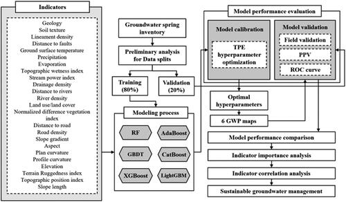
Figure 2 presents the methodological framework employed in this study. This framework encompasses several key steps: data preparation, indicator selection, modeling procedure, model performance assessment and comparison, indicator significance analysis, indicator correlation analysis and sustainable groundwater management strategy formulation. The following section provides a detailed information of this methodology.

Figure 2. Methodology framework.

3.1. Dataset and indicators

The indicators were selected from current literature of GWPM, mainly including Thanh et al. (2022), Moghaddam et al. (2020), Termeh et al. (2019) and Chen et al. (2020). Almost all indicators for GWPM were considered in this study (24 indicators). These indicators can be categorized into geological, climate, hydrological, land use and human activity and topographic aspects. The descriptions of data sources, abbreviations, data types and scales are shown in Table 2.

Table 2. Data sources and indicators.

Indicator types	Indicators	Abbr.	Source	Data type	Scale
Geological indicators	Geology	GEO	RESDC	Shapefile (polygon)	1:250,000
	Lineament density	LD	RESDC	Shapefile (line)	1:250,000
	Distance to faults	DTF	RESDC	Shapefile (line)	1:250,000
	Soil texture	ST	HWSD V1.2	Bil & Mdb	1 km × 1 km
Climate indicators	Ground surface temperature	GST	RESDC	Raster	1 km × 1 km
	Precipitation	PRE	RESDC	Raster	1 km × 1 km
	Evaporation	EVA	RESDC	Raster	1 km × 1 km
Hydrological indicators	Topographic wetness index	TWI	GDEM V2	Raster	30 m ×30 m
	Stream power index	SPI	GDEM V2	Raster	30 m ×30 m
	Drainage density	DD	GDEM V2	Raster	30 m ×30 m
	Distance to rivers	DTRI	NCSGI	Shapefile (line)	1:250,000
	River density	RID	NCSGI	Shapefile (line)	1:250,000
Land use and human activity indicators	Land use/land cover	LULC	FROM-GLC	Raster	30 m ×30 m
	Normalized difference vegetation index	NDVI	RESDC	Raster	30 m ×30 m
	Distance to roads	DTRO	NCSGI	Shapefile (line)	1:250,000
	Road density	ROD	NCSGI	Shapefile (line)	1:250,000
Topographic indicators	Elevation	ELE	GDEM V2	Raster	30 m ×30 m
	Slope gradient	SG	GDEM V2	Raster	30 m ×30 m
	Aspect	ASP	GDEM V2	Raster	30 m ×30 m
	Plan curvature	PLC	GDEM V2	Raster	30 m ×30 m
	Profile curvature	PRC	GDEM V2	Raster	30 m ×30 m
	Terrain ruggedness index	TRI	GDEM V2	Raster	30 m ×30 m
	Topographic position index	TPI	GDEM V2	Raster	30 m ×30 m
	Slope length	SL	GDEM V2	Raster	30 m ×30 m

Note: RESDC: Resource and Environment Science and Data Center; HWSD V1.2: Harmonized world soil database Version 1.2; GDEM V2: Global Digital Elevation Model Version 2; FROM-GLC: Finer Resolution Observation and Monitoring – Global Land Cover; NCSGI: National Catalogue Service for Geographic Information.

3.1.1. Data preparation

The information of 97 springs were identified from National Geological Survey Archives Data Center (NGSADC). In this study, we assume that the probability of GWP is ‘1’ where the springs are present (spring points). Meanwhile, we generated an equal number of non-spring points, and the probability is assumed as ‘0’ for these non-spring points. These points were randomly produced using the ‘Create Random Points’ tool in ArcGIS Pro. To maintain the precision of these non-spring points, we ensured that none were placed within a 500 m radius of any spring point. Additionally, we kept the distance between any two non-spring points no less than 500 m.

For the modelling process, we used 80% of the spring/non-spring points (77 in total) for training and the remaining 20% (20 in total) for validation because a preliminary analysis revealed that 80/20 split is superior to other splits (e.g. 50/50, 60/40 and 70/30) by performance comparison. Meanwhile, 80/20 split has also been widely used in GWPM for segregating training and validation datasets (Kumar et al. 2021; Masroor et al. 2021; Guo et al. 2023a). Also, to further validate the rationality of models, we collected field yield data from 6 wells and 16 boreholes. The distribution (Figure S1) and the yields (Table S1) of these data points can be found in the Supporting Information.

3.1.2. Geological indicators

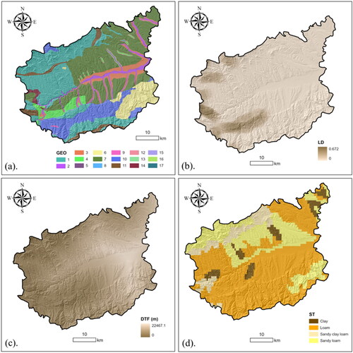
The study utilized several geological indicators for GWPM, including GEO, LD, DTF and ST (Figure 3). From the perspective of GEO, the groundwater storage is considerably influenced by geological features such as weathered products, source rocks, sediment conditions, hydraulic conductivity and porosity, and these structures can help in determining the existence of groundwater (Xie et al. 2014; Termeh et al. 2019). Within this research, geology was classified into 17 different classes, as shown in Supporting Information Table S2. Owing to the impacts of secondary porosity and permeability, higher values LD and lower values DTF are more likely to indicate groundwater occurrence, which indicates higher GWP (Falah et al. 2017). Additionally, GWP is affected by soil texture as it controls the infiltration of surface water into the groundwater system and influences the water holding capacity along with aquifer yield (Oh et al. 2011; Melese and Belay 2022).

Figure 3. Geological parameters. (a) GEO; (b) LD; (c) DTF; (d) ST.

3.1.3. Climate indicators

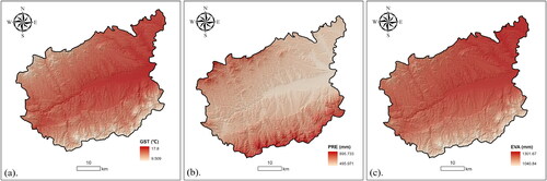
GST, PRE and EVA were selected as the climate indicators for GWPM in this study, and we selected the annual average data because of data availability (Figure 4). According to Mallick et al. (2015) and Wang et al. (2021), areas with lower GST are deemed to have higher GWP because groundwater has the ability to absorb heat from the ground surface. PRE is a significant indicator influencing the occurrence and recharge capacity of groundwater (Saranya and Saravanan 2020; Dar et al. 2021; Mosavi et al. 2021), which provides a large amount of water into aquifers through infiltration and increases groundwater levels (Jafari et al. 2019; Li et al. 2019; Abijith et al. 2020). EVA acts as an inverse indicator of PRE and can substantially decrease groundwater storage. Therefore, areas of high evaporation tend to exhibit lower GWP.

Figure 4. Climate parameters. (a) GST; (b) PRE; (c) EVA.

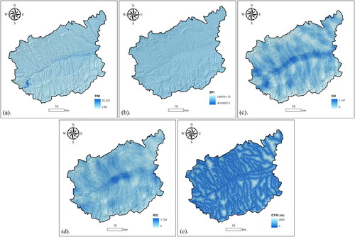
3.1.4. Hydrological indicators

TWI, SPI, DD, RID and DTRI were selected as hydrological indicators for this study (Figure 5). TWI describes the terrain profile that influences the water distribution accumulated in a point, subsequently affecting the storage of groundwater (Eq. (1)(1) $$\mathrm{TWI}=\ln \left(\frac{A_s}{\tan \beta }\right)$$(1) ) (Qadir et al. 2020). Thus, a higher TWI typically signifies higher GWP. SPI measures the erosive force of a stream, associated with to flow turbidity and infiltration (Golkarian and Rahmati 2018). Ahmad et al. (2020a) reported that the negative SPI values are beneficial for groundwater harnessing and indicate favorable areas for groundwater. The calculation of SPI is shown in Eq. (2)(2) $$\mathrm{SPI}=A_s\times \tan \beta$$(2) . Low DD implies high GWP because areas with low DD allow more time for water drainage and are susceptible to groundwater storage (Gupta and Srivastava 2010). Conversely, high DD areas are unfavorable for groundwater storage because the majority of groundwater might be rapidly lost through runoff (Hussein et al. 2017). Rivers are significant contributors to groundwater recharge, which affect the capability of spring formation (Chen et al. 2018). Areas with low river density and those distant from rivers rarely exhibit groundwater productivity (Rahmati and Melesse 2016). (1) $$\mathrm{TWI}=\ln \left(\frac{A_s}{\tan \beta }\right)$$(1) (2) $$\mathrm{SPI}=A_s\times \tan \beta$$(2) where $A_s$ is the specific catchment’s area and $\beta$ is the slope gradient.

Figure 5. Hydrological parameters. (a) TWI; (b) SPI; (c) DD; (d) RID; (e) DTRI.

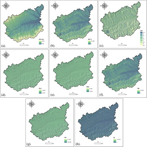
3.1.5. Topographic indicators

In this study, nine different topographic indicators were selected for GWPM, including ELE, SG, ASP, PLC, PRC, TRI, TPI and SL (Figure 6). Elevation can result in variations in climate conditions, soil classes and vegetation types, subsequently influencing groundwater conditions (Al-Abadi and Shahid 2015). Tahmassebipoor et al. (2016) highlighted that groundwater is typically abundant at low elevations but limited at very high elevations. Slope gradient impacts the infiltration and percolation of water into the ground because higher slopes augment flow speed, limiting the time for rainfall infiltration (Magesh et al. 2012). Aspect, a vital indicator, influences groundwater because it affects rainfall, wind direction, air moisture, vegetation and solar radiation (Zabihi et al. 2016). The curvature of topography determines flow properties, influencing the water infiltration process. PLC shows the flow divergence (positive value) or convergence (negative value) and PRC depicts the flow acceleration (positive value) or deceleration (negative value) (Ahmad et al. 2020b). TPI shows elevation values in comparison to surroundings, and it is rare to find high groundwater productivity in areas with high TPI due to steep topography (Mosavi et al. 2021). Consequently, GWP increases as TPI decrease. Likewise, TRI describes the topographic features by summing the variance of surroundings in elevation. A higher TRI value also represents lower GWP (Panahi et al. 2020). Lastly, SL provides an indication of potential soil loss likelihood from the perspective of slope properties through the combination of slope steepness and slope length (Das et al. 2022). A longer slope length may lead to a greater potential for groundwater recharge, as more water can percolate through the soil and reach the water table.

Figure 6. Topographic parameters. (a) ELE; (b) SG; (c) ASP; (d) PLC; (e) PRC; (f) TRI; (g) TPI; (h) SL.

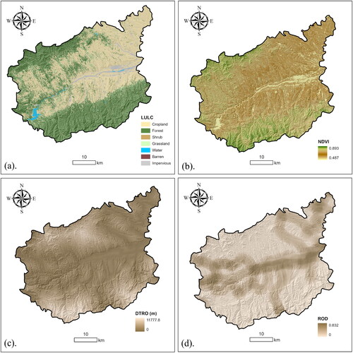
3.1.6. Land use and human activity indicators

LULC, NDVI, DTRO and ROD were selected as four indicators representing land use and human activity for GWPM in this study (Figure 7). LULC is a crucial indicator that may affect groundwater conditions due to its interaction with human activities and natural systems (Hasegawa et al. 2017). For example, groundwater usage in urban and agricultural areas is often intensive due to human activities, possibly reducing groundwater levels (Ahmad et al. 2020b). Moreover, the infiltration rates vary across different LULC types, which also may affect the GWP in an area (Al-Abadi et al. 2016). NDVI is a commonly used indicator to probe the relationship between water availability and vegetation (Fu and Burgher 2015). Higher NDVI values typically indicate a higher level of vegetation cover, usually associated with a higher GWP (Mallick et al. 2019). Road construction could induce alterations groundwater level and aquifer structures (Wang et al. 2022), and influences soil moisture and infiltration rates (Chen et al. 2020). Therefore, we selected the indicators of DTRO and RTD to assess GWP in the study area.

Figure 7. Land use and human activity parameters. (a) LULC; (b) NDVI; (c) DTRO; (d) ROD.

3.2. Description of models

Six ELMs were used for GWPM, including five BEMs (AdaBoost, GBDT, CatBoost, XGBoost and LightGBM) and a benchmark model (RF). All these models were implemented and executed within a Python environment, chosen for its versatility, rich library support and extensive community backing. In these models, hyperparameter space are important because it represents the range of values for various hyperparameters that control the behavior of the BEMs. Exploring this space is crucial for finding the optimal model configuration that maximizes performance. In this study, the determination of the hyperparameter space leans heavily on prior experience, and the meanings of hyperparameters in this study are shown in Supporting Information (Table S3).

3.2.1. RF

RF is a widely recognized and precise ELM that incorporates multiple decision trees for GWPM (Breiman 2001). It employs a bootstrap strategy to construct various decision trees with different subsets of the training data. This approach aids in mitigating overfitting, handling high-dimensional datasets and managing complex interactions during the modelling process (Al-Fugara et al. 2020). Specifically, the initial dataset is divided into two parts: in-bag samples (comprising 2/3 of the data) for training and out-of-bag (OOB) (comprising 1/3 of the data) samples for validation. The importance of parameters can be assessed by how much error increases when OOB data for that parameter is permuted (Naghibi et al. 2017a). The detailed procedures of RF are shown in Supporting Information (Section S1).

3.2.2. AdaBoost

AdaBoost is a popular nonparametric ensemble learning algorithm applicable to both classification and regression problems. It employs an adaptive re-sampling technique for selecting training samples (Tien Bui et al. 2016). Initially, in AdaBoost, a decision tree for training is created by assigning equal weights to the dataset. Then, higher weights are allocated to misclassified cases, while the weights of correctly classified cases remain unchanged. Once the normalization process completed, a new training subset is formed following the initial step until convergence criteria are met. Finally, AdaBoost is derived from a weighted sum of all classifiers (Chen et al. 2020). The detailed procedures of AdaBoost are shown in Supporting Information (Section S2).

3.2.3. GBDT

GBDT is an iterative decision tree algorithm, consisting of boosting as ensemble method and CART as the base classifier (Rong et al. 2023). It builds an ensemble of weak learners that are trained sequentially to improve the overall performance. GBDT can handle both numerical and categorical data and is applicable for both regression and classification tasks. During the iterative process, new decision trees are added to the ensemble, with each new tree trained to rectify the errors made by the previous trees. The weighted sum of all base classifiers determines the predicted result when GBDT converges, but the weights are not the same like in RF (Yang et al. 2023). The detailed procedures of GBDT refers to Supporting Information (Section S3).

3.2.4. CatBoost

CatBoost is a robust ML technique, which enables to handle the issues with noisy data, complex dependencies and heterogeneous features based on GBDT framework (Zhang et al. 2020). In this study, the training dataset is randomly sorted and the average label value for the same category is calculated and positioned before the given one in the permutation, which is called greedy target-based statistics (Greedy TS) strategy (Huang et al. 2019). The detailed procedures of CatBoost can be found in Supporting Information (Section S4). A notable shortcoming of this strategy is that features generally contain more information than targets. If the average value of labels is used to represent the features forcefully, a conditional shift may occur (Zhang et al. 2013). Thus, a straightforward approach to modify Greedy TS is to add a prior value $P.$ Suppose a dataset with samples $D=(x_i,Y_i),$ $i=1,\mathrm{ }2,.,\mathrm{ }n.$ If a random permutation is ${\sigma =(\sigma }_1,\mathrm{ }\dots ,\mathrm{ }{\sigma }_n),$ the calculation of the kth feature of pth data is defined as Eq. (3)(3) $$x_{p,k}=\frac{{\sum }_{j=1}^{p-1}\left[x_{{\sigma }_{j,k}}=x_{{\sigma }_{p,k}}\right]Y_{{\sigma }_j}+\beta P}{{\sum }_{j=1}^{p-1}[x_{{\sigma }_{j,k}}=x_{{\sigma }_{p,k}}]+\beta }$$(3) : (3) $$x_{p,k}=\frac{{\sum }_{j=1}^{p-1}\left[x_{{\sigma }_{j,k}}=x_{{\sigma }_{p,k}}\right]Y_{{\sigma }_j}+\beta P}{{\sum }_{j=1}^{p-1}[x_{{\sigma }_{j,k}}=x_{{\sigma }_{p,k}}]+\beta }$$(3) where $x_{i,k}$ is the $k\mathrm{th}$ feature of ith training sample, $Y_i$ is the target variable of the ith sample and $\beta$ is the weight of the prior value.

3.2.5. XGBoost

XGBoost is a supervised learning algorithm under the GBDT framework. It constructs a strong learner by combining multiple weak learners in parallel, thereby significantly increasing computational efficiency compared to conventional boosting methods. XGBoost employs a second-order Taylor expansion of the objective function during the tree construction process, which aids in effectively minimizing the loss function and improving model accuracy (Rasool et al. 2022). XGBoost incorporates a regularization technique to counteract overfitting issue and improve the generalization performance of a model. The regularized cost function of XGBoost algorithm is shown in Eq. (4)(4) $$L^{\left(t\right)}=\sum _{i=1}^{n}l(y_i,{\widehat{y}}_i^{\left(t-1\right)}+f_t(x_i\left)\right)+\Omega \left(f_t\right)$$(4) : (4) $$L^{\left(t\right)}=\sum _{i=1}^{n}l(y_i,{\widehat{y}}_i^{\left(t-1\right)}+f_t(x_i\left)\right)+\Omega \left(f_t\right)$$(4) where $t$ refers to the iteration numbers, $n$ is the total number of $y,$ $l$ is the loss function between actual value ($y_i$) and predicted value (${\widehat{y}}_i$), $x_i$ is the features of the $i\mathrm{th}$ sample, $f_t(x_i)$ represents the base learner added at the ith iteration and $\Omega (f_t)$ refers to additional regularization term to prevent overfitting. More detailed procedures about XGBoost calculation are shown in Supporting Information (Section S5).

3.2.6. LightGBM

LightGBM is a highly efficient and scalable algorithm under GBDT framework, which has seen extensive application for classification and regression tasks (Zhang et al. 2023). It incorporates gradient-based one-side sampling (GOSS) and exclusive feature bunding (EFB) to ensure the accuracy of both training and model prediction. GOSS enables to sample instances based on their gradients and improve training efficiency. Specifically, it performs a sampling process that keeps a large proportion of instances with high gradients and discards a small proportion of the instances with low gradients (Nafouanti et al. 2023). EFB can significantly reduce the dimensionality of the dataset and improve model performance while maintaining the interpretability of the model. Additionally, a leaf-wise technique is used to reduce overfitting issue and improve modeling speed and model performance. The procedures of LightGBM refer to Supporting Information (Section S6).

3.3. TPE hyperparameter optimization

Hyperparameter optimization plays a significant role in model performance and optimizing efficiency, which overcomes the shortcomings of the trial-and-error optimization approach. Bayesian optimization is a high-performance global optimization algorithm that uses previous sampling for the subsequent evaluations (Yu et al. 2022). TPE is a Bayesian optimization algorithm that uses a probabilistic model to search for optimal hyperparameters. To enhance the model performance in this study, we defined ‘1-area under receiver operating characteristic (AUROC) value’ as the objective function, aiming to finding the maximum AUROC for each model by calibration. The conditional probability $p(x|y)$ of TPE algorithm is defined as Eq. (5)(5) $$p\left(xy\right)=\{\begin{array}{c}l\left(x\right)\mathit{\text{ if y}}<y^{\mathrm{*}}\\ g\left(x\right)\mathit{\text{ if y}}\ge y^{\mathrm{*}}\end{array}$$(5) : (5) $$p\left(xy\right)=\{\begin{array}{c}l\left(x\right)\mathit{\text{ if y}}<y^{\mathrm{*}}\\ g\left(x\right)\mathit{\text{ if y}}\ge y^{\mathrm{*}}\end{array}$$(5) where $x$ is the hyperparameter, $y$ is the model loss, $y^{\mathrm{*}}$ refers to a threshold for loss based on data, $l\left(x\right)$ is probability density by using the loss function of the observation $x$ less than $y^{\mathrm{*}},$ and $g\left(x\right)$ denotes the probability density estimate of loss function of the observation $x$ greater than or equal to $y^{\mathrm{*}}.$ The expected improvement ($\mathrm{EI}$) is utilized for next evaluation to obtain an optimal effect on the objective value (Eq. (6)(6) $$\mathrm{E}{\mathrm{I}}_{y^{\mathrm{*}}}\left(x\right)={\int }_{\text{-}\mathrm{\infty }}^{y^{\mathrm{*}}}(y^{\mathrm{*}}-y)p\left(yx\right)dy={\int }_{\text{-}\mathrm{\infty }}^{y^{\mathrm{*}}}(y^{\mathrm{*}}-y)\frac{p\left(xy\right)p\left(y\right)}{p\left(x\right)}dy$$(6) ). (6) $$\mathrm{E}{\mathrm{I}}_{y^{\mathrm{*}}}\left(x\right)={\int }_{\text{-}\mathrm{\infty }}^{y^{\mathrm{*}}}(y^{\mathrm{*}}-y)p\left(yx\right)dy={\int }_{\text{-}\mathrm{\infty }}^{y^{\mathrm{*}}}(y^{\mathrm{*}}-y)\frac{p\left(xy\right)p\left(y\right)}{p\left(x\right)}dy$$(6)

Let $\gamma =p(y<y^{\mathrm{*}}),$ and Eqs. (7)(7) $$p\left(x\right)={\int }_{R}p\left(xy\right)p\left(y\right)dy=\gamma l\left(x\right)-(1-\gamma )g\left(x\right)$$(7) and (8)(8) $${\int }_{\text{-}\mathrm{\infty }}^{y^{\mathrm{*}}}\left(y^{\mathrm{*}}-y\right)p\left(xy\right)p\left(y\right)dy=\gamma y^{\mathrm{*}}l\left(x\right)-l\left(x\right){\int }_{\text{-}\mathrm{\infty }}^{y^{\mathrm{*}}}p\left(y\right)dy$$(8) can be constructed. (7) $$p\left(x\right)={\int }_{R}p\left(xy\right)p\left(y\right)dy=\gamma l\left(x\right)-(1-\gamma )g\left(x\right)$$(7) (8) $${\int }_{\text{-}\mathrm{\infty }}^{y^{\mathrm{*}}}\left(y^{\mathrm{*}}-y\right)p\left(xy\right)p\left(y\right)dy=\gamma y^{\mathrm{*}}l\left(x\right)-l\left(x\right){\int }_{\text{-}\mathrm{\infty }}^{y^{\mathrm{*}}}p\left(y\right)dy$$(8)

Therefore, $E{I}_{y^{\mathrm{*}}}\left(x\right)$ can be expressed as: (9) $$\mathrm{E}{\mathrm{I}}_{y^{\mathrm{*}}}\left(x\right)=\frac{\gamma y^{\mathrm{*}}l\left(x\right)-l\left(x\right){\int }_{\text{-}\mathrm{\infty }}^{y^{\mathrm{*}}}p\left(y\right)dy}{\gamma l\left(x\right)+(1-\gamma )g\left(x\right)}\propto {(\gamma +\frac{g\left(x\right)}{l\left(x\right)}(1-\gamma \left)\right)}^{-1}$$(9)

The maximum $\mathrm{EI}$ value can be obtained by constantly minimizing $g(x)/l(x)$ until the predetermined number of iterations. In this study, the iteration numbers were set as 1000.

3.4. GWPM and model validation

Using optimal hyperparameters from TPE, six GWP maps were generated under various ELMs. These maps were categorized into five levels using the natural breakpoint method: very high, high, moderate, low and very low GWP. To compare the model performances, this study selects field validation, positive predictive value (PPV) and ROC curve for model validation. Field validation qualitatively evaluates model performance using average well and borehole yield data for different GWP levels. PPV and ROC are statistical metrics for validating the performance of a model. Notably, some frequently used metrics like overall accuracy and negative predictive value were not considered in this study. The reason being, water managers are more focused on spring sites for sustainable groundwater use (Zabihi et al. 2016). Through model validation, we are able to derive the optimal model and the associated GWP map, which are invaluable resources for future sustainable groundwater management.

Four types of judgement results, including true positive (TP), true negative (TN), false positive (FP) and false negative (FN) are calculated. In this study, TP denotes accurate identification of spring locations by the model, whereas TN represents accurate non-spring locations indication. FP refers to incorrect prediction of spring locations, while FN signifies incorrect prediction of non-spring locations. The calculation of PPV, shown in Eq. (10)(10) $$\mathrm{PPV}=\frac{\mathrm{TP}}{\mathrm{TP}+\mathrm{FP}}$$(10) , is a combination of TP and FP, effectively fulfilling water managers’ needs for sustainable groundwater management. ROC curve is the most common and robust statistical metric in GWPM, and true positive rate (TPR) and false positive rate (FPR) are calculated by Eqs. (11)(11) $$\mathrm{TPR}=\frac{\mathrm{TP}}{\mathrm{TP}+\mathrm{FN}}$$(11) and (12)(12) $$\mathrm{FPR}=\frac{\mathrm{FP}}{\mathrm{TN}+\mathrm{FP}}$$(12) , and they are plotted in the coordinates for ROC curve creation (Xiong et al. 2023). (10) $$\mathrm{PPV}=\frac{\mathrm{TP}}{\mathrm{TP}+\mathrm{FP}}$$(10) (11) $$\mathrm{TPR}=\frac{\mathrm{TP}}{\mathrm{TP}+\mathrm{FN}}$$(11) (12) $$\mathrm{FPR}=\frac{\mathrm{FP}}{\mathrm{TN}+\mathrm{FP}}$$(12)

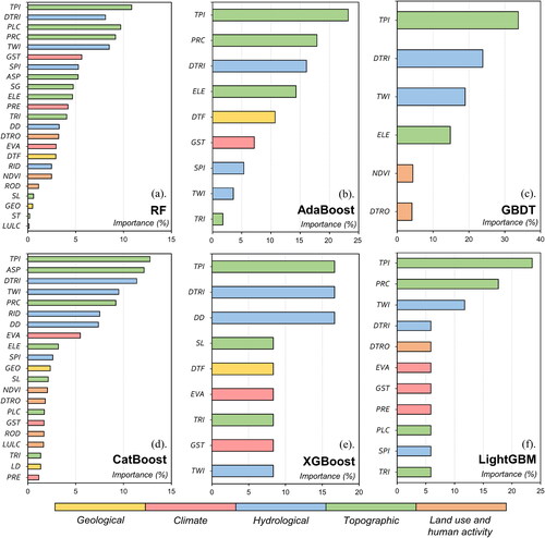
3.5. Indicator importance analysis and spatial correlation

The importance of different indicators can be obtained from the ELMs, which represents the extent to which these indicators contributed to the model’s formulation. We derived the indicator importance for each model and standardized them using Eq. (13)(13) $${\mathrm{PI}}_{i\text{-}\mathrm{standard}}=\frac{{\mathrm{PI}}_i}{{\mathrm{PI}}_1+{\mathrm{PI}}_2+\dots +{\mathrm{PI}}_n}$$(13) . (13) $${\mathrm{PI}}_{i\text{-}\mathrm{standard}}=\frac{{\mathrm{PI}}_i}{{\mathrm{PI}}_1+{\mathrm{PI}}_2+\dots +{\mathrm{PI}}_n}$$(13) where ${\mathrm{PI}}_{i\text{-}\mathrm{standard}}$ is the standard form of the importance of indicator $i,$ ${\mathrm{PI}}_i$ is the output of the importance of indicator $i$ and $n$ is the number of indicators.

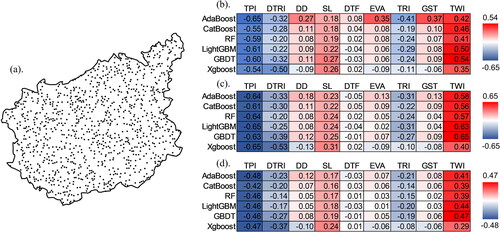
ELMs (including many ML models) generally strive for superior model performance, with limited regard to the positive or negative influences of indicators on GWP prediction. To ascertain if the optimal model accurately predicts the correlations as illustrated in Subsection 3.1, a test of spatial correlation between indicators and the GWP map is necessary. The steps are as follows: (a). Randomly generate 1000 points within the study area; (b). For each random point, extract the value of each indicator and the probability of GWP in different models; (c). Test the correlations between indicators and GWPs using different correlation coefficients, including Pearson correlation coefficient ($r_{xy}$) (Eq. (14)(14) $$r_{xy}=\frac{n\sum x_i{y}_i-\sum x_i\sum y_i}{\sqrt{n\sum x_i^2-{\left(\sum x_i\right)}^2}\sqrt{n\sum y_i^2-{\left(\sum y_i\right)}^2}}$$(14) ), Spearman rank correlation coefficient ($\rho$) (Eq. (15)(15) $$\rho =1-\frac{6\sum d_i^2}{n(n^2-1)}$$(15) ) and Kendall correlation coefficient ($\tau$) (Eq. (16)(16) $$\tau =\frac{n_c-n_d}{\frac{1}{2}n(n-1)}$$(16) ). (14) $$r_{xy}=\frac{n\sum x_i{y}_i-\sum x_i\sum y_i}{\sqrt{n\sum x_i^2-{\left(\sum x_i\right)}^2}\sqrt{n\sum y_i^2-{\left(\sum y_i\right)}^2}}$$(14) (15) $$\rho =1-\frac{6\sum d_i^2}{n(n^2-1)}$$(15) (16) $$\tau =\frac{n_c-n_d}{\frac{1}{2}n(n-1)}$$(16) where $x_i$ is the value of $x$ for $i\mathrm{th}$ observation, $y_i$ is the value of $y$ for $i\mathrm{th}$ observation, $n$ is the number of observations, $d_i$ is the difference between the ranks of corresponding variables, $n_c$ is the number of concordant and $n_d$ is the number of discordant.

4. Results and discussion

4.1. Optimal hyperparameters and GWPM

Table 3 shows the hyperparameter optimization results calibrated by TPE for different models. Based on these hyperparameters, six GWP maps are generated, as shown in Figure 8. Table 4 provides a summary of the area distribution for different GWP levels. Although the six models produce distinct GWP map patterns and differing areas under various groundwater levels, visual inspection reveals that the regions with high groundwater potential tend to follow a belt-like shape, closely aligned with the river’s path. However, when comparing the ‘very high GWP’ areas predicted by AdaBoost and XGBoost models, interesting differences emerge. The XGBoost model depicts very high GWP areas as a river buffered on both sides, whereas the AdaBoost model indicates more concentrated potential in the central and northern parts of the study area. These variations highlight the different interpretations and emphasis on spatial attributes by distinct models. The validation dataset, including 20 spring points and 20 non-spring points has been shown on Figure 8. Visually, the model suggests a higher concentration of springs in areas marked in dark blue, while lighter-shaded areas seem to contain more non-spring points, indicating a certain level of rationality in the model’s GWPM. A detailed discussion regarding the performance of these models is provided in the subsequent section.

Figure 8. GWP maps. (a) RF; (b) AdaBoost; (c) GBDT; (d) CatBoost; (e) XGBoost; (f) LightGBM.

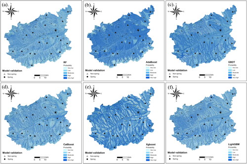
Table 3. Hyperparameter optimization results of different models.

Model	Hyperparameters	Hyperparameter space	Optimum
RF	n_estimators	hp.choice('n_estimators’,range(1,500))	10
	max_depth	hp.choice('max_depth’,range(1,20))	10
	min_samples_leaf	hp.choice('min_samples_leaf’,range(1,5))	2
AdaBoost	n_estimators	hp.choice('n_estimators’,range(1,500))	56
	learning_rate	hp.uniform('learning_rate’, 0.01, 0.5)	0.0659
	algorithm	hp.choice('algorithm’, ['SAMME', 'SAMME.R'])	SAMME.R
GBDT	num_leaves	hp.choice(‘num_leaves’,range(15,128))	46
	learning_rate	hp.uniform('learning_rate’, 0.01, 0.5)	0.4160
	bagging_freq	hp.choice(‘bagging_freq’,range(4,7))	4
	bagging_fraction	hp.uniform('bagging_fraction’, 0.5, 0.9)	0.6002
	feature_fraction	hp.uniform('feature_fraction’, 0.5, 0.9)	0.5893
CatBoost	learning_rate	hp.uniform('learning_rate’, 0.01, 0.5)	0.2598
	depth	hp.choice('depth’, range(3, 12))	7
	l2_leaf_reg	hp.loguniform('l2_leaf_reg’, −3, 5)	2.7504
	iterations	hp.choice('iterations’, range(100, 1000, 100))	500
	border_count	hp.choice('border_count’, range(32, 256, 32))	224
XGBoost	eta	hp.uniform(‘eta’, 0.001,0.5)	0.3165
	gamma	hp.uniform(‘gamma’, 0.1,0.5)	0.1478
	max_depth	hp.choice(‘max_depth’, [2,3,4,5,6,7,8,9,10])	5
	min_child_weight	hp.choice(‘min_child_weight’, [1,2,3,4,5,6,7,8])	2
	reg_alpha	hp.choice(‘reg_alpha’, [0,0.01,0.05,0.1,0.5])	0.05
	subsample	hp.uniform(‘subsample’, 0,0.9)	0.3809
LightGBM	bagging_fraction	hp.uniform('bagging_fraction’, 0.5, 0.9)	0.6002
	bagging_freq	hp.choice(‘bagging_freq’, range(4,7))	4
	feature_fraction	hp.uniform('feature_fraction’, 0.5, 0.9)	0.5893
	learning_rate	hp.uniform('learning_rate’, 0.01, 0.5)	0.4160
	num_leaves	hp.choice(‘num_leaves’, range(15,128))	46

Table 4. Areas of GWP levels in different models.

GWP levels	RF	AdaBoost	GBDT	CatBoost	XGBoost	LightGBM
Very low (km^2)	437.47	107.31	88.15	448.28	1.06	538.20
Low (km^2)	539.84	293.43	360.26	544.10	262.63	439.07
Moderate (km^2)	558.74	437.51	711.86	523.82	908.68	425.12
High (km^2)	508.86	438.14	575.72	474.23	267.80	503.27
Very High (km^2)	258.35	1026.88	567.28	312.85	863.11	538.20

4.2. Model validation and comparisons

Table 5 shows the average yields (L/s) of wells and boreholes across various levels of GWP as validated in the field for six different models. In general, a consistent trend is observable across all six models: the average yield increases from areas with very low GWP to those with very high GWP, validating the logicality and efficacy of these models. Notably, a significant proportion of wells and boreholes are situated within very high GWP areas. The average yields of XGBoost (13.2727 L/s), LGBM (13.8267 L/s) and CatBoost (12.9909 L/s) models within these zones surpass the yields predicted by the other models, indicating the exceptional performance of these three models in GWP prediction for very high GWP areas. In high GWP areas, the results derived from the six models display a substantial difference, with RF model showing a peak yield of 15.1999 L/s. However, this finding may be inconclusive due to its derivation from a single data point. For the remaining regions, the models demonstrate similar performance through field validation. The accuracy and robustness of XGBoost, LGBM and CatBoost models in predicting high GWP areas are likely attributable to their advanced boosting algorithms, which minimize bias and overfitting. This contributes to their superiority in predicting high GWP regions, providing valuable insights for groundwater management.

Table 5. Field validation results.

Model	Levels	Number of wells/boreholes	Average yields (L/s)
XGBoost	Very low GWP areas	0	/
	Low GWP areas	6	0.9852
	Moderate GWP areas	4	2.3589
	High GWP areas	2	0.4110
	Very high GWP areas	10	13.2727
LGBM	Very low GWP areas	0	/
	Low GWP areas	3	2.7773
	Moderate GWP areas	5	0.7534
	High GWP areas	7	5.7157
	Very high GWP areas	7	13.8267
CatBoost	Very low GWP areas	0	/
	Low GWP areas	2	2.4989
	Moderate GWP areas	8	0.7924
	High GWP areas	2	3.8250
	Very high GWP areas	10	12.9909
GBDT	Very low GWP areas	0	/
	Low GWP areas	0	/
	Moderate GWP areas	6	1.6238
	High GWP areas	10	7.3416
	Very high GWP areas	6	10.9561
AdaBoost	Very low GWP areas	0	/
	Low GWP areas	1	0.0401
	Moderate GWP areas	5	1.8280
	High GWP areas	2	2.0879
	Very high GWP areas	14	9.6814
RF	Very low GWP areas	1	3.3078
	Low GWP areas	4	1.2847
	Moderate GWP areas	7	6.0477
	High GWP	1	15.1999
	Very high GWP	9	9.2127

Figure 9 depicts the outcomes of the ROC curve and additional predictive metrics, providing a more quantitative evaluation that basically aligns with the results of the field validation. Generally, the AUROC values for the six ELMs range from 0.734 to 0.900, which indicates ‘good’ to ‘excellent’ model performance in GWMP (Naghibi et al. 2017a). Compared to the benchmark model, AdaBoost underperforms in terms of PPV and AUROC values, while other BEMs surpass the performance of RF to varying degrees. With its PPV and AUROC scores nearing 0.9, the XGBoost model emerges as the top performer, outshining the majority of ML models in GWPM (Thanh et al. 2022). Among the 11 spring that were considered by the XGBoost model, there was only one misprediction. Nevertheless, the highest FN value among the six models indicates that the XGBoost model’s prediction of non-spring points lacks precision, but this is less crucial in the context of GWPM. The superior performance of XGBoost model has been affirmed in a variety of environmental applications, such as landslide susceptibility prediction (Can et al. 2021), daily streamflow prediction (Szczepanek 2022), landslide dam stability (Shi et al. 2022), groundwater levels (Osman et al. 2021), groundwater contamination (Nafouanti et al. 2023) and bench water quality (Li et al. 2022). Our study adds to the growing body of evidence supporting the effectiveness and efficiency of the XGBoost model for GWMP.

Figure 9. Model validation results. (a) RF; (b) AdaBoost; (c) GBDT; (d) CatBoost; (e) XGBoost; (f) LightGBM.

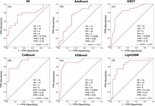
Following XGBoost, CatBoost model also shows strong performance (AUROC = 0.900, PPV = 0.75). However, as a newer BEM, the performance of LightGBM falls short of XGBoost and CatBoost and does not surpass GBDT, diverging from the field validation results. In LightGBM, the histogram-based algorithm significantly increased model efficiency in determining split points during tree growth. However, the increase in model efficiency comes with a decrease in some instances with small gradients and a reduction in feature numbers, which may marginally compromise the prediction accuracy in LightGBM (Naghibi et al. 2017a). Interestingly, although the AUROC value of CatBoost exceeds that of GBDT, its PPV is lower. This inconsistency also appears in RF and LightGBM. While this discrepancy does not affect the selection of the optimal model (XGBoost) in this study, it suggests that defining the objective function as the minimum ‘1-AUROC’ may not be the most suitable approach. Therefore, it is crucial to realize that while the XGBoost model outperforms others in this study, the selection and optimization of BEMs for GWPM should be context-specific.

4.3. Indicator importance analysis

Despite the absence of a universally accepted set of indicators for GWPM, the capability of ELMs to determine the important indicators is a significant advantage (Termeh et al. 2019; Pham et al. 2021). Figure 10 shows the indicator importance for six models, highlighting the significance of TPI, DTRI and TWI in GWPM in the study area. Notably, the importance of TPI is prominent, exceeding 30% in the GBDT model, surpassing 20% in AdaBoost and LGBM, and going beyond 10% in the remaining three models. Furthermore, as illustrated in Figure 10, topographic and hydrological indicators stand out as the most dominant categories, with the green and blue bars consistently occupying the top rankings. Comparing these results with current studies reveals some key insights. Conventionally, higher TPI values signify increased surface runoff and diminished infiltration, potentially impacting groundwater recharge substantially (Mukherjee and Singh 2020). However, despite TPI being used as a GWP assessment indicator in some literature such as Yadav et al. (2023), Mosavi et al. (2021) and Fatema et al. (2023), it seems that its significance is currently underappreciated in GWPM. The significance of DTRI and TWI, highlighted in various studies (Zabihi et al. 2016; Mousavi et al. 2017; Golkarian et al. 2018; Naghibi et al. 2020), along with the proven significance of topographic and hydrological indicators in GWPM (Naghibi et al. 2016, 2018; Davoudi Moghaddam et al. 2020), emphasized the need for attention to these indicators. In a compelling example, Naghibi et al. (2020) exclusively employed 13 DEM-derived indicators (including topographic and hydrological indicators) to assess GWP, achieving AUROC values of approximately 0.85. Notwithstanding, variations in indicator significance are observable in areas with predominantly flat land well or spring distribution including regions with sparse well or spring distribution in mountainous areas (Chen et al. 2019; Chen and Zhang 2021; Saha et al. 2022). In such studies, indicators like GEO, NDVI, LULC, ST and geomorphology may hold greater importance. Additionally, in arid or semi-arid regions, climate factors such as PRE and EVA play a role in GWPM (Gomez-Escalonilla et al. 2022; Wang et al. 2022; Guo et al. 2023a). In mountainous areas, the steep slopes and rugged terrain promotes rapid water flow downhill, inducing highly variable groundwater conditions. Conversely, in plains areas with more consistent water flow, infiltration-associated factors such as GEO, LULC and ST become more significant. In arid or semi-arid environments, low PER and high EVA largely govern groundwater conditions. Notably, due to their role as significant groundwater recharge sources, rivers remain an unignorable element for GWPM, explaining the frequent high rank of DTRI in many studies (Zabihi et al. 2016; Das and Saha 2022). Therefore, this study highlights the importance of context in selecting GWP indicators, emphasizing the adaptive capabilities of ELMs, particularly XGBoost, for optimizing performance. Also, our results advocate for focused attention on topographic and hydrological indicators, especially TPI, DTRI and TWI, as crucial contributors to effective GWPM in mountainous regions.

Figure 10. Importance analysis of indicators. (a) RF; (b) AdaBoost; (c) GBDT; (d) CatBoost; (e) XGBoost; (f) LightGBM.

4.4. Correlation analysis of important indicators

Figure 11 depicts the correlation coefficients between nine indicators and the GWPs within the XGBoost model. This verifies the accuracy of correlations utilized by the optimal model between indicators and GWPs during the modelling process. Figure 11a presents the locations of 1000 points selected randomly in the study area, and Figure 11b–d show the correlation coefficients of Pearson, Spearman and Kendall across different models respectively. According to Figure 11, the distributions of TPI (–0.48 to −0.65), DTRI (–0.14 to −0.53) and TWI (0.29 to 0.65) maintain relatively strong correlations with GWPs in all models, aligning with the indicator importance analysis. Comparison with the empirical impacts of indicators on GWPs reveals accurate predictions of correlations for TPI, DTRI, SL, TRI and TWI. However, slight inconsistencies appear for indicators DD, GST, EVA and DTF. Theoretically, high DD implies reduced infiltrating water due to lower permeability (Ahmed et al. 2015), a correlation that XGBoost captures accurately, unlike other models. Similar issue arises with the GST and EVA indicators. Empirically, high GST and EVA tend to imply lower GWP (Mallick et al. 2015; Wang et al. 2021), and XGBoost also accurately forecasted the correlations. These accurate predictions underscore the superior performance of the XGBoost model compared to the other models. However, regarding DTF, the correlation is insignificant in XGBoost model and other models also devalue this indicator. These variations likely stem from intricate interactions among indicators, suggesting the existence of a complex interplay of factors affecting GWPs. The XGBoost model’s success in accurately predicting correlations between essential indicators and GWPs underscores its robustness and capability to capture these nuanced relationships, resonating closely with empirical insights. Investigating these interactions further and refining models to account for these connections could lead to better GWPM, contributing to more informed and sustainable groundwater management.

Figure 11. Correlation analysis of important indicators. (a) Random points; (b) Pearson correlation coefficient result; (c) Spearman correlation coefficient result; (d) Kendall correlation coefficient result.

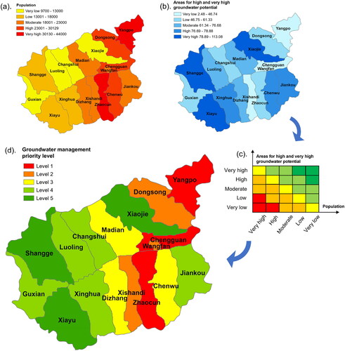
4.5. Sustainable groundwater management

Groundwater, as a crucial water resource, requires effective and sustainable management that takes into account human demands. Figure 12 shows how the GWP map supports sustainable groundwater management in the study area. Figure 12a shows the distribution of population in different townships of Luoning County, which indicates the groundwater demands of each township. Figure 12b displays the areas for high and very GWP created by XGBoost, which indicate available groundwater supply. We then synthesized these two elements into a matrix (Figure 12c) and devised a groundwater management priority map (Figure 12d), which can be used for proposing strategies of varying levels. Based on Figure 12d, we proposed an example of sustainable groundwater management strategies, with differing priority levels for different townships in Luoning County (Supporting Information Table S3), with strategy intensity waning from priority level 1 to 5. Yangpo, Chengguan and Zhaocun hold priority level 1, warranting immediate attention and prioritization of comprehensive measures. It is essential to note that GWPM serves as the preliminary stage for sustainable groundwater management. Subsequent works may include sustainable groundwater exploitation, water resource allocation, groundwater conservation, water policy adjustments and reforms, land use management and water-efficient practice promotion. Currently, integrating GWP maps into sustainable groundwater management under the framework of the Sustainable Development Goals (SDGs) remains a considerable challenge. Hence, we highly recommend researchers to extend their GWP studies beyond high-performance model development and investigate practical applications for sustainable groundwater management, fostering progress towards the SDGs.

Figure 12. The determination of groundwater management priority levels. (a) Population distribution; (b) Areas for high and very high GWP; (c) The matrix for the combination of population and GWP map; (d) Groundwater management priority levels in Luoning County.

4.6. Limitations, suggestions and future research

This research is subject to three limitations. Firstly, the inconsistency in the scale of the indicators, with some having a resolution of 30 m and others 1 km, could potentially impact the precision of the results. Secondly, the dataset used in this study is relatively limited in size, comprising 97 spring data points, of which 77 were utilized for training and 20 for validation. Despite a preliminary analysis has been conducted for the split of training and validation sets, a degree of uncertainty remains. Lastly, ‘1-AUC’ defined in this study may not be the most effective objective function. It only takes into account the optimality of a single metric, neglecting other potential factors. Despite these limitations, the findings and conclusions drawn from this study are still significant for GWPM and sustainable groundwater management. In terms of suggestions and future research, firstly, our work highlights the potential of ELMs and BEMs in improving model performance in GWPM, especially when using XGBoost. We suggest further investigation into ELMs to improve prediction accuracy and foster the advancement of GWPM. Secondly, while this study defined the minimum ‘1-AUC’ as the loss function to obtain optimal parameters, it may not be the most effective approach. The evaluation metrics for a GWPM model should be more intricate and comprehensive, encompassing not only statistical metrics such as AUROC and PPV, computing efficiency and management guidance ability. Thus, we recommend employing a more comprehensive and complex system to assess model performance. Thirdly, while TPI was identified as a crucial indicator in this study, it is seldom mentioned in existing literature. Given the lack of a universal consensus on indicator selection in GWPM, we propose that TPI, DTRI and TWI, along with additional topographic and hydrological indicators, should be thoroughly considered for GWPM in mountainous regions. Concurrently, we encourage the development of a more standardized indicator system for more accurate GWP prediction. Fourthly, a notable drawback is that many ELMs primarily aim for superior model performance, often overlooking the positive or negative impacts of indicators on GWP prediction. Consequently, future research endeavors should consider investigating methods to mitigate the influence of these inconsistencies on the model. Lastly, as GWPM serves as the preliminary stage for sustainable groundwater management, we urge future research on GWP to focus more on the application of GWPM for sustainable groundwater management, as shown in this study.

5. Conclusion

Groundwater, an important natural resource, plays a vital role in supporting economic, social and environmental development, and GWPM offers invaluable insights into the volume of groundwater that can be extracted from an aquifer without adversely affecting groundwater yield and environmental conditions. Given the current insufficient application of ELMs, especially for BEMs, and the incomplete construction of the indicator system in GWPM, this study employed six ELMs, TPE hyperparamter optimization method and 24 indicators for GWPM by taking Luoning County, China as the case study. These models include five BEMs (AdaBoost, GBDT, CatBoost, XGBoost and LightGBM) that have not been previously applied or evaluated in GWPM, along with one benchmark model (RF). The primary findings are as follows.

The six models create different GWP map patterns, and areas under various groundwater levels also differ. Based on field validation and two statistical metrics (ROC curve and PPV), XGBoost demonstrated the superior model performance, trailed by CatBoost, GBDT and LightGBM. The performances of RF and AdaBoost were comparatively lower. Indicator correlation analysis revealed that XGBoost could essentially predict the correlations between the crucial indicators and GWPs, without significant inconsistency in relation to experience, thereby outperforming other models. TPI, DTRI and TWI emerged as the three most significant indicators across all models. The topographic and hydrological indicators constituted two crucial indicator groups in this research. It fully reflects the importance of topographic and hydrological indicators in GWPM in mountainous areas. The ability of ELMs to determine the important indicators to achieve superior model performance is a significant advantage, and its promotion in GWPM is highly recommended. The townships of Luoning County were categorized into five levels to implement varying levels of sustainable groundwater management strategies, with Yangpo, Chengguan and Zhaocun receiving the highest priority. The method of transitioning from a GWP map to sustainable groundwater management priority is deemed worthy of promotion. Although this article has the limitations of data scale, data size and objective function determination, the findings and conclusions drawn are still significant for GWPM development and sustainable groundwater management. Finally, this study proposes five specific suggestions for future research. These include exploring the application of ELMs in GWPM, constructing a more comprehensive model performance evaluation system, establishing a more standardized indicator system, developing methods to mitigate the influence of inconsistencies between indicators and prediction results, and expanding the application of GWPM for sustainable groundwater management.

Disclosure statement

The authors declare that they have no known competing financial interests or personal relationships that could have appeared to influence the work reported in this article.

Data availability

The authors do not have permission to share data.

Additional information

Funding

This work was financially supported by the National Natural Science Foundation of China (No. 41572212).

References

- Abedi R, Costache R, Shafizadeh-Moghadam H, Pham QB. 2022. Flash-flood susceptibility mapping based on XGBoost, random forest and boosted regression trees. Geocarto Int. 37(19):5479–5496. doi: 10.1080/10106049.2021.1920636.
- Abijith D, Saravanan S, Singh L, Jennifer JJ, Saranya T, Parthasarathy K. 2020. GIS-based multi-criteria analysis for identification of potential groundwater recharge zones-a case study from Ponnaniyaru watershed, Tamil Nadu, India. HydroResearch. 3:1–14. doi: 10.1016/j.hydres.2020.02.002.
- Ahmad I, Dar MA, Andualem TG, Teka AH. 2020a. Groundwater development using geographic information system. Appl Geomat. 12(1):73–82. doi: 10.1007/s12518-019-00283-6.
- Ahmad I, Dar MA, Teka AH, Teshome M, Andualem TG, Teshome A, Shafi T. 2020b. GIS and fuzzy logic techniques-based demarcation of groundwater potential zones: a case study from Jemma River basin, Ethiopia. J Afr Earth Sci. 169:103860. doi: 10.1016/j.jafrearsci.2020.103860.
- Ahmed K, Shahid S, Bin Harun S, Ismail T, Nawaz N, Shamsudin S. 2015. Assessment of groundwater potential zones in an arid region based on catastrophe theory. Earth Sci Inform. 8(3):539–549. doi: 10.1007/s12145-014-0173-3.
- Al-Abadi AM, Al-Temmeme AA, Al-Ghanimy MA. 2016. A GIS-based combining of frequency ratio and index of entropy approaches for mapping groundwater availability zones at Badra–Al Al-Gharbi–Teeb areas, Iraq. Sustain Water Resour Manag. 2(3):265–283. doi: 10.1007/s40899-016-0056-5.
- Al-Abadi AM, Fryar AE, Rasheed AA, Pradhan B. 2021. Assessment of groundwater potential in terms of the availability and quality of the resource: a case study from Iraq. Environ Earth Sci. 80(12):1–22.
- Al-Abadi AM, Shahid S. 2015. A comparison between index of entropy and catastrophe theory methods for mapping groundwater potential in an arid region. Environ Monit Assess. 187(9):576. doi: 10.1007/s10661-015-4801-2.
- Al-Fugara A, Pourghasemi HR, Al-Shabeeb AR, Habib M, Al-Adamat R, Ai-Amoush H, Collins AL. 2020. A comparison of machine learning models for the mapping of groundwater spring potential. Environ Earth Sci. 79(10):19.
- Amade N, Painho M, Oliveira T. 2018. Geographic information technology usage in developing countries - a case study in Mozambique. Geo-Spat Inf Sci. 21(4):331–345. doi: 10.1080/10095020.2018.1523995.
- Breiman L. 2001. Random forests. Mach Learn. 45(1):5–32. doi: 10.1023/A:1010933404324.
- Can R, Kocaman S, Gokceoglu C. 2021. A comprehensive assessment of XGBoost algorithm for landslide susceptibility mapping in the upper basin of Ataturk dam, Turkey. Appl Sci. 11(11):4993. doi: 10.3390/app11114993.
- Chen T, Guestrin C. 2016. Xgboost: a scalable tree boosting system; p. 785–794.
- Chen W, Li H, Hou E, Wang S, Wang G, Panahi M, Li T, Peng T, Guo C, Niu C, et al. 2018. GIS-based groundwater potential analysis using novel ensemble weights-of-evidence with logistic regression and functional tree models. Sci Total Environ. 634:853–867. doi: 10.1016/j.scitotenv.2018.04.055.
- Chen W, Panahi M, Khosravi K, Pourghasemi HR, Rezaie F, Parvinnezhad D. 2019. Spatial prediction of groundwater potentiality using ANFIS ensembled with teaching-learning-based and biogeography-based optimization. J Hydrol. 572:435–448. doi: 10.1016/j.jhydrol.2019.03.013.
- Chen W, Zhao X, Tsangaratos P, Shahabi H, Ilia I, Xue W, Wang X, Ahmad BB. 2020. Evaluating the usage of tree-based ensemble methods in groundwater spring potential mapping. J Hydrol. 583:124602. doi: 10.1016/j.jhydrol.2020.124602.
- Chen WW, Zhang S. 2021. GIS-based comparative study of Bayes network, Hoeffding tree and logistic model tree for landslide susceptibility modeling. Catena. 203:105344. doi: 10.1016/j.catena.2021.105344.
- Chen Y, Chen W, Chandra Pal S, Saha A, Chowdhuri I, Adeli B, Janizadeh S, Dineva AA, Wang X, Mosavi A. 2022. Evaluation efficiency of hybrid deep learning algorithms with neural network decision tree and boosting methods for predicting groundwater potential. Geocarto Int. 37(19):5564–5584. doi: 10.1080/10106049.2021.1920635.
- Chowdhury A, Jha M, Chowdary V, Mal B. 2009. Integrated remote sensing and GIS‐based approach for assessing groundwater potential in West Medinipur district, West Bengal, India. Int J Remote Sens. 30(1):231–250. doi: 10.1080/01431160802270131.
- Dar T, Rai N, Bhat A. 2021. Delineation of potential groundwater recharge zones using analytical hierarchy process (AHP). Geol Ecol Landsc. 5(4):292–307. doi: 10.1080/24749508.2020.1726562.
- Das R, Saha S. 2022. Spatial mapping of groundwater potentiality applying ensemble of computational intelligence and machine learning approaches. Groundw Sustain Dev. 18:100778. doi: 10.1016/j.gsd.2022.100778.
- Das S, Bora PK, Das R. 2022. Estimation of slope length gradient (LS) factor for the sub-watershed areas of Juri River in Tripura. Model Earth Syst Environ. 8(1):1171–1177. doi: 10.1007/s40808-021-01153-0.
- Davoudi Moghaddam D, Rahmati O, Haghizadeh A, Kalantari Z. 2020. A modeling comparison of groundwater potential mapping in a mountain bedrock aquifer: QUEST, GARP, and RF models. Water. 12(3):679. doi: 10.3390/w12030679.
- Falah F, Ghorbani Nejad S, Rahmati O, Daneshfar M, Zeinivand H. 2017. Applicability of generalized additive model in groundwater potential modelling and comparison its performance by bivariate statistical methods. Geocarto Int. 32(10):1069–1089. doi: 10.1080/10106049.2016.1188166.
- Fatema K, Joy MAR, Amin FR, Sarkar SK. 2023. Groundwater potential mapping in Jashore, Bangladesh. Heliyon. 9(3):e13966. doi: 10.1016/j.heliyon.2023.e13966.
- Freund Y, Schapire RE. 1997. A decision-theoretic generalization of on-line learning and an application to boosting. J Comput Syst Sci. 55(1):119–139. doi: 10.1006/jcss.1997.1504.
- Friedman JH. 2001. Greedy function approximation: a gradient boosting machine. Ann Stat. 29:1189–1232.
- Fu B, Burgher I. 2015. Riparian vegetation NDVI dynamics and its relationship with climate, surface water and groundwater. J Arid Environ. 113:59–68. doi: 10.1016/j.jaridenv.2014.09.010.
- Gambella C, Ghaddar B, Naoum-Sawaya J. 2021. Optimization problems for machine learning: a survey. Eur J Oper Res. 290(3):807–828. doi: 10.1016/j.ejor.2020.08.045.
- Gaye CB, Tindimugaya C. 2019. Challenges and opportunities for sustainable groundwater management in Africa. Hydrogeol J. 27(3):1099–1110. doi: 10.1007/s10040-018-1892-1.
- Golkarian A, Naghibi SA, Kalantar B, Pradhan B. 2018. Groundwater potential mapping using C5. 0, random forest, and multivariate adaptive regression spline models in GIS. Environ Monit Assess. 190(3):149. doi: 10.1007/s10661-018-6507-8.
- Golkarian A, Rahmati O. 2018. Use of a maximum entropy model to identify the key factors that influence groundwater availability on the Gonabad Plain, Iran. Environ Earth Sci. 77:1–20.
- Gomez-Escalonilla V, Martinez-Santos P, Martin-Loeches M. 2022. Preprocessing approaches in machine-learning-based groundwater potential mapping: an application to the Koulikoro and Bamako regions, Mali. Hydrol Earth Syst Sci. 26(2):221–243. doi: 10.5194/hess-26-221-2022.
- Green TR, Taniguchi M, Kooi H, Gurdak JJ, Allen DM, Hiscock KM, Treidel H, Aureli A. 2011. Beneath the surface of global change: impacts of climate change on groundwater. J Hydrol. 405(3–4):532–560. doi: 10.1016/j.jhydrol.2011.05.002.
- Guo X, Gui X, Xiong H, Hu X, Li Y, Cui H, Qiu Y, Ma C. 2023a. Critical role of climate factors for groundwater potential mapping in arid regions: insights from random forest, XGBoost, and LightGBM algorithms. J Hydrol. 621:129599. doi: 10.1016/j.jhydrol.2023.129599.
- Guo X, Xiong H, Li H, Gui X, Hu X, Li Y, Cui H, Qiu Y, Zhang F, Ma C. 2023b. Designing dynamic groundwater management strategies through a composite groundwater vulnerability model: integrating human-related parameters into the DRASTIC model using LightGBM regression and SHAP analysis. Environ Res. 236(Pt 2):116871. doi: 10.1016/j.envres.2023.116871.
- Gupta M, Srivastava PK. 2010. Integrating GIS and remote sensing for identification of groundwater potential zones in the hilly terrain of Pavagarh, Gujarat, India. Water Int. 35(2):233–245. doi: 10.1080/02508061003664419.
- Hamed Y, Hadji R, Redhaounia B, Zighmi K, Bâali F, El Gayar A. 2018. Climate impact on surface and groundwater in North Africa: a global synthesis of findings and recommendations. Euro-Mediterr J Environ Integr. 3(1):1–15. doi: 10.1007/s41207-018-0067-8.
- Hasegawa T, Fujimori S, Ito A, Takahashi K, Masui T. 2017. Global land-use allocation model linked to an integrated assessment model. Sci Total Environ. 580:787–796. doi: 10.1016/j.scitotenv.2016.12.025.
- Huang G, Wu L, Ma X, Zhang W, Fan J, Yu X, Zeng W, Zhou H. 2019. Evaluation of CatBoost method for prediction of reference evapotranspiration in humid regions. J Hydrol. 574:1029–1041. doi: 10.1016/j.jhydrol.2019.04.085.
- Hussein A-A, Govindu V, Nigusse AGM. 2017. Evaluation of groundwater potential using geospatial techniques. Appl Water Sci. 7(5):2447–2461. doi: 10.1007/s13201-016-0433-0.
- Jafari H, Sudegi A, Bagheri R. 2019. Contribution of rainfall and agricultural returns to groundwater recharge in arid areas. J Hydrol. 575:1230–1238. doi: 10.1016/j.jhydrol.2019.06.029.
- Jesiya N, Gopinath G. 2020. A fuzzy based MCDM–GIS framework to evaluate groundwater potential index for sustainable groundwater management-a case study in an urban-periurban ensemble, southern India. Groundw Sustain Dev. 11:100466. doi: 10.1016/j.gsd.2020.100466.
- Jha MK, Kamii Y, Chikamori K. 2009. Cost-effective approaches for sustainable groundwater management in alluvial aquifer systems. Water Resour Manage. 23(2):219–233. doi: 10.1007/s11269-008-9272-6.
- Jia X, O'Connor D, Hou D, Jin Y, Li G, Zheng C, Ok YS, Tsang DC, Luo J. 2019. Groundwater depletion and contamination: spatial distribution of groundwater resources sustainability in China. Sci Total Environ. 672:551–562. doi: 10.1016/j.scitotenv.2019.03.457.
- Ju Y, Sun G, Chen Q, Zhang M, Zhu H, Rehman MU. 2019. A model combining convolutional neural network and LightGBM algorithm for ultra-short-term wind power forecasting. IEEE Access. 7:28309–28318. doi: 10.1109/ACCESS.2019.2901920.
- Kamali Maskooni E, Naghibi SA, Hashemi H, Berndtsson R. 2020. Application of advanced machine learning algorithms to assess groundwater potential using remote sensing-derived data. Remote Sens. 12(17):2742. doi: 10.3390/rs12172742.
- Ke G, Meng Q, Finley T, Wang T, Chen W, Ma W, Ye Q, Liu T-Y. 2017. Lightgbm: a highly efficient gradient boosting decision tree. In: Advances in neural information processing systems 30. p. 3146–3154.
- Kim J-C, Jung H-S, Lee S. 2019. Spatial mapping of the groundwater potential of the geum river basin using ensemble models based on remote sensing images. Remote Sens. 11(19):2285. doi: 10.3390/rs11192285.
- Kordestani MD, Naghibi SA, Hashemi H, Ahmadi K, Kalantar B, Pradhan B. 2019. Groundwater potential mapping using a novel data-mining ensemble model. Hydrogeol J. 27(1):211–224. doi: 10.1007/s10040-018-1848-5.
- Kumar R, Dwivedi SB, Gaur S. 2021. A comparative study of machine learning and Fuzzy-AHP technique to groundwater potential mapping in the data-scarce region. Comput Geosci. 155:104855. doi: 10.1016/j.cageo.2021.104855.
- Kustu MD, Fan Y, Robock A. 2010. Large-scale water cycle perturbation due to irrigation pumping in the US High Plains: a synthesis of observed streamflow changes. J Hydrol. 390(3–4):222–244. doi: 10.1016/j.jhydrol.2010.06.045.
- Lee S, Hong S-M, Jung H-S. 2018. GIS-based groundwater potential mapping using artificial neural network and support vector machine models: the case of Boryeong city in Korea. Geocarto Int. 33(8):847–861. doi: 10.1080/10106049.2017.1303091.
- Lee S, Hyun Y, Lee M-J. 2019. Groundwater potential mapping using data mining models of big data analysis in Goyang-si, South Korea. Sustainability. 11(6):1678. doi: 10.3390/su11061678.
- Li J, Li F, Li H, Guo C, Dong W. 2019. Analysis of rainfall infiltration and its influence on groundwater in rain gardens. Environ Sci Pollut Res Int. 26(22):22641–22655. doi: 10.1007/s11356-019-05622-z.
- Li L, Qiao J, Yu G, Wang L, Li H-Y, Liao C, Zhu Z. 2022. Interpretable tree-based ensemble model for predicting beach water quality. Water Res. 211:118078. doi: 10.1016/j.watres.2022.118078.
- Li M-G, Chen J-J, Xu Y-S, Tong D-G, Cao W-W, Shi Y-J. 2021. Effects of groundwater exploitation and recharge on land subsidence and infrastructure settlement patterns in Shanghai. Eng Geol. 282:105995. doi: 10.1016/j.enggeo.2021.105995.
- Liang G, Liu J. 2022. Integrated geographical environment factors explaining forest landscape changes in Luoning County in the middle reaches of the Yiluo River watershed, China. Ecol Indic. 139:108928. doi: 10.1016/j.ecolind.2022.108928.
- Liu M, Jiang Y, Xu X, Huang Q, Huo Z, Huang G. 2018. Long-term groundwater dynamics affected by intense agricultural activities in oasis areas of arid inland river basins, Northwest China. Agric Water Manage. 203:37–52. doi: 10.1016/j.agwat.2018.02.028.
- Machiwal D, Rangi N, Sharma A. 2015. Integrated knowledge-and data-driven approaches for groundwater potential zoning using GIS and multi-criteria decision making techniques on hard-rock terrain of Ahar catchment, Rajasthan, India. Environ Earth Sci. 73(4):1871–1892. doi: 10.1007/s12665-014-3544-7.
- Magesh NS, Chandrasekar N, Soundranayagam JP. 2012. Delineation of groundwater potential zones in Theni district, Tamil Nadu, using remote sensing, GIS and MIF techniques. Geosci Front. 3(2):189–196. doi: 10.1016/j.gsf.2011.10.007.
- Mallick J, Khan RA, Ahmed M, Alqadhi SD, Alsubih M, Falqi I, Hasan MA. 2019. Modeling groundwater potential zone in a semi-arid region of Aseer using fuzzy-AHP and geoinformation techniques. Water. 11(12):2656. doi: 10.3390/w11122656.
- Mallick J, Singh CK, Al‐Wadi H, Ahmed M, Rahman A, Shashtri S, Mukherjee S. 2015. Geospatial and geostatistical approach for groundwater potential zone delineation. Hydrol Process. 29(3):395–418. doi: 10.1002/hyp.10153.
- Mallick J, Talukdar S, Ahmed M. 2022. Combining high resolution input and stacking ensemble machine learning algorithms for developing robust groundwater potentiality models in Bisha watershed, Saudi Arabia. Appl Water Sci. 12(4):1–19. doi: 10.1007/s13201-022-01599-2.
- Masroor M, Rehman S, Sajjad H, Rahaman MH, Sahana M, Ahmed R, Singh R. 2021. Assessing the impact of drought conditions on groundwater potential in Godavari Middle Sub-Basin, India using analytical hierarchy process and random forest machine learning algorithm. Groundw Sustain Dev. 13:100554. doi: 10.1016/j.gsd.2021.100554.
- Melese T, Belay T. 2022. Groundwater potential zone mapping using analytical hierarchy process and GIS in Muga Watershed, Abay Basin, Ethiopia. Glob Chall. 6(1):2100068. doi: 10.1002/gch2.202100068.
- Moghaddam DD, Rahmati O, Panahi M, Tiefenbacher J, Darabi H, Haghizadeh A, Haghighi AT, Nalivan OA, Bui DT. 2020. The effect of sample size on different machine learning models for groundwater potential mapping in mountain bedrock aquifers. Catena. 187:104421. doi: 10.1016/j.catena.2019.104421.
- Moghaddam DD, Rezaei M, Pourghasemi H, Pourtaghie Z, Pradhan B. 2015. Groundwater spring potential mapping using bivariate statistical model and GIS in the Taleghan watershed, Iran. Arab J Geosci. 8(2):913–929. doi: 10.1007/s12517-013-1161-5.
- Monir MM, Sarker SC, Sarkar SK, Ahmed M, Mallick J, Islam ARMT. 2023. Groundwater level fluctuations and associated influencing factors in Rangpur District, Bangladesh, using modified Mann-Kendall and GIS-based AHP technique. Theor Appl Climatol. 153(3–4):1323–1339. doi: 10.1007/s00704-023-04541-x.
- Mosavi A, Hosseini FS, Choubin B, Goodarzi M, Dineva AA, Sardooi ER. 2021. Ensemble boosting and bagging based machine learning models for groundwater potential prediction. Water Resour Manage. 35(1):23–37. doi: 10.1007/s11269-020-02704-3.
- Mousavi SM, Golkarian A, Naghibi SA, Kalantar B, Pradhan B. 2017. GIS-based groundwater spring potential mapping using data mining boosted regression tree and probabilistic frequency ratio models in Iran. AIMS Geosci. 3(1):91–115. doi: 10.3934/geosci.2017.1.91.
- Mukherjee I, Singh UK. 2020. Delineation of groundwater potential zones in a drought-prone semi-arid region of east India using GIS and analytical hierarchical process techniques. Catena. 194:104681. doi: 10.1016/j.catena.2020.104681.
- Mustafa SMT, Abdollahi K, Verbeiren B, Huysmans M. 2017. Identification of the influencing factors on groundwater drought and depletion in north-western Bangladesh. Hydrogeol J. 25(5):1357–1375. doi: 10.1007/s10040-017-1547-7.
- Nafouanti MB, Li J, Nyakilla EE, Mwakipunda GC, Mulashani A. 2023. A novel hybrid random forest linear model approach for forecasting groundwater fluoride contamination. Environ Sci Pollut Res Int. 30(17):50661–50674. doi: 10.1007/s11356-023-25886-w.
- Naghibi SA, Ahmadi K, Daneshi A. 2017a. Application of support vector machine, random forest, and genetic algorithm optimized random forest models in groundwater potential mapping. Water Resour Manage. 31(9):2761–2775. doi: 10.1007/s11269-017-1660-3.
- Naghibi SA, Hashemi H, Berndtsson R, Lee S. 2020. Application of extreme gradient boosting and parallel random forest algorithms for assessing groundwater spring potential using DEM-derived factors. J Hydrol. 589:125197. doi: 10.1016/j.jhydrol.2020.125197.
- Naghibi SA, Moghaddam DD, Kalantar B, Pradhan B, Kisi O. 2017b. A comparative assessment of GIS-based data mining models and a novel ensemble model in groundwater well potential mapping. J Hydrol. 548:471–483. doi: 10.1016/j.jhydrol.2017.03.020.
- Naghibi SA, Moradi Dashtpagerdi M. 2017. Evaluation of four supervised learning methods for groundwater spring potential mapping in Khalkhal region (Iran) using GIS-based features. Hydrogeol J. 25(1):169–189. doi: 10.1007/s10040-016-1466-z.
- Naghibi SA, Pourghasemi HR. 2015. A comparative assessment between three machine learning models and their performance comparison by bivariate and multivariate statistical methods in groundwater potential mapping. Water Resour Manage. 29(14):5217–5236. doi: 10.1007/s11269-015-1114-8.
- Naghibi SA, Pourghasemi HR, Abbaspour K. 2018. A comparison between ten advanced and soft computing models for groundwater qanat potential assessment in Iran using R and GIS. Theor Appl Climatol. 131(3–4):967–984. doi: 10.1007/s00704-016-2022-4.
- Naghibi SA, Pourghasemi HR, Dixon B. 2016. GIS-based groundwater potential mapping using boosted regression tree, classification and regression tree, and random forest machine learning models in Iran. Environ Monit Assess. 188(1):44. doi: 10.1007/s10661-015-5049-6.
- Nampak H, Pradhan B, Abd Manap M. 2014. Application of GIS based data driven evidential belief function model to predict groundwater potential zonation. J Hydrol. 513:283–300. doi: 10.1016/j.jhydrol.2014.02.053.
- Oh H-J, Kim Y-S, Choi J-K, Park E, Lee S. 2011. GIS mapping of regional probabilistic groundwater potential in the area of Pohang City, Korea. J Hydrol. 399(3-4):158–172. doi: 10.1016/j.jhydrol.2010.12.027.
- Osman AIA, Ahmed AN, Chow MF, Huang YF, El-Shafie A. 2021. Extreme gradient boosting (Xgboost) model to predict the groundwater levels in Selangor Malaysia. Ain Shams Eng J. 12(2):1545–1556. doi: 10.1016/j.asej.2020.11.011.
- Ozdemir A. 2011a. GIS-based groundwater spring potential mapping in the Sultan Mountains (Konya, Turkey) using frequency ratio, weights of evidence and logistic regression methods and their comparison. J Hydrol. 411(3–4):290–308. doi: 10.1016/j.jhydrol.2011.10.010.
- Ozdemir A. 2011b. Using a binary logistic regression method and GIS for evaluating and mapping the groundwater spring potential in the Sultan Mountains (Aksehir, Turkey). J Hydrol. 405(1–2):123–136. doi: 10.1016/j.jhydrol.2011.05.015.
- Panahi M, Sadhasivam N, Pourghasemi HR, Rezaie F, Lee S. 2020. Spatial prediction of groundwater potential mapping based on convolutional neural network (CNN) and support vector regression (SVR). J Hydrol. 588:125033. doi: 10.1016/j.jhydrol.2020.125033.
- Park S, Kim J. 2021. The predictive capability of a novel ensemble tree-based algorithm for assessing groundwater potential. Sustainability. 13(5):2459. doi: 10.3390/su13052459.
- Pham BT, Jaafari A, Prakash I, Singh SK, Quoc NK, Bui DT. 2019. Hybrid computational intelligence models for groundwater potential mapping. Catena. 182:104101. doi: 10.1016/j.catena.2019.104101.
- Pham BT, Jaafari A, Van Phong T, Mafi-Gholami D, Amiri M, Van Tao N, Duong V-H, Prakash I. 2021. Naïve Bayes ensemble models for groundwater potential mapping. Ecol Inf. 64:101389. doi: 10.1016/j.ecoinf.2021.101389.
- Prasad P, Loveson VJ, Kotha M, Yadav R. 2020. Application of machine learning techniques in groundwater potential mapping along the west coast of India. GISci. Remote Sens. 57(6):735–752. doi: 10.1080/15481603.2020.1794104.
- Priya U, Iqbal MA, Salam MA, Nur-E-Alam M, Uddin MF, Islam ARMT, Sarkar SK, Imran SI, Rak AE. 2022. Sustainable groundwater potential zoning with integrating GIS, remote sensing, and AHP model: a case from North-Central Bangladesh. Sustainability. 14(9):5640. doi: 10.3390/su14095640.
- Prokhorenkova L, Gusev G, Vorobev A, Dorogush AV, Gulin A. 2018. CatBoost: unbiased boosting with categorical features. In: Advances in neural information processing systems 31. p. 6637–6647.
- Pulido-Bosch A, Rigol-Sanchez JP, Vallejos A, Andreu JM, Ceron JC, Molina-Sanchez L, Sola F. 2018. Impacts of agricultural irrigation on groundwater salinity. Environ Earth Sci. 77(5):14.
- Qadir J, Bhat MS, Alam A, Rashid I. 2020. Mapping groundwater potential zones using remote sensing and GIS approach in Jammu Himalaya, Jammu and Kashmir. GeoJournal. 85(2):487–504. doi: 10.1007/s10708-019-09981-5.
- Rahmati O, Melesse AM. 2016. Application of Dempster–Shafer theory, spatial analysis and remote sensing for groundwater potentiality and nitrate pollution analysis in the semi-arid region of Khuzestan, Iran. Sci Total Environ. 568:1110–1123. doi: 10.1016/j.scitotenv.2016.06.176.
- Rahmati O, Naghibi SA, Shahabi H, Bui DT, Pradhan B, Azareh A, Rafiei-Sardooi E, Samani AN, Melesse AM. 2018. Groundwater spring potential modelling: comprising the capability and robustness of three different modeling approaches. J Hydrol. 565:248–261. doi: 10.1016/j.jhydrol.2018.08.027.
- Rasool U, Yin XN, Xu ZX, Rasool MA, Senapathi V, Hussain M, Siddique J, Trabucco JC. 2022. Mapping of groundwater productivity potential with machine learning algorithms: a case study in the provincial capital of Baluchistan, Pakistan. Chemosphere. 303(Pt 3):135265. doi: 10.1016/j.chemosphere.2022.135265.
- Rizeei HM, Pradhan B, Saharkhiz MA, Lee S. 2019. Groundwater aquifer potential modeling using an ensemble multi-adoptive boosting logistic regression technique. J Hydrol. 579:124172. doi: 10.1016/j.jhydrol.2019.124172.
- Rong G, Li K, Tong Z, Liu X, Zhang J, Zhang Y, Li T. 2023. Population amount risk assessment of extreme precipitation-induced landslides based on integrated machine learning model and scenario simulation. Geosci Front. 14(3):101541. doi: 10.1016/j.gsf.2023.101541.
- Sachdeva S, Kumar B. 2021. Comparison of gradient boosted decision trees and random forest for groundwater potential mapping in Dholpur (Rajasthan), India. Stoch Environ Res Risk Assess. 35(2):287–306. doi: 10.1007/s00477-020-01891-0.
- Saha R, Baranval NK, Das IC, Kumaranchat VK, Reddy KS. 2022. Application of machine learning and geospatial techniques for groundwater potential mapping. J Indian Soc Remote Sens. 50(10):1995–2010. doi: 10.1007/s12524-022-01582-z.
- Sahin EK. 2022. Comparative analysis of gradient boosting algorithms for landslide susceptibility mapping. Geocarto Int. 37(9):2441–2465. doi: 10.1080/10106049.2020.1831623.
- Salcedo-Sánchez ER, Garrido Hoyos SE, Esteller Alberich M, Martínez Morales M. 2016. Application of water quality index to evaluate groundwater quality (temporal and spatial variation) of an intensively exploited aquifer (Puebla valley, Mexico). Environ Monit Assess. 188(10):573. doi: 10.1007/s10661-016-5515-9.
- Saranya T, Saravanan S. 2020. Groundwater potential zone mapping using analytical hierarchy process (AHP) and GIS for Kancheepuram District, Tamil Nadu, India. Model Earth Syst Environ. 6(2):1105–1122. doi: 10.1007/s40808-020-00744-7.
- Sarkar SK, Esraz-Ul-Zannat M, Das PC, Ekram KMM. 2022a. Delineating the groundwater potential zones in Bangladesh. Water Supply. 22(4):4500–4516. doi: 10.2166/ws.2022.113.
- Sarkar SK, Talukdar S, Rahman A, Roy SK, Shahfahad . 2022b. Groundwater potentiality mapping using ensemble machine learning algorithms for sustainable groundwater management. FEBE. 2(1), 43–54. doi: 10.1108/FEBE-09-2021-0044.
- Shabani M, Masoumi Z, Rezaei A. 2022. Assessment of groundwater potential using multi-criteria decision analysis and geoelectrical surveying. Geo-Spatial Inform Sci. 25(4):600–618. doi: 10.1080/10095020.2022.2069052.
- Shi N, Li Y, Wen L, Zhang Y. 2022. Rapid prediction of landslide dam stability considering the missing data using XGBoost algorithm. Landslides. 19(12):2951–2963. doi: 10.1007/s10346-022-01947-y.
- Sun L, Ma C, Li Y. 2019. Multiple geo-environmental hazards susceptibility assessment: a case study in Luoning County, Henan Province, China. Geomatics Nat Hazards Risk. 10(1):2009–2029. doi: 10.1080/19475705.2019.1658648.
- Sun Y, Zhang F, Lin H, Xu S. 2022. A forest fire susceptibility modeling approach based on light gradient boosting machine algorithm. Remote Sens. 14(17):4362. doi: 10.3390/rs14174362.
- Szczepanek R. 2022. Daily streamflow forecasting in mountainous catchment using XGBoost, LightGBM and CatBoost. Hydrology. 9(12):226. doi: 10.3390/hydrology9120226.
- Taheri K, Taheri M, Parise M. 2016. Impact of intensive groundwater exploitation on an unprotected covered karst aquifer: a case study in Kermanshah Province, western Iran. Environ Earth Sci. 75(17):16.
- Tahmassebipoor N, Rahmati O, Noormohamadi F, Lee S. 2016. Spatial analysis of groundwater potential using weights-of-evidence and evidential belief function models and remote sensing. Arab J Geosci. 9(1):18. doi: 10.1007/s12517-015-2166-z.
- Talukdar S, Mallick J, Sarkar SK, Roy SK, Islam ARMT, Praveen B, Naikoo MW, Rahman A, Sobnam M. 2022. Novel hybrid models to enhance the efficiency of groundwater potentiality model. Appl Water Sci. 12(4):62. doi: 10.1007/s13201-022-01571-0.
- Termeh SVR, Khosravi K, Sartaj M, Keesstra SD, Tsai FTC, Dijksma R, Pham BT. 2019. Optimization of an adaptive neuro-fuzzy inference system for groundwater potential mapping. Hydrogeol J. 27(7):2511–2534. doi: 10.1007/s10040-019-02017-9.
- Thanh NN, Thunyawatcharakul P, Ngu NH, Chotpantarat S. 2022. Global review of groundwater potential models in the last decade: parameters, model techniques, and validation. J Hydrol. 614:128501. doi: 10.1016/j.jhydrol.2022.128501.
- Tien Bui D, Ho T-C, Pradhan B, Pham B-T, Nhu V-H, Revhaug I. 2016. GIS-based modeling of rainfall-induced landslides using data mining-based functional trees classifier with AdaBoost, Bagging, and MultiBoost ensemble frameworks. Environ Earth Sci. 75:1–22.
- Umar Z, Pradhan B, Ahmad A, Jebur MN, Tehrany MS. 2014. Earthquake induced landslide susceptibility mapping using an integrated ensemble frequency ratio and logistic regression models in West Sumatera Province, Indonesia. Catena. 118:124–135. doi: 10.1016/j.catena.2014.02.005.
- Wang D, Xu H, Shi Y, Ding Z, Deng Z, Liu Z, Xu X, Lu Z, Wang G, Cheng Z, et al. 2021. The groundwater potential assessment system based on cloud computing: a case study in islands region. Comput Commun. 178:83–97. doi: 10.1016/j.comcom.2021.06.028.
- Wang ZT, Wang JP, Han JJ. 2022. Spatial prediction of groundwater potential and driving factor analysis based on deep learning and geographical detector in an arid endorheic basin. Ecol Indic. 142:109256. doi: 10.1016/j.ecolind.2022.109256.
- Wei A, Li D, Bai X, Wang R, Fu X, Yu J. 2022. Application of machine learning to groundwater spring potential mapping using averaging, bagging, and boosting techniques. Water Supply. 22(8):6882–6894. doi: 10.2166/ws.2022.283.
- Xie X, Wang Y, Ellis A, Liu C, Duan M, Li J. 2014. Impact of sedimentary provenance and weathering on arsenic distribution in aquifers of the Datong basin, China: constraints from elemental geochemistry. J Hydrol. 519:3541–3549. doi: 10.1016/j.jhydrol.2014.10.044.
- Xiong H, Ma C, Li M, Tan J, Wang Y. 2023. Landslide susceptibility prediction considering land use change and human activity: a case study under rapid urban expansion and afforestation in China. Sci Total Environ. 866:161430. doi: 10.1016/j.scitotenv.2023.161430.
- Xiong H, Wang Y, Guo X, Han J, Ma C, Zhang X. 2022. Current status and future challenges of groundwater vulnerability assessment: a bibliometric analysis. J Hydrol. 615:128694. doi: 10.1016/j.jhydrol.2022.128694.
- Yadav B, Malav LC, Jangir A, Kharia SK, Singh SV, Yeasin M, Nogiya M, Meena RL, Meena RS, Tailor BL, et al. 2023. Application of analytical hierarchical process, multi-influencing factor, and geospatial techniques for groundwater potential zonation in a semi-arid region of western India. J Contam Hydrol. 253:104122. doi: 10.1016/j.jconhyd.2022.104122.
- Yang C, Liu L-L, Huang F, Huang L, Wang X-M. 2023. Machine learning-based landslide susceptibility assessment with optimized ratio of landslide to non-landslide samples. Gondwana Res. 123:198–216. doi: 10.1016/j.gr.2022.05.012.
- Yen HPH, Pham BT, Van Phong T, Ha DH, Costache R, Van Le H, Nguyen HD, Amiri M, Van Tao N, Prakash I. 2021. Locally weighted learning based hybrid intelligence models for groundwater potential mapping and modeling: a case study at Gia Lai province, Vietnam. Geosci Front. 12(5):101154. doi: 10.1016/j.gsf.2021.101154.
- Yousefi S, Sadhasivam N, Pourghasemi HR, Nazarlou HG, Golkar F, Tavangar S, Santosh M. 2020. Groundwater spring potential assessment using new ensemble data mining techniques. Measurement. 157:107652. doi: 10.1016/j.measurement.2020.107652.
- Yu J, Zheng W, Xu L, Meng F, Li J, Zhangzhong L. 2022. TPE-CatBoost: an adaptive model for soil moisture spatial estimation in the main maize-producing areas of China with multiple environment covariates. J Hydrol. 613:128465. doi: 10.1016/j.jhydrol.2022.128465.
- Zabihi M, Pourghasemi HR, Pourtaghi ZS, Behzadfar M. 2016. GIS-based multivariate adaptive regression spline and random forest models for groundwater potential mapping in Iran. Environ Earth Sci. 75(8):19.
- Zhang C, Ma Y. 2012. Ensemble machine learning: methods and applications. New York, NY: Springer.
- Zhang K, Schölkopf B, Muandet K, Wang Z. 2013. Domain adaptation under target and conditional shift. In: Proceedingss of International Conference on Machine Learning. p. 819–827.
- Zhang W, Wu C, Tang L, Gu X, Wang L. 2023. Efficient time-variant reliability analysis of Bazimen landslide in the Three Gorges Reservoir Area using XGBoost and LightGBM algorithms. Gondwana Res. 123:41–53. doi: 10.1016/j.gr.2022.10.004.
- Zhang Y, Zhao Z, Zheng J. 2020. CatBoost: a new approach for estimating daily reference crop evapotranspiration in arid and semi-arid regions of Northern China. J Hydrol. 588:125087. doi: 10.1016/j.jhydrol.2020.125087.
- Zhang Z, Hu H, Tian F, Yao X, Sivapalan M. 2014. Groundwater dynamics under water-saving irrigation and implications for sustainable water management in an Tarim River basin of western China. Hydrol Earth Syst Sci. 18(10):3951–3967. doi: 10.5194/hess-18-3951-2014.
- Zhao C, Wang Y, Chen X, Li B. 2005. Simulation of the effects of groundwater level on vegetation change by combining FEFLOW software. Ecol Modell. 187(2–3):341–351. doi: 10.1016/j.ecolmodel.2004.10.019.