
 ?Mathematical formulae have been encoded as MathML and are displayed in this HTML version using MathJax in order to improve their display. Uncheck the box to turn MathJax off. This feature requires Javascript. Click on a formula to zoom.
Abstract
Pluvial floods are destructive natural disasters in cities. With high computational efficiency, machine learning models are increasingly used for flood susceptibility mapping. However, limited flooded or nonflooded samples constrain models’ predictive capability and introduce uncertainty in feature engineering. This study introduces a semi-supervised graph-structured model, Graph Attention Network (GAT), to address data scarcity and enable the use of only basic flood conditioning factors as inputs. GAT uses nodes and edges to represent spatial units and their relative spatial relationships. Based on its graph structure and attention mechanism, GAT automatically extracts high-order features from inputs of labeled and unlabeled units for modeling. In the metropolitan area of Dalian, China, GAT outperformed other models in flooded-nonflooded sample classification and exhibited a rational flood susceptibility distribution pattern, with only four basic flood conditioning factors and less than 1.2% of units for training. GAT can be an effective tool for practical urban flood management.
HIGHLIGHTS
Introduce the graph attention network (GAT) to overcome the problem of data-scarcity in cities.
GAT only requires representative flood conditioning factors from different categories for flood susceptibility mapping.
GAT performs better in flooded-nonflooded sample classification and generates a rational flood susceptibility map.
1. Introduction
Urban flooding is a frequent, dangerous and costly natural disaster, causing significant damage to infrastructure and affecting people’s livelihoods worldwide (Du et al. Citation2019; Masoumi Citation2022). Land use modifications, intensification of rainfall events and mismanagement of urban drainage infrastructure have synergistically changed runoff hydrographs and continuously increase urban flood hazards (Boller et al. Citation2019; Zhang et al. Citation2018). Meanwhile, rapid urbanization keeps gathering population into the urban environment and exposes them to floods (Daksiya et al. Citation2021). Flood mitigation has become an essential task in urban safety management.
Identifying flood susceptible areas are the premise to mitigate urban flood hazards. Flood susceptibility defines an area’s propensity to flood in the form of probability given the area’s physical characteristics, including terrain configuration, occupation and climatic conditions (Jacinto et al. Citation2015). These physical characteristics can be represented by various available flood conditioning factors such as elevation, slope, drainage density, land use and rainfall pattern (Vojtek and Vojteková Citation2019). Unlike flood risk, flood susceptibility only describes an area’s flooding probability due to its physical attributes while not related to life and property losses (Dottori et al. Citation2018). Mapping flood susceptibility can aid in efficiently delineating the spatial distribution of different levels of flood disasters, providing targeted guidance for implementing flood control and disaster reduction measures.
With high computational efficiency, machine learning is increasingly applied in flood susceptibility mapping (Prasad et al. Citation2022; Saber et al. Citation2022). Machine learning formalizes the flood susceptibility problem into a flooded-nonflooded classification task (Al-Areeq et al. Citation2023). Model inputs are a series of flood conditioning factors and sample labeling refers to local flood situations, such as frequently flooded and permanently nonflooded locations, labeled as flooded and nonflooded class, respectively. Machine learning automatically induces the mathematical relationship between the flood conditioning factors and the labels and the learned relationship is then applied to other unlabeled samples. The probability of a sample belonging to the flooded class is considered its flood susceptibility. Machine learning has already shown its superiority in flood susceptibility estimation. In a systematic review examining the efficacy of different machine learning models for flooded-nonflooded classification at various spatial scales, the majority of models demonstrated accuracies exceeding 80% (Bentivoglio et al. Citation2022).
Commonly-used machine learning models are typically supervised classification models, including logistic regression (LR) (Giovannettone et al. Citation2018), random forest (RF) (Abedi et al. Citation2022), support vector machine (SVM) (Kohansarbaz et al. Citation2022) and artificial neural network (ANN) (Ilia et al. Citation2022; Jahangir et al. Citation2019). These supervised methods mainly adopt instance-to-instance learning scheme, their performance is highly determined by the number of labeled samples for training. As the number of training samples increases, the model performance tends to improve proportionally. For example, Zhao et al. (Citation2021) applied a convolutional neural networks (CNN) model in an urban catchment for flood susceptibility mapping, the findings indicated that the Kappa coefficient of the CNN increased from 0.26 to 0.72 with the amount of training data gradually increasing from 25% to 100% of the total sample.
However, data scarcity regarding flood inventory is a common problem encountered in cities (Young et al. Citation2021). In urban areas, the regions prone to flooding are typically dispersed. Hydrologic monitoring stations are limited and may not match up with the flooded sites’ locations, thus having low spatial coverage of flood susceptible areas (Abdelal and Al-Hmoud Citation2021). Moreover, the platform for sharing and integrating flood records among different agencies and organizations is not yet well-established, the data inconsistencies further reduce the volume of available flood inventory (Ran and Nedovic-Budic Citation2016). In a case study of urban flood susceptibility mapping in Cameroon, only 50 flood records were acquired in a region spanning 95.6 km2 (Nsangou et al. Citation2022). When mapping flood susceptible areas in a Iranian city, Falah et al. (Citation2019) also faced the data scarcity and were able to use only 150 samples to train an ANN within a 120 km2 area.
The lack of samples presents challenges in establishing a generalized mapping relationship between flood conditioning factors and flooded/nonflooded labels, meanwhile magnifying the influence of input types and quantities on model performance (Alwosheel et al. Citation2018). When the data is scarce, the incorporation of an excessive number of flood conditioning factors can lead to sparse distances between samples in high-dimensional space, potentially causing overfitting and reducing the model’s generalization capability (Ying Citation2019). Conversely, when only basic inputs are used, simple supervised learning models struggle to accurately capture the complex interactions among flood conditioning factors, resulting in underfitting phenomena where samples become indistinguishable and exhibit high similarity (Leandro et al. Citation2016). The conundrum surrounding samples and inputs imposes additional burdens of feature engineering (Butcher and Smith Citation2020), the process of which is uncertain across different regions.
Compared to supervised models, semi-supervised models can improve the learning efficiency and accuracy given the same input condition, partially mitigating the impact of input on model performance arising from data scarcity. Semi-supervised methods take advantage of the inputs of both the labeled and unlabeled samples and use the unlabeled data pattern to constrain the labeled data classification (Berthelot et al. Citation2019). Gnecco et al. (Citation2017) compared a semi-supervised Laplacian SVM (LapSVM) and a supervised SVM classifier in the Italian Tanaro River Basin, given 5% areas labeled for training. The LapSVM increased the classification accuracy of flooded samples by 5% compared to the SVM. Zhao et al. (Citation2019) employed a semi-supervised model (weakly-labeled SVM), for mapping flood susceptibility in the Beijing metropolitan area. The model obtained a 12% increase in the recall score over the supervised SVM model with 0.76% of samples in the study area labeled. However, these semi-supervised models only handle labeled and unlabeled data from a statistical perspective, and their performance has not yet been assessed without feature engineering on inputs.
The Graph Attention Network (GAT) (Veličković et al. Citation2017), as a semi-supervised graph neural network (GNN) model, has the potential to utilize only basic flood conditioning factors as inputs, for flood susceptibility mapping in data scarce urban areas. GAT has already been applied in several climate-related tasks such as solar wind speed prediction (Sun et al. Citation2022) and regional heatwave prediction (Li et al. Citation2023). It typically organizes the data into graph-structured format, characterized by nodes, edges and affiliated features. Nodes represent each instance in the system under study, while edges are used to depict the spatial relationships between these instances. Through the information propagation along the edges, the GAT involves the inputs of both the labeled and unlabeled nodes for modeling. Moreover, different from other GNN models, the GAT has a unique attention mechanism, which can explicitly specify different weights (or called attentions) to neighboring nodes, analogous to the hydrological interaction in the flooding process. Through the weighted combination of basic flood conditioning factors, informative higher-order features can potentially be extracted, eliminating the need for extra feature engineering.
The main objective of this study is to obtain urban pluvial flood susceptibility in the data-scarce areas using the GAT model given only basic flood conditioning factors as inputs. The GAT was applied in the metropolitan area of Dalian, China. Its performance was compared with ANN and CNN, two machine learning models with different utilization degrees of spatial information.
The remainder of this article is organized as follows: Section 2 provides the process of constructing GAT model; Section 3 introduces the application of GAT in the Dalian metropolitan area and the design of experiments; the detailed model results and the evaluation of the model performance are presented in Section 4. Section 5 further discusses the results and the implications for future studies, and the conclusions are given in Section 6.
2. The GAT Methodology
2.1. Model structure
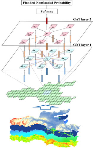
The GAT specializes in graph-structured data and has shown its efficacy in extracting the spatial dependency of the graph (Zhang et al. Citation2019). In general, the graph-structured data presents a non-linear structure consisting of nodes connected with edges, and the corresponding data values are attached to the nodes and edges. A GAT model consists of several layers. For each layer, the input is a set of node features. The model structure allows every node to attend to itself and its neighbors based on a shared attention mechanism, which means considering the attended nodes’ features to calculate its new features as the layer’s output. There can be more than one group of attentions for each node, and each group is called a head. After feature transformation through two GAT layers or more, the node information can be transmitted one by one across the whole graph. Finally, the feature output of the last GAT layer is transformed into the final output of the model for specifying the probability of each node belonging to any class.
Specific to the goal of mapping flood susceptibility, the nodes in the graph are individual units in the study area (shown in ). Node features represent the physical conditions of each unit and are extracted from the raw flood conditioning factors. The edges that link the nodes in the graph are constructed based on the relative spatial positions of different units.
Figure 1. The model structure of a GAT with two graph convolutional layers (four head attention mechanisms for the first layer and one for the second). the study area is firstly decomposed into a graph composed of nodes based on the relative spatial positions, and each node represents an individual unit in the study area. The features of each unit will go through multiple GAT layers for information aggregation. The output of the final layer is transformed into the results of each unit’s flooded and nonflooded probability using softmax function.
2.2. Model algorithm
The GAT comprises multiple graph convolutional layers to extract the spatial distribution of the input features and realize the node feature transformation. Through each layer, the feature of each node is updated by aggregating feature information through edges from its attended nodes. The features of all nodes change together when processed through the layer. After being processed with no less than two graph convolutional layers, a node can aggregate the information across the whole graph.
The algorithm of each graph convolutional layer is specifically indicated in . As the key of the GAT, the attention mechanism is used to learn the attention weights between pairs of connected nodes for effective feature extraction. The attention mechanism is parametrized with a specific matrix and a vector to calculate the assigned attention of one node to each direction. The learned attention weight can explicitly quantify how a node extracts information from its neighborhood in the form of probability. The graph convolutional function of the GAT can be described as:
(1)
(1)
(2)
(2)
(3)
(3)
(4)
(4)
where
is the original features of a single node in layer
and
denotes the node’s updated features, which then serves as the node’s input feature for layer
+1;
represents the neighborhood of the node i.
and
are the only two parameters required to be updated through iterations during the model training process; while the other variables are all intermediate variables.
Figure 2. The algorithm of one graph convolutional layer (modified from Veličković et al. (Citation2018)). The left indicates the process of calculating the attention weight that a node assigns to its neighbor (EquationEquations (1)–(3)). The right illustrates how the model transforms the original feature of the node to the updated feature based on the calculated attention weight (EquationEquation (4)(4)
(4) ).
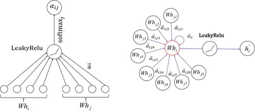
First, EquationEquation (1)(1)
(1) operates a linear transformation with a weight matrix,
on the lth layer node feature,
Subsequently, the features of the two nodes transformed in EquationEquation (1)
(1)
(1) ,
and
are concatenated, and the leaky rectified linear unit (LeakyRelu) function (Goodfellow et al. Citation2016), a commonly used activation function to help the network learn complex patterns in the data, is applied to the dot product of the concatenated transformed features and weight vector,
EquationEquation (3)
(3)
(3) then computes a pairwise normalized attention score between two neighbors. Finally, EquationEquation (4)
(4)
(4) obtains the updated node feature by weighted summation of the node and its neighbors’ transformed features according to the calculated attention scores and transforming the sum with the LeakyRelu activation function. Specifically, the LeakyRelu function used in EquationEquations (2)
(2)
(2) and Equation(4)
(4)
(4) is as follows, where α (>0) need to be artificially set up:
(5)
(5)
Specific to the last graph convolutional layer, the output node feature continues to be processed with the softmax function to specify the class a node belongs to in terms of probability (shown in ). The softmax function is a normalization function that enables each component of the output vector of a network to fall in the interval (0, 1), and the sum of all the transformed components is 1. The softmax function has also been used in EquationEquation (3)(3)
(3) for calculating the normalized attention scores, and its general mathematical presentation is as follows:
(6)
(6)
where
is the ith component of the vector and L is the total number of classes.
The attention mechanism can be extended to multi-head attentions to stabilize the learning process of attention weight assignment (Vaswani et al. Citation2017). The mechanism in all heads follows the same graph convolutional computation as illustrated in EquationEquation (1)(1)
(1) to Equation(4)
(4)
(4) . The aggregated features from each head are concatenated (for the non-last layer) or averaged (for the last layer) to obtain the new node features. According to the principle of the GAT, parallel operations across paired nodes are available, which will significantly improve the computational efficiency.
When applied to the urban pluvial flood, the GAT can establish the relationships between flood conditioning factors and the corresponding propensity of each unit to flood and finally realizes the flood susceptibility mapping in the whole study area. A series of flood conditioning factors go through no less than two graph convolutional layers for spatial feature extraction in each layer and feature transformation across layers. For an individual unit, the physical conditions of all the units are considered for the establishment of the relationship, which realizes the sufficient exploitation of the spatial information for flood susceptibility mapping. Finally, the probability of each unit belonging to either flooded or nonflooded class is output.
2.3. Modelling steps
Applying GAT to flood susceptibility analysis involves four major steps: (1) graph construction; (2) data preparation; (3) model training and (4) model evaluation. They are described as follows.
2.3.1. Graph construction
Flood conditioning factor data are generally in grid format. To match up with the data, applying GAT in flood susceptibility mapping can use regular units of the same size for graph construction. Each unit is assigned a series of climatic, topographical, land use and drainage features. The conditioning factors of all units (N is the number of units, F represents the dimensions of features) are standardized and taken by the GAT as one input. A certain proportion of the units are labeled as flooded or nonflooded samples for training models.
Simultaneously, the adjacency matrix derived from the relative spatial positions of units is converted into a sparse matrix and entered into the GAT to represent the graph structure. If two units share common corners or edges, they are considered adjacent to each other, and the corresponding value in the adjacency matrix is set to 1; otherwise, it is set to 0. In addition, the self-to-self elements of the adjacency matrix are all set to 1 to represent that each unit can also assign attention weight to itself besides its neighbors. Specifically, units not located on the boundary of the study area, which are the majority, all have eight spatially adjacent units.
2.3.2. Data preparation
Firstly, flood inventory containing historic flood locations will be collected. The recorded flood locations are then used for labeling the units as flooded; the same number of units are selected for nonflooded areas by choosing sites located on high elevation, covering low built-up areas or having strong drainage capacity where flooding is rare, referring to previous studies (Chapi et al. Citation2017; Rahmati et al. Citation2020).
Collecting flood conditioning factors are another task in data preparation. The performance of previous machine learning models for flood susceptibility mapping highly depends on the input flood conditioning factors (Jato-Espino et al. Citation2019). Specific to the urban pluvial flood, the susceptibility is generally influenced by four categories of conditioning factors: climatic, topographic, land use and drainage factors. However, the specific selection of which factor in these four categories is influenced by the sample size and distribution pattern of a region. Commonly-used factors include precipitation, landform (elevation, slope, curvature, aspect, etc.), land use zoning, drainage density and proximity to drainage (Tehrany et al. Citation2014).
The attention mechanism of the GAT determines that an individual unit’s feature can be transferred through edges and aggregated with other units’ features across the entire graph. It is expected that the GAT can automatically extract the spatial information from neighbors and learn the complex relationships among the units. Tedious feature-engineering for input construction and selection, thus, can potentially be avoided. Only a limited number of indispensable basic factors are required by the GAT. Therefore, here we suggested rainfall, elevation, normalized built-up index and drainage density as the only four flood conditioning factors. Each of them can represent one of the four different feature categories alone. Other factors calculated based on the above four basic factors of an individual unit and its neighborhood, such as slope, curvature and distance to drainage, are not necessary.
2.3.3. Model training
K-fold cross-validation should be used to split the training and test datasets. Through the cross-validation, the impact of different sample splits on model performance can be weakened. The flooded and nonflooded samples are stratified sampled to keep the rate of flooded and nonflooded samples invariant in each fold. Each graph convolutional layer’s model parameters, including weight matrix, and weight vector,
are optimized based on the training datasets and the test datasets are used for evaluation. When mapping flood susceptibility, all the labeled data should be used for training.
2.3.4. Model evaluation
The model performance can be evaluated using four indicators, including accuracy (ACC), precision (P), recall (R) and F-score (F):
(7)
(7)
(8)
(8)
(9)
(9)
(10)
(10)
where TP is the true positive rate representing the proportion of samples that are actually positive and judged as positive, while TN is the true negative rate representing the proportion of samples that are actually positive but are judged as negative. Similarly, FP and FN denote the false positive rate and false negative rate, respectively. Here, the positive and negative samples are samples labeled as flooded and nonflooded when evaluating model performance on identifying flooded units, while as nonflooded and flooded when identifying nonflooded units. The threshold of susceptibility for defining the flooded or nonflooded class is typically defaulted as 0.5.
The receiver operating characteristic (ROC) curve and areas under the curve (AUC) are used for judging the model’s discrimination ability (Costache and Tien Bui Citation2020). The ROC curve is depicted by the true positive (TP) rate on the Y-axis and the false positive (FP) rate on the X-axis. The AUC value is equivalent to the probability that a randomly chosen positive example is ranked higher than a randomly chosen negative example. The AUC value ranges from 0.5 to 1, and a higher AUC value indicates a better classification performance.
Furthermore, Kappa is used to evaluate the degree of agreement between observed data and model predictions, considering the potential for chance agreement. Kappa is calculated as follows:
(11)
(11)
Here, observed agreement () and the hypothetical probability of chance agreement (
) are calculated by comparing observations to model predictions. Kappa can vary between −1 (a Kappa value less than 0 indicates chance agreement) and 1 (perfect agreement).
3. Application of the GAT model
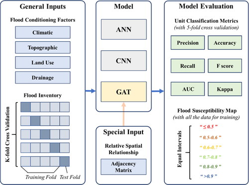
In this study, to assess the applicability of the GAT in pluvial flood susceptibility mapping in the context of data scarcity, a case study was carried out in the metropolitan area of Dalian, China. shows the overview of the data flow and workflow for the case study. The GAT was compared with another two state-of-the-art machine learning models for flood susceptibility mapping, ANN and CNN. The ANN was a simply-structured model and cannot take spatial information into consideration, while the CNN partially utilized spatial information within a limited range. All the three models were trained and tested on the same dataset given the same flood conditioning factors as inputs.
Figure 3. The overview of data flow and workflow for GAT, ANN and CNN. All the models were given four flood conditioning factors as inputs representing climatic, topographic, land use and drainage conditions. For GAT, there was another unique input, the adjacency matrix, which was derived based on the relative spatial positions of units in the study area. Five-fold cross-validation was implemented for evaluating the classification abilities of the three models, while the flood susceptibility maps for comparison were output by training models with all the data in the flood inventory. Finally, the flood susceptibility was classified into six levels for visualization.
3.1. Case information for graph construction
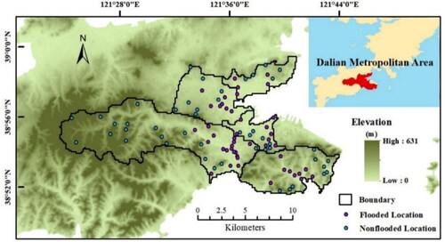
Dalian lies in the south of Liaodong Peninsula, China, located between 38°43′ and 40°12′ N and 120°58′ and 128°31′ E, covering an area of 187 sq. km. The annual average precipitation in Dalian is approximately 682 mm and approximately 60%–70% of the precipitation occurs from June to August. In recent years, the impact of flooding has kept rising due to the increased surface runoff, flow velocity and flow peak driven by continuous urbanization. Generally, the ponding depth in the study area is within the scope of 0.2 m–0.5 m.
As shown in , the Dalian metropolitan area was transformed into a graph comprised of 8312 units (150 × 150 m), and the relative spatial relationship between units was documented in the form of an 8312 × 8312 adjacency matrix composed of 0 and 1 entries. 150 m × 150m unit size met the objective of identifying flood-prone areas in large urban settings and was compatible with the community-level scale for collecting flooded sample. Moreover, this configuration allowed the generalized graph to be of an appropriate magnitude, ensuring computational efficiency of the GAT.
Figure 4. Study area and the distribution of flood inventory. The Dalian metropolitan area consists of five drainage divisions. There are 47 flooded records and 47 nonflooded records collected for the training.
Based on the information propagation mechanism of GAT, integrating global information theoretically requires only two layers of graph networks. Increasing the number of layers excessively will turn to weaken the model’s generalization capability (Wu et al. Citation2021). Therefore, here, a two-layer GAT model was constructed. The first layer consisted of four parallel attention heads to be compatible with the dimension of the input flood conditioning factors for efficient attention as suggested by previous studies (Bolya et al. Citation2022). Each head transformed the four-dimension input vector into a three-dimension vector. Then the four three-dimensional vectors were concatenated. The second layer was used for classification and only contained one single attention head that resulted in two-dimension features (which corresponded to the probabilities of two classes: flooded or nonflooded) from the outputs of the first layer. The parameter of the LeakyRelu function in each layer, α, was set to 0.2.
3.2. Case information for data preparation
3.2.1. Flood inventory
The flood inventory used in this study was provided by the Dalian Urban Construction Bureau. It includes 47 flooded samples frequently inundated by pluvial floods in various rainfall events from 2004 to 2014. The 47 flooded samples are the most flood susceptible locations in the study area and were regarded as flooded samples for model training. Meanwhile, an equal number of nonflooded samples were chosen based on the rules mentioned in previous studies (Zhao et al. Citation2019): 47 locations in either high elevations and high drainage capacity areas or low built-up areas were chosen as nonflooded samples. The locations of all the 94 flooded and nonflooded samples are shown in . The units (150 × 150 m) containing flooded or nonflooded samples were labeled as flooded or nonflooded units. All samples were located in different individual 150 × 150 m units.
3.2.2. Conditioning factors
Based on previous study (Fu et al. Citation2022) and data availability in the study area, four conditioning factors, average of annual maximum daily precipitation (AP), average elevation value (EV), pipe diameter weighted drainage density (WDD) and normalized differential built-up index (NDBI), were chosen to quantify the climate, topography, drainage and land use, respectively (shown as ). Their source, period, and spatial resolution of raw data are given in . All the factors went through standardization and were spatially averaged within the unit.
Figure 5. Four conditioning factors used in this study: (a) average of annual maximum daily precipitation (AP); (b) average elevation value (EV); (c) pipe diameter weighted drainage density (WDD); (d) normalized differential built-up index (NDBI).
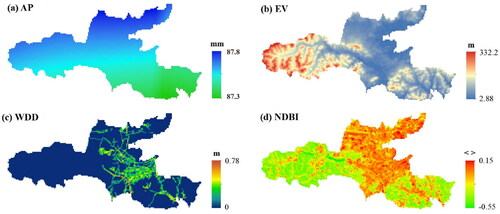
Table 1. Data source for the conditioning factor.
3.2.2.1. Climatic factor
Precipitation is one of the driving factors of urban pluvial flooding. In this study, AP between 2004 and 2014 (the same as the period of flood inventory) was introduced to represent the precipitation characteristics of the study area. Since the average precipitation (AP) was a long-term rainfall statistic used at the planning level, it demonstrated relatively minor spatial variation (0.5 mm) among different units within the study area.
3.2.2.2. Topographic factor
The average EV of each unit was adopted to represent the topographic characteristics. The explicit attention mechanism of the GAT was expected to induce the same information of the slope, curvature, aspect and other topographic factors from the graph instead of directly using them as inputs.
3.2.2.3. Drainage factor
Drainage capacity has a profound effect on the magnitude of urban flooding. To consider both the length and the diameter of the drainage pipe, here, WDD was used to characterize the drainage capacity. The raw data of the drainage networks were in a shapefile format, so they were first rasterized into a 30 m resolution Tiff image, and the value assigned to each grid was given by the diameter of the pipe crossing the grid. WDD was calculated as follow:
(12)
(12)
where A is the total number of grids in the unit, and in this study, A was set to 25 constantly (there are 25 grids of 30 × 30 m in a unit of 150 × 150 m). n is the number of grids overlain by pipes and denotes the diameter of the pipe crossing grid
3.2.2.4. Land use factor
The occurrence of urban flooding also closely correlates to the spatial pattern of land use. This study used the NDBI (Guo et al. Citation2015) calculated by EquationEquation (13)(13)
(13) from Landsat 8 remote sensing images to represent the impervious rate of the area so that the land use factor was described.
(13)
(13)
where MIR and NIR represent the middle infrared band and near infrared band of the Landsat images, respectively. The selected raw remote sensing image has already gone through atmospheric correction and was not contaminated by cloud cover.
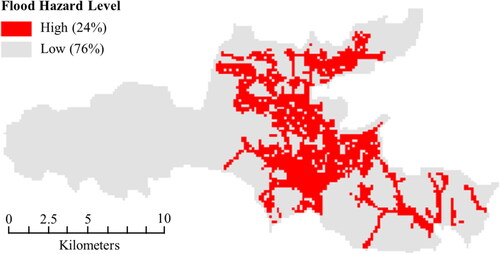
3.2.3. Validation data
To evaluate the rationality of the spatial pattern of flood susceptibility maps produced by different machine learning models, this study adopted the flood hazard map reported in the official stormwater management planning report from the Dalian Planning Department as validation data. The map was generated using MIKE Flood model given a 24-h, 100-year design rainfall event. As shown in , a unit (150 m × 150m) containing sites with a maximum water depth exceeding 0.2 m was classified as having high flood hazard level. High/Low Clustering analyses were performed on the map, as well as on the flood susceptibility maps produced by the three machine learning models, enabling a comparison of the degree of clustering for high flood hazard or susceptibility levels using the Getis-Ord General G statistic (Getis and Ord Citation1992).
Figure 6. Flood hazard map generated by MIKE flood model. The flood hazard level in each unit represents whether flooded sites (with a maximum water depth >0.2 m) exist within it or not. The percentage of each level in the study area is shown in the legend.
3.3. Case information for model training
We adopted fivefold cross-validation for model training and evaluation. An equal number of flooded and nonflooded samples were selected for each fold through stratified sampling. A negative log-likelihood function (Miranda Citation2017) was adopted as the loss function, and the learnable matrix and vector were optimized with the adaptive moment estimation optimizer (Kingma and Ba Citation2015). When training GAT, ANN and CNN, the number of training epochs was set as 200. For the first 100 epochs, the learning rate was configured as 0.01, and from the 101st epoch to the 200th epoch, the learning rate descended to 0.001 to finetune the model parameters. The model achieving the least loss value in the 200 training epochs was selected as the optimal model for subsequent evaluation and analysis. L2 regularization (Cortes et al. Citation2004) was used to avoid overfitting in training datasets.
3.4. Case information for model evaluation
We compared the GAT with an ANN model and a CNN model to evaluate the GAT’s performance on flooded-nonflooded sample classification and flood susceptibility mapping. The ANN model was a non-biased ANN model degenerated from the GAT with no pairs of units connected. The hyperparameter settings of the ANN model were the same as those of the GAT, with the exception that it could not incorporate neighborhood feature information into the feature transformation process of an individual unit, as GAT did. The construction of the CNN model here referred to the previous study (Wang et al. Citation2020). The CNN model comprised one convolutional layer, one pooling layer and one fully-connected layer. The input of CNN was set as 5 × 5-unit images of flood conditioning factors to estimate the flood susceptibility of the site located at the center of the images. The CNN model could utilize the neighborhood information during calculation but was limited to 5 × 5 units.
All the models were trained on the same dataset using the same training strategy. Five-fold cross-validation (80% training set; 20% test set) was adopted to obtain a relatively robust result not influenced by sample selection. As for flood susceptibility mapping, all the samples were used for training so that the flood inventory was fully exploited.
4. Results
4.1. Flooded-nonflooded sample classification performance
Model performance on flooded-nonflooded sample classification was evaluated with the average and standard mean square deviation of all the evaluation indicators of the five experiments in cross validation (). The performance of the GAT on both training and test datasets was superior to that of the ANN; the CNN performed better than the GAT on training datasets, while the GAT surpassed the CNN in terms of most indicators on test datasets. It indicated that the GAT was not subjected to the overfitting phenomenon as the CNN.
Table 2. Results of the GAT, ANN and CNN on the classification task with the average and standard mean square deviation of the five evaluation indicators of the five experiments in cross validation.
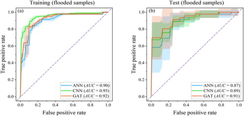
Another indicator, AUC, was then used for further comparing the GAT with the ANN and CNN in terms of the model’s ability on the classification task. The average and mean square deviation of ROC curves for five folds in cross validation and corresponding AUC values are shown in . On the test dataset, the GAT outperformed both the ANN and CNN for flooded samples with a higher AUC value (0.91). The higher sensitivity of the GAT to the susceptibility threshold indicated the higher discrimination capacity of the graph-based model structure. Compared to the other two models, the GAT was more generalizable.
Figure 7. Performance of the GAT, ANN and CNN in terms of the ROC curve. The color bars represent the standard mean square deviation of the true positive rate for the five cross-validation experiments, varying with the false positive rate.
4.2. Flood susceptibility map
The flood susceptibility maps produced by the GAT, ANN and CNN are shown in , respectively. The computed flood susceptibility values were categorized into six classes by applying fixed threshold values of 0.5, 0.6, 0.7, 0.8 and 0.9, for more straightforward visualization.
Figure 8. Comparisons of the flood susceptibility maps obtained by the (a) GAT, (b) ANN and (c) CNN and (d) the percentage of areas at different flood susceptibility levels predicted by the three models.
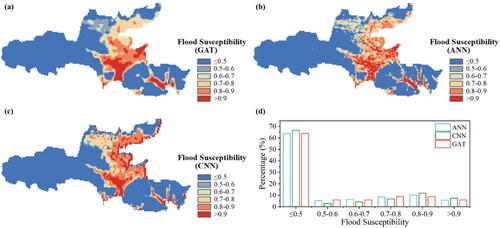
In terms of distribution pattern, the high flood susceptible areas appeared to be centralized in the flood susceptibility map produced by the GAT; in contrast, the flood susceptibility in the ANN output presented a more progressive distribution from low to high. The CNN was somewhere in between. As shown in , the region with a flood susceptibility exceeding 0.9, as identified by GAT (6.3%), was smaller than that identified by CNN (7.4%) but greater than that identified by ANN (5.8%). Additionally, the areas with flood susceptibility not exceeding 0.5 identified by ANN, CNN, and GAT were similar, accounting for 63.7%, 66.9% and 64.2% of the study area, respectively.
The degree of clustering for high flood susceptibility levels in different flood susceptibility maps was compared with that for high flood hazard in MIKE Flood simulations. Based on the High/Low clustering analysis, MIKE Flood presented a z-score of over 10, indicating a high level of clustering in areas with high flood hazard levels. Both GAT and CNN also exhibited patterns of high-level flood susceptibility clustering, with GAT achieving a z-score of 4.7, higher than that of CNN (3.9). In contrast, ANN achieved a z-score of −0.22, indicating a random distribution of high and low flood-susceptible areas. These results indicated that the flood susceptibility map generated by GAT exhibited a higher degree of consistency with the spatial clustering pattern presented in the simulation results of MIKE Flood, thus justifying it as the more rational model.
4.3. Verification of GAT’s informative feature extraction capability
To evaluate the GAT’s ability to extract informative features from basic flood conditioning factors, a correlation analysis was conducted between the model’s hidden features and a relevant physical variable. Specifically, the 16-dimensional features obtained from GAT’s first layer were utilized as inputs, while a high-order variable derived from elevation, slope, was employed as the target vector for training a linear regression model. The linear regression model’s fitting performance is equivalent to the correlation between the intermediate variable vector and slope, evaluated by the explanatory variance score () (Neter et al. Citation1996).
ranges from 0 to 1, a larger value of
typically means that the independent variables can better explain the variation in the dependent variable. For comparison, the initial four-dimensional flood conditioning factors as well as the 16-dimensional features of the first layer in the ANN and CNN were also adopted as inputs, respectively.
As shown in , although the ANN model did not consider neighborhood information, there was still a relatively strong correlation between the ANN’s intermediate variables and the slope (>0.5). Compared with the ANN, the updated feature vector obtained by GAT’s aggregating the features of one-hop neighbors had a better correlation with slope, especially in the flooded samples, increasing
by 0.11. CNN model could utilize the spatial information within a limited extent, but it achieved the lowest
among the three models. The low correlations between CNN’s intermediate variables and slope indicated that it did not perform cross-unit information transmission in a similar manner like GAT.
Table 3. The correlation () between the intermediate variables of different models and the slope for flooded and nonflooded samples.
The updated features of the GAT’s first layer undergo a single round of information propagation among units, while the slope represents the first-order derivative of elevation. Theoretically, these two elements are consistent in terms of the information they convey. The above result aligned with this consistency and indicated the GAT’s capability to automatically extract information related to high-order features for establishing a more generalizable mapping relationship. Therefore, the GAT could effectively map flood susceptibility using only basic flood conditioning factors. There was no need for additional input construction and selection, simplifying the modeling process.
5. Discussion
5.1. Effectiveness of GAT given limited inputs and samples for urban flood susceptibility mapping
GAT, trained on 94 samples, outperformed two other models named ANN and CNN in the metropolitan area of Dalian. It achieved an average accuracy of 0.85 on both the training and testing datasets during cross-validation. The inputs for GAT consisted of only four flood conditioning factors related to climate, terrain, drainage capacity and land use. These four input variables are all basic but indispensable factors in their respective categories. In comparison to a previous study conducted by Fu et al. (Citation2022), who used a similar number of flooded samples (50) to train an SVM model also in Dalian. However, the SVM’s accuracy (0.76) was lower than that of GAT, even though additional flood conditioning factors such as slope and topographic wetness index (TWI) derived from elevation were used. These results validate the effectiveness of GAT in urban flood susceptibility mapping based on only basic flood conditioning factors when using a limited number of samples.
The effectiveness of GAT can be attributed to its graph-based information propagation pattern, which imitates the hydrological responses among different units. The GAT takes the relative spatial positions as prior knowledge and its attention mechanism can be considered a resource allocation scheme to selectively consider adjacent units’ features for subsequent feature extraction (Niu et al. Citation2021). The correlation analysis between the model’s intermediate variables and slope further demonstrates the GAT’s automatic and effective extraction of high-order features. This capability enables model applications given limited basic flood conditioning factors. Such concise model construction is repetitive and can be directly applied to different areas, adopting a consistent input preparation procedure.
While GAT has demonstrated its superiority in classifying flooded and nonflooded samples, this came at the cost of longer computation times and higher computational expenses. As shown in , even though the three models have a similar number of model parameters, GAT required far more training time compared to the other two models. GAT involves parallel computations of a large number of nodes during training and prediction, resulting in substantial resource consumption, its resource requirements will continue to increase exponentially with the increase in the number of units.
Table 4. Training time and model parameter size for three models.
5.2. Spatial distribution characteristics of urban flood susceptibility
As described in Section 4.2, the identified relatively high flood susceptible areas by GAT were more centralized compared to CNN and ANN. ANN produced a map with a pattern more following the fluvial flood: from high-elevation regions to low-elevation regions within the flood-prone plains, the low flood susceptibility gradually transitioned to high susceptibility along the ridges in the terrain (Albertini et al. Citation2022; Zzaman et al. Citation2021). Referring to previous studies that applying machine learning model for urban flood susceptibility mapping, high flood susceptible areas are typically located in low-elevation regions where mainly high-density of buildings and roads as well as drainage networks (Li et al. Citation2023; Ouma and Omai Citation2023). The centralized distribution pattern presented by GAT more conformed to the previous conclusions. This was also verified by the flood hazard map generated by MIKE Flood model.
The clustering of high flood susceptible areas can primarily be attributed to the relatively coarse spatial resolution. Flood susceptibility mapping is commonly used to rapidly identify critical flood management areas in large-scale urban settings. To ensure efficiency and accommodate the limited number and quality of flood records (typically at community-level), a broader spatial scale is generally acceptable as long as it aligns with the necessary flood management requirements. Aggregating spatial data to coarser resolutions can introduce smoothing effects. Fine-scale heterogeneity and variability may be obscured or averaged out, leading to a loss of local variations and detailed features, thus a centralized pattern will present (Seleem et al. Citation2022).
Furthermore, the aggregation of high flood susceptible areas is also influenced by the type of samples used for model training. In this study, the collected flood events exclusively comprised pluvial floods caused by manhole overflow and local waterlogging, rather than other types of flood hazards such as flash or fluvial floods. Thus, there was a high concentration of flood susceptible areas within urbanized regions. If training samples belonging to other flood types are included, it might lead to biased spatial distributions of flood susceptibility, which characterize flood hazard from different perspectives.
5.3. Limitations and future works
Though the study area in this study is composed of only 8312 units (150 × 150 m) restricted by our existing computational resources, the GAT potentially applies to larger areas with different shapes. With the superiority in handling graph-structured data, the GAT can be extended flexibly. The state-of-the-art graph processing techniques such as subgraph clustering (Chiang et al. Citation2019; Gao et al. Citation2018) or random neighbor sampling (Hamilton et al. Citation2017) can further increase the magnitude of the graph that the GAT can efficiently process. The maximum number of nodes and edges that the GNN can handle has already reached the billion level (R. Ying et al. Citation2018), implying that it is possible to apply the GAT to a larger-scale catchment.
In addition, the influence of the spatial distribution of flooded and nonflooded samples on the prediction of flood susceptibility remains to be further addressed. In this study, a cross-validation approach was employed to minimize this influence. However, a standardized paradigm for selecting nonflooded samples has not yet been used. Future work could explore iterative optimization methods to automatically select a representative set of nonflooded samples within the study area, thereby avoiding potential biases introduced by manual selection (Tang et al. Citation2019). Additionally, it is also worth exploring positive-unlabeled learning algorithms that do not require labeled nonflooded samples (Li et al. Citation2022). Furthermore, new data sources such as crowdsourcing (Kong et al. Citation2022) and social media (Zeng et al. Citation2020), can provide more detailed training data to improve the GAT’s performance. Trained with not only the location information but also the flood magnitude, the GAT can derive more robust flood susceptibility results. In addition, the model’s potential for direct use in various cities, known as transferability (Seleem et al. Citation2023), remains to be explored.
The GAT also has the potential for flooding mechanism interpretation. The model’s learned attention weight correlates to the degree of hydrological response that one unit assigns to its adjacent units and itself, which will contribute to the interpretation of the flooding process and the analysis of the flood cause. The rationality of the automatically learned weight matrix and the interpretability of the GAT will be further validated by both hydrodynamic models and in-situ observations and be linked to specific physical variables using correlation diagnostic method such as probe (Lees et al. Citation2022).
6. Conclusion
Flood susceptibility mapping is the prerequisite for effective urban flood mitigation. Machine learning methods are increasingly applied, but the uncertain relationship between the limited data quantity and the necessary inputs limits the predictive performance and extensive application of models. This study introduced a semi-supervised graph-structured model, GAT, to deal with the limited number of flood inventory based on only basic flood conditioning factors. The model was assessed in the Dalian metropolitan area, China, and was compared with a non-biased ANN and a CNN model.
The GAT transformed the study area into a graph comprised of multiple nodes and links representing different units and their relatively spatial relationships and calculated the flood susceptibility in each unit. The GAT learned the mapping relationship between flood conditioning factors and flooded/nonflooded labels from both labeled and unlabeled units. The feature extraction by GAT imitated the hydrological responses among the spatial units. During the modeling process, an individual unit could extract valuable information from its neighborhood using only basic flood conditioning factors as inputs.
We concluded that, given 94 labeled samples, the GAT outperformed other models in flooded-nonflooded sample classification, and the spatial distribution of flood susceptibility presented by the GAT more conformed to reality. The GAT’s integration of spatial information by node also enables the simplicity of the input preparation. The GAT eliminates the need for an additional feature engineering procedure specific to the local environment while accurately mapping the flood susceptibility based on four indispensable factors characterizing climatic, terrain, drainage and land use conditions, respectively.
Therefore, GAT can adopt a concise paradigm for input preparation to address the data-scarcity challenge. It has the potential to become an effective tool in practical urban flood management. In the future, GAT can be applied to larger areas combined with higher-quality and finer-scale flood information. Furthermore, the capability of the GAT to interpret the flooding mechanism based on its attention mechanism is worth being evaluated in the subsequent work.
Author contribution
Z.W.: Conceptualization, Investigation, Methodology, Software, Writing—original draft; H.L.: Conceptualization, Writing—review & editing; C.Z.: Supervision, Funding acquisition.
Data availability Statement
The drainage network data and the flooded location information are provided by Dalian Municipal Bureau of Housing and Urban-Rural Development. China Meteorological Forcing Dataset can be downloaded from (http://data.cma.cn), ASTER GDEM (V1) product can be downloaded from (https://search.earthdata.nasa.gov/) and the Landsat TM/ETM product can be accessed through (https://www.usgs.gov/).
Disclosure statement
No potential conflict of interest was reported by the authors.
Additional information
Funding
References
- Abdelal Q, Al-Hmoud A. 2021. Low-cost, low-energy, wireless hydrological monitoring platform: design, deployment, and evaluation. J Sens. 2021:1–14doi: 10.1155/2021/8848955.
- Abedi R, Costache R, Shafizadeh-Moghadam H, Pham QB. 2022. Flash-flood susceptibility mapping based on XGBoost, random forest and boosted regression trees. Geocarto Int. 37(19):5479–5496doi: 10.1080/10106049.2021.1920636.
- Al-Areeq AM, Saleh RAA, Ghanim AAJ, Ghaleb M, Al‑Areeq NM, Al-Wajih E. 2023. Flood hazard assessment in yemen using a novel hybrid approach of grey wolf and Levenberg Marquardt optimizers. Geocarto Int. 38(1):1–20doi: 10.1080/10106049.2023.2243884.
- Albertini C, Miglino D, Iacobellis V, De Paola F, Manfreda S. 2022. Delineation of flood-prone areas in cliffed coastal regions through a procedure based on the geomorphic flood index. J Flood Risk Management. 15(1):e12766doi: 10.1111/jfr3.12766.
- Alwosheel A, van Cranenburgh S, Chorus CG. 2018. Is your dataset big enough? Sample size requirements when using artificial neural networks for discrete choice analysis. J Choice Model. 28:167–182doi: 10.1016/j.jocm.2018.07.002.
- Bentivoglio R, Isufi E, Jonkman SN, Taormina R. 2022. Deep learning methods for flood mapping: a review of existing applications and future research directions. Hydrol Earth Syst Sci. 26(16):4345–4378doi: 10.5194/hess-26-4345-2022.
- Berthelot D, Carlini N, Goodfellow IJ, Papernot N, Oliver A, Raffel C. 2019. MixMatch: A Holistic Approach to Semi-Supervised Learning. CoRR. 454: 5049–5059. http://arxiv.org/abs/1905.02249.
- Boller D, Moy de Vitry M, D. Wegner J, Leitão JP. 2019. Automated localization of urban drainage infrastructure from public-access street-level images. Urban Water J. 16(7):480–493doi: 10.1080/1573062X.2019.1687743.
- Bolya D, Fu C-Y, Dai X, Zhang P, Hoffman J. 2022. Hydra attention: efficient attention with many heads. arXivdoi: 10.48550/ARXIV.2209.07484.
- Butcher B, Smith BJ. 2020. Feature engineering and selection: a practical approach for predictive models. The American Statistician. 74(3):308–309doi: 10.1080/00031305.2020.1790217.
- Chapi K, Singh VP, Shirzadi A, Shahabi H, Bui DT, Pham BT, Khosravi K. 2017. A novel hybrid artificial intelligence approach for flood susceptibility assessment. Environ Modell Software. 95:229–245doi: 10.1016/j.envsoft.2017.06.012.
- Chiang WL, Li Y, Liu X, Bengio S, Si S, Hsieh CJ. 2019. Cluster-GCN: an efficient algorithm for training deep and large graph convolutional networks. Proceedings of the ACM SIGKDD International Conference on Knowledge Discovery and Data Mining, 257–266doi: 10.1145/3292500.3330925.
- Cortes C, Research G, York N. 2004. L 2 regularization for learning kernels. Twenty-Fifth Conference on Uncertainty in Artificial Intelligence, 109–116.
- Costache R, Tien Bui D. 2020. Identification of areas prone to flash-flood phenomena using multiple-criteria decision-making, bivariate statistics, machine learning and their ensembles. Sci Total Environ. 712:136492doi: 10.1016/j.scitotenv.2019.136492.
- Daksiya V, Mandapaka PV, Lo EYM. 2021. Effect of climate change and urbanisation on flood protection decision-making. J Flood Risk Manag. 14(1):e12681doi: 10.1111/jfr3.12681.
- Dottori F, Martina MLV, Figueiredo R. 2018. A methodology for flood susceptibility and vulnerability analysis in complex flood scenarios. J Flood Risk Manag. 11(S2):S632–S645doi: 10.1111/jfr3.12234.
- Du S, Cheng X, Huang Q, Chen R, Ward P, Aerts JCJH. 2019. Brief communication: rethinking the 1998 China floods to prepare for a nonstationary future. Nat Hazards Earth Syst Sci. 19(3):715–719doi: 10.5194/nhess-19-715-2019.
- Falah F, Rahmati O, Rostami M, Ahmadisharaf E, Daliakopoulos IN, Pourghasemi HR, Pourghasemi HR, Gokceoglu C. 2019. 14—Artificial Neural Networks for Flood Susceptibility Mapping in Data-Scarce Urban Areas. In Spatial Modeling in GIS and R for Earth and Environmental Sciences, p. 323–336. Amsterdam, Netherlands: Elsevier. doi: 10.1016/B978-0-12-815226-3.00014-4.
- Fu S, Lyu H, Wang Z, Hao X, Zhang C. 2022. Extracting historical flood locations from news media data by the named entity recognition (NER) model to assess urban flood susceptibility. J Hydrol. 612(PC):128312doi: 10.1016/j.jhydrol.2022.128312.
- Gao H, Wang Z, Ji S. 2018. Large-scale learnable graph convolutional networks. Proceedings of the ACM SIGKDD International Conference on Knowledge Discovery and Data Mining, 1416–1424doi: 10.1145/3219819.3219947.
- Getis A, Ord JK. 1992. The analysis of spatial association by use of distance statistics. Geog Anal. 24(3):189–206doi: 10.1111/j.1538-4632.1992.tb00261.x.
- Giovannettone J, Copenhaver T, Burns M, Choquette S. 2018. A statistical approach to mapping flood susceptibility in the lower connecticut River Valley region. Water Resour Res. 54(10):7603–7618doi: 10.1029/2018WR023018.
- Gnecco G, Morisi R, Roth G, Sanguineti M, Taramasso AC. 2017. Supervised and semi-supervised classifiers for the detection of flood-prone areas. Soft Comput. 21(13):3673–3685doi: 10.1007/s00500-015-1983-z.
- Goodfellow I, Bengio Y, Courville A. 2016. Deep learning. Cambridge, MA, USA: MIT press.
- Guo G, Wu Z, Xiao R, Chen Y, Liu X, Zhang X. 2015. Impacts of urban biophysical composition on land surface temperature in urban heat island clusters. Landscape Urban Plann. 135:1–10doi: 10.1016/j.landurbplan.2014.11.007.
- Hamilton WL, Ying R, Leskovec J. 2017. Inductive representation learning on large graphs. Advances in Neural Information Processing Systems, 2017-Decem (Nips), 1025–1035.
- Ilia I, Tsangaratos P, Tzampoglou P, Chen W, Hong H. 2022. Flash flood susceptibility mapping using stacking ensemble machine learning models. Geocarto International. 37(27):15010–15036doi: 10.1080/10106049.2022.2093990.
- Jacinto R, Grosso N, Reis E, Dias L, Santos FD, Garrett P. 2015. Continental Portuguese territory flood susceptibility index—contribution to a vulnerability index. Nat Hazards Earth Syst Sci. 15(8):1907–1919doi: 10.5194/nhess-15-1907-2015.
- Jahangir MH, Mousavi Reineh SM, Abolghasemi M. 2019. Spatial predication of flood zonation mapping in Kan River Basin, Iran, using artificial neural network algorithm. Weather Clim Extremes. 25(July):100215doi: 10.1016/j.wace.2019.100215.
- Jato-Espino D, Lobo A, Ascorbe-Salcedo A. 2019. Urban flood risk mapping using an optimised additive weighting methodology based on open data. J Flood Risk Manag. 12(S1):e12533doi: 10.1111/jfr3.12533.
- Kingma DP, Ba JL. 2015. Adam: a method for stochastic optimization. 3rd International Conference on Learning Representations, ICLR 2015—Conference Track Proceedings, p. 1–15.
- Kohansarbaz A, Kohansarbaz A, Shabanlou S, Yosefvand F, Rajabi A. 2022. Modelling flood susceptibility in northern Iran: application of five well-known machine-learning models. Irrig Drain. 71(5):1332–1350doi: 10.1002/ird.2745.
- Kong X, Yang J, Qiu J, Zhang Q, Chen X, Wang M, Jiang S. 2022. Post-event flood mapping for road networks using taxi GPS data. J Flood Risk Manag. 15(2):e12799doi: 10.1111/jfr3.12799.
- Leandro J, Schumann A, Pfister A. 2016. A step towards considering the spatial heterogeneity of urban key features in urban hydrology flood modelling. J Hydrol. 535:356–365doi: 10.1016/j.jhydrol.2016.01.060.
- Lees T, Reece S, Kratzert F, Klotz D, Gauch M, De Bruijn J, Kumar Sahu R, Greve P, Slater L, Dadson SJ. 2022. Hydrological concept formation inside long short-term memory (LSTM) networks. Hydrol Earth Syst Sci. 26(12):3079–3101doi: 10.5194/hess-26-3079-2022.
- Li P, Yu Y, Huang D, Wang Z, Sharma A. 2023. Regional heatwave prediction using graph neural network and weather station data. Geophys Res Lett. 50:e2023GL103405. doi: 10.1029/2023GL103405.
- Li W, Liu Y, Liu Z, Gao Z, Huang H, Huang W. 2022. A positive-unlabeled learning algorithm for urban flood susceptibility modeling. Land. 11(11):1971doi: 10.3390/land11111971.
- Li Y, Osei FB, Hu T, Stein A. 2023. Urban flood susceptibility mapping based on social media data in Chengdu city, China. Sustain Cities Soc. 88:104307doi: 10.1016/j.scs.2022.104307.
- Masoumi Z. 2022. Flood susceptibility assessment for ungauged sites in urban areas using spatial modeling. J Flood Risk Manag. 15(1):e12767doi: 10.1111/jfr3.12767.
- Miranda LJ. 2017. Understanding softmax and the negative log-likelihood. Ljvmiranda921.Github.Io
- Neter J, Kutner MH, Nachtsheim CJ, Wasserman W, et al. 1996. Applied linear statistical models, 318. Vol. 4. Chicago: Irwin.
- Niu Z, Zhong G, Yu H. 2021. A review on the attention mechanism of deep learning. Neurocomputing. 452:48–62doi: 10.1016/j.neucom.2021.03.091.
- Nsangou D, Kpoumié A, Mfonka Z, Bateni SM, Ngouh AN, Ndam Ngoupayou JR. 2022. The Mfoundi watershed at Yaoundé in the humid tropical zone of Cameroon: a case study of urban flood susceptibility mapping. Earth Syst Environ. 6(1):99–120doi: 10.1007/s41748-021-00276-9.
- Ouma YO, Omai L. 2023. Flood susceptibility mapping using image-based 2D-CNN deep learning: overview and case study application using multiparametric spatial data in data-scarce urban environments. Int J Intell Syst. 2023:1–23doi: 10.1155/2023/5672401.
- Prasad P, Loveson VJ, Das B, Kotha M. 2022. Novel ensemble machine learning models in flood susceptibility mapping. Geocarto Int. 37(16):4571–4593doi: 10.1080/10106049.2021.1892209.
- Rahmati O, Darabi H, Panahi M, Kalantari Z, Naghibi SA, Ferreira CSS, Kornejady A, Karimidastenaei Z, Mohammadi F, Stefanidis S, et al. 2020. Development of novel hybridized models for urban flood susceptibility mapping. Sci Rep. 10(1): 1–19. doi: 10.1038/s41598-020-69703-7.
- Ran J, Nedovic-Budic Z. 2016. Integrating spatial planning and flood risk management: a new conceptual framework for the spatially integrated policy infrastructure. Comput Environ Urban Syst. 57:68–79doi: 10.1016/j.compenvurbsys.2016.01.008.
- Saber M, Boulmaiz T, Guermoui M, Abdrabo KI, Kantoush SA, Sumi T, Boutaghane H, Nohara D, Mabrouk E. 2022. Examining LightGBM and CatBoost models for wadi flash flood susceptibility prediction. Geocarto International. 37(25):7462–7487doi: 10.1080/10106049.2021.1974959.
- Seleem O, Ayzel G, Bronstert A, Heistermann M. 2023. Transferability of data-driven models to predict urban pluvial flood water depth in Berlin, Germany. Nat Hazards Earth Syst Sci. 23(2):809–822doi: 10.5194/nhess-23-809-2023.
- Seleem O, Ayzel G, de Souza ACT, Bronstert A, Heistermann M. 2022. Towards urban flood susceptibility mapping using data-driven models in Berlin, Germany. Geomatics Nat Hazards Risk. 13(1):1640–1662doi: 10.1080/19475705.2022.2097131.
- Sun Y, Xie Z, Wang H, Huang X, Hu Q. 2022. Solar wind speed prediction via graph attention network. Space Weather. 20(7):e2022SW003128doi: 10.1029/2022SW003128.
- Tang X, Hong H, Shu Y, Tang H, Li J, Liu W. 2019. Urban waterlogging susceptibility assessment based on a PSO-SVM method using a novel repeatedly random sampling idea to select negative samples. J Hydrol. 576:583–595doi: 10.1016/j.jhydrol.2019.06.058.
- Tehrany MS, Lee MJ, Pradhan B, Jebur MN, Lee S. 2014. Flood susceptibility mapping using integrated bivariate and multivariate statistical models. Environ Earth Sci. 72(10):4001–4015doi: 10.1007/s12665-014-3289-3.
- Vaswani A, Shazeer N, Parmar N, Uszkoreit J, Jones L, Gomez AN, Kaiser Ł, Polosukhin I. 2017. Attention is all you need. Advances in Neural Information Processing Systems, 2017-Decem (Nips), 5999–6009.
- Veličković P, Casanova A, Liò P, Cucurull G, Romero A, Bengio Y. 2018. Graph attention networks. 6th International Conference on Learning Representations, ICLR 2018—Conference Track Proceedings, p. 1–12.
- Veličković P, Cucurull G, Casanova A, Romero A, Liò P, Bengio Y. 2017. Graph Attention Networks. arXivdoi: 10.48550/ARXIV.1710.10903.
- Vojtek M, Vojteková J. 2019. Flood susceptibility mapping on a national scale in Slovakia using the analytical hierarchy process. Water (Switzerland). 11(2):364doi: 10.3390/w11020364.
- Wang Y, Fang Z, Hong H, Peng L. 2020. Flood susceptibility mapping using convolutional neural network frameworks. J Hydrol. 582:124482doi: 10.1016/j.jhydrol.2019.124482.
- Wu Z, Pan S, Chen F, Long G, Zhang C, Yu PS. 2021. A comprehensive survey on graph neural networks. IEEE Trans Neural Netw Learn Syst. 32(1):4–24doi: 10.1109/TNNLS.2020.2978386.
- Ying R, He R, Chen K, Eksombatchai P, Hamilton WL, Leskovec J. 2018. Graph convolutional neural networks for web-scale recommender systems. Proceedings of the ACM SIGKDD International Conference on Knowledge Discovery and Data Mining, 974–983doi: 10.1145/3219819.3219890.
- Ying X. 2019. An overview of overfitting and its solutions. J Phys: conf Ser. 1168(2):22022doi: 10.1088/1742-6596/1168/2/022022.
- Young A, Bhattacharya B, Zevenbergen C. 2021. A rainfall threshold-based approach to early warnings in urban data-scarce regions: a case study of pluvial flooding in Alexandria, Egypt. J Flood Risk Management. 14(2):e12702doi: 10.1111/jfr3.12702.
- Zeng Z, Lan J, Hamidi AR, Zou S. 2020. Integrating internet media into urban flooding susceptibility assessment: a case study in China. Cities. 101(1037):102697doi: 10.1016/j.cities.2020.102697.
- Zhang C, Yu JJQ, Liu Y. 2019. Spatial-temporal graph attention networks: a deep learning approach for traffic forecasting. IEEE Access. 7:166246–166256doi: 10.1109/ACCESS.2019.2953888.
- Zhang W, Villarini G, Vecchi GA, Smith JA. 2018. Urbanization exacerbated the rainfall and flooding caused by hurricane Harvey in Houston. Nature. 563(7731):384–388doi: 10.1038/s41586-018-0676-z.
- Zhao G, Pang B, Xu Z, Cui L, Wang J, Zuo D, Peng D. 2021. Improving urban flood susceptibility mapping using transfer learning. J Hydrol. 602:126777doi: 10.1016/j.jhydrol.2021.126777.
- Zhao G, Pang B, Xu Z, Peng D, Xu L. 2019. Assessment of urban flood susceptibility using semi-supervised machine learning model. Sci Total Environ. 659:940–949doi: 10.1016/j.scitotenv.2018.12.217.
- Zzaman RU, Nowreen S, Billah M, Islam AS. 2021. Flood hazard mapping of Sangu River basin in Bangladesh using multi-criteria analysis of hydro-geomorphological factors. J Flood Risk Manag. 14(3):e12715doi: 10.1111/jfr3.12715.