Flood hazard mapping using GIS-based statistical model in vulnerable riparian regions of sub-tropical environment

Abstract

Floods are a recurrent natural calamity that presents substantial hazards to human lives and infrastructure. The study indicates that a significant proportion of the study area, specifically 27.05%, is classified as a moderate flood risk zone (FRZ), while 20.78% is designated as high or very high FRZ. The region’s low and very low FRZ are classified at 52.17%. The GIS-based AHP model demonstrated exceptional predictive precision, achieving a score of 0.749 (74.90%) as determined by the AUC-ROC, a widely used statistical evaluation tool. The current study has identified areas with high FRZ in the affected CD blocks, which are situated in low-lying flood plains, regions with gentle slopes, high drainage density, high TWI, low NDVI, high MNDWI, areas with high population density, intensive agricultural land. The findings of this research offer significant perspectives for decision-makers, city planners, and emergency management agencies in devising efficient measures to mitigate flood risks.

Keywords:

• Flood susceptibility
• flood vulnerability
• flood risk
• multi-collinearity

1. Introduction

Floods often occur when a river has more water than it can carry, and the capacity of its channels is exceeded. Floods are a prevalent form of natural disaster on a global scale, impacting a greater number of individuals than any other type of natural disaster. They constitute approximately one-third of all hazards worldwide (Das 2020; Hemmati et al. 2020; Slater et al. 2021; Petrucci 2022). Floods are regarded as a natural hazard due to their potential to harm both natural and anthropogenic environments. Recent years have seen a rise in the frequency of floods due to inappropriate land use planning, rapid population explosion, unorganized development process and unchecked urbanization (Das 2018; Hammami et al. 2019; Paul and Sarkar 2022). Over the last several decades, floods have become more destructive and potentially result in major economic losses and fatalities. Researchers from across the globe gave them serious consideration (Da Silva et al. 2020; Das 2020; Chiu et al. 2021). Flooding has caused an average of 6,500 deaths per year and $15 billion in damage annually over the past 20 years, according to the World Meteorological Organization (WMO). Information on the intensity, frequency, and different flood conditioning parameters that might produce rapid flooding during a flood event is needed for flood risk management (Das 2020; Mishra and Sinha 2020). All over the world, flood is a common hazardous phenomenon, frequently causing immeasurable human suffering and economic difficulties (Hemmati et al. 2020; Slater et al. 2021; Petrucci 2022), yet its severity varies across time and space. Global flooding patterns have risen over the last three decades, and this rise is entirely connected with the effects of drastic climate change, changes in land use patterns, and other anthropogenic intervention activities (Di Baldassarre et al. 2010, Kourgialas and Karatzas 2011; Chakraborty and Mukhopadhyay 2019).

India is known as the ‘land of monsoon’ (Subrahmanyam 1988; Chakraborty and Mukhopadhyay 2019; Das and Scaringi 2021), where the rainy season is praised for having a positive impact on the country’s agricultural output and economy (Paul and Mahmood 2016). However, for the 32 million people in the nation who experience an average yearly flood inundation, the monsoon also signifies a time of concern (Kale, 2004; Chakraborty and Mukhopadhyay 2019). Most of India’s historically destructive floods have been caused by the vagaries of the Indian summer monsoon’s unpredictable behaviour (Dhar and Nandargi 2003; Das 2020). These floods severely damaged crops, property, the economy, and human lives (Vishnu et al. 2019; Das 2020). According to the India Ministry of Ministry Home Affairs and Annual Report 2019–2020 (2020), India is highly susceptible to flooding, with more than 40 million hectares of land at risk. According to the Indian government, floods in 2021 affected over 17 million people across 15 states and caused over 1,000 deaths (India Ministry Home Affairs, Annual Report 2021-22, 2021). Some of the worst floods in India’s recent history include the 2018 Kerala floods, which killed over 400 people and caused over $4 billion in damage, and the 2019 Maharashtra floods, which killed over 50 people and displaced thousands (BBC, 2018). The Brahmaputra and Ganga rivers are particularly prone to flooding, with major floods occurring almost every year in these regions. (Down to Earth, 2020). When all the river floodplains in India are combined, around 48% of the country is reasonably protected from annual floods (Central Water Commission Annual Report 2009–10 2010). Historically, the floodplains have encouraged people to reside there because of their productivity and other long-term possibilities. Due to their geomorphic consequences, such as bank erosion, avulsion, and channel abandonment, annual floods are thought to be more important than rare major floods for regulating floodplains, specifically in the Ganga-Brahmaputra plains (Auerbach et al. 2015; Mehebub et al. 2015; Kumar, 2021; Pandey et al. 2022; Paul and Sarkar 2022). However, floods occasionally transform a natural occurrence into a natural catastrophe due to the loss of life and property. The Malda district has historically been devastated by floods due to the monsoon season’s torrential downpours and extremely high-water levels in almost all the district’s major rivers. Three different inundations that occurred between 1850 and 1870 caused severe misery in all areas of the district, particularly in the lowland areas around the rivers. Following 1870, the region was again affected by heavy floods in the years 1875, 1885, and 1906. Foods also had an impact in the years 1918, 1922, 1935, and 1948. In the following years, all districts were hit by severe flooding catastrophes in 1987, 1988, 1991, 1995, 1996, 1998, 1999, 2003, 2005, 2006, 2007, 2008, 2017, and 2019 (DDMPM 2020–2021). In various parts of the district, flowing flood water varied at a depth of 4 feet to 10 feet. These floods weren’t as much influenced by rain in the district as by overflowing rivers due to excessive rainfall in the upper catchment regions. Since many of the rivers and streams in the Malda district, including the Ganges, originate in the Himalayan Mountains, it is vulnerable to sudden and massive water inflows resulting from snow melting or intense rainfall in the region.

In recent times, evaluating flood risk zones (FRZ) has emerged as a complex and inventive undertaking for geologists, geomorphologists, hydrologists, hydrogeologists, and policymakers around the globe. The objective is to promote sustainable socio-economic progress (Souissi et al. 2019; Msabi and Makonyo 2021). United Nations Member States adopted the Sendai Framework for Disaster Risk Reduction (SFDRR) by the year 2015, aiming to reduce disaster risk and build resilience of communities and nations from 2015 to 2030. Its target is to reduce the number of affected people; between 2005 and 2014, approximately 1.7 billion people were affected by disasters, averaging 170 million per year. The SFDRR aims to reduce direct economic losses from disasters; between 2005 and 2014, these losses amounted to around $1.4 trillion globally. The framework’s objective is to enhance the count of nations that possess national and local strategies for reducing the risks associated with disasters. By 2021, 93 countries had reported progress in developing or updating such strategies. (Msabi and Makonyo 2021). The research area’s susceptibility and vulnerability have been mapped to create the Flood Risk Zone (FRZ). Therefore, while constructing the Flood Risk Zone (FRZ) assessment, it is crucial to model the Flood Susceptibility Zone (FSZ) and Flood Vulnerability Zone (FVZ). One of the most recent appropriate methodologies is multi-criteria decision making (MCDM), which is widely utilized to simulate such FSZ, FVZ, and FRZ (Ghosh and Kar 2018; Kafle and Shakya 2018; Edamo et al. 2022; Mitra et al. 2022; Paul and Sarkar 2022). It is critical to identify which choices are optimal. MCDM can rapidly produce and rank all possible options based purely on their efficacy (Mitra et al. 2022). In recent years, several scientists have used Remote Sensing (RS) and Geographic Information Systems (GIS) approaches to assess FRZ globally using MCDM methods with great accuracy.

Various researchers have developed hydrological models, including Hydraulic Engineering Center-River Analysis System (HEC-RAS) (Getahun and Gebre 2015; Tamiru and Dinka 2021; Hidayah, Halik, et al. 2022), Hydrologiska Byråns Vattenbalansavdelning model (HBV) (Grillakis et al. 2010), Soil Water Assessment Tool (SWAT) (Oeurng et al. 2011; Duan et al. 2019; Hidayah et al. 2021; Eingrüber and Korres 2022), Sub-Watershed Prioritization by Morphometric Analysis (SWPMA) (Hasanuzzaman et al. 2023), WetSpa (Bahremand et al. 2007) and HYDROTEL (Liu and De Smedt 2005; Azizi et al. 2018), and Hydrodynamic methods (Moore and Hutchinson 1990; Pei et al. 2010; Rousseau et al. 2015; Huang et al. 2019; Bhattacharjee et al. 2020; Liu et al. 2020; Elong et al. 2022; Wang et al. 2022; Jesna et al. 2023; Mondal et al. 2023; Olbert et al. 2023). Despite the capability of hydrological models to forecast and simulate flood hazards, they exhibit limitations such as the need for a substantial amount of data, lack of comprehensive large-scale data, and the time-consuming process of preparing and fine-tuning parameters (Rahmati et al. 2018; Sahraei et al. 2020; Noymanee and Theeramunkong 2019). Numerous research has been conducted to evaluate flood risk using MCDM methods (Wassenaar and Chen 2003; Jasrotia et al. 2007; Mondal et al. 2008; Chenini and Ben Mammou 2010; Jha et al. 2010; Elewa and Qaddah 2011; Ozdemir 2011; Adiat et al. 2012, Magesh et al. 2012; Agarwal and Garg 2015; Muralitharan and Palanivel 2015; Senanayake et al. 2016; Das et al. 2017; Keshavarz Ghorabaee et al. 2017), including the Multiple Criteria Analysis (Kafle and Shakya 2018; Mahmoud & Gan 2018; Sharma et al. 2018; Azareh et al. 2019; Bouamrane et al. 2020; Chen 2021; Costache et al. 2021; Pham et al. 2021), Analytical Hierarchy Process (AHP) (Ouma and Tateishi 2014; Kazakis et al. 2015; Gigović et al. 2017; Jenifer and Jha 2017; Mahmoud & Gan 2018; Radwan et al. 2018; Vijith and Dodge-Wan 2019; Das 2020; Mishra and Sinha 2020; Islam and Raja 2021; Tayyab et al. 2021; Hussain et al. 2023), Best-Worst Method (BWM) (Khiavi et al. 2023), Certainty Factor (CF) (Cao et al. 2020), Dempster-Shafer Evidential Belief Function (EBF) (Rahmati and Melesse 2016; Bui et al. 2019; Pradhan 2019; Shafapour Tehrany et al. 2019; Bhardwaj and Veerappan 2023); Evaluation Based on Distance from Average Solution (EDAS) (Ghorabaee et al. 2017; Mitra and Das 2022), Frequency Ratio (FR) (Sahoo et al. 2017; Samanta et al. 2018; Ullah and Zhang 2020; Hidayah et al. 2022; Hasanuzzaman et al. 2023), Fuzzy Analytical Hierarchy Process (FAHP) (Chang 1996; Hasanloo et al. 2019; Bouamrane et al. 2020; Costache et al. 2022), Fuzzy Logic (FL) (Malik et al. 2020; Akay 2021), Hydrological Modeling Approach (HMA) (Hidayah et al. 2021; Khiavi et al. 2023), Local Weighted Linear Combination (LWLC) (Solaimani et al. 2022), Logistic Regression (LR) (Özay and Orhan 2023), Ordered Weighted Average (OWA) (Solaimani et al. 2022), Preference Ranking Organization Method (Yougbaré 2019), Stochastic Multicriteria Acceptability Analysis (SMAA) (Xu et al. 2023), Technique for ranking Orders Preference by Similarity to the Ideal Solution (TOPSIS) (Sari 2021; Mitra and Das 2022; Solaimani et al. 2022), Vise Kriterijumska Optimizacijaik Ompromisno Resenje (VIKOR) (Sari 2021; Mitra and Das 2022; Xu et al. 2023), Weighted Linear Combination (WLC) (Solaimani et al. 2022), Weighted Multi-Criteria Analysis (WMCA) (Solaimani et al. 2022) and Weights of Evidence (WoE) (Tehrany et al. 2014; Sahoo et al. 2017; Costache et al. 2022; Hidayah et al. 2022). The techniques are based on assigned thematic layers based on Remote Sensing (RS) and Geographical Information System (GIS) framework. Certain machine learning algorithms are capable of effectively addressing complicated non-linear problems without the requirement for statistical assumptions (Karande and Chakraborty 2012; Pourghasemi et al. 2013; Mosavi et al. 2018; Chen et al. 2019; Costache 2019; Jahangir et al. 2019; Costache et al. 2020; Feby et al. 2020; Shahabi et al. 2020; Baig et al. 2021; Costache et al. 2021; Pham et al. 2021; Taromideh et al. 2022; Aldiansyah and Wardani 2023; Saikh and Mondal 2023) such as Analytic Network Process (ANP) (Khiavi et al. 2023), Artificial Neural Networks (ANN) (Costache et al. 2020; Islam et al. 2021), BAT Algorithms (BA) (Ahmadlou et al. 2019), Binomial Logistic Regression Model (BLR) (Chowdhuri et al. 2020), Biogeography-Based Optimization (BBO) (Moayedi et al. 2023), Boosted Regression Tree (BRT) (Lee et al. 2017; Kohansarbaz et al. 2022), Classification and Regression Trees (CART) (Taromideh et al. 2022), Convolutional Neural Network (CNN) (Ullah et al. 2022), Decision Trees (DTs) (Balamurugan et al. 2022), K-Nearest Neighbour (KNN) (Shahabi et al. 2020; Gauhar et al. 2021; Al-Aizari et al. 2022; Ullah et al. 2022), Logistic Regression (LR) (Tehrany et al. 2017; Ali et al. 2020; Pham et al. 2020; Ullah et al. 2022), Multi-Attributive Border Approximation area Comparison (MABAC) (Pamučar and Ćirović 2015), Multivariate Adaptive Regression Splines (MARS) (Taromideh et al. 2022; Aldiansyah and Wardani 2023), Multivariate Discriminant Analysis (MDA) (Taromideh et al. 2022; Aldiansyah and Wardani 2023), Multi-Layer Perceptron (MLP) (Hidayah et al. 2022), Naïve Bayes (NB) (Pham et al. 2020; Tang et al. 2020; Al-Aizari et al. 2022; Hasanuzzaman et al. 2022; Habibi et al. 2023), Neuro-Fuzzy Logic (Kulkarni and Shete 2014; Patel et al. 2014), Random Forest (RF) (Lee et al. 2017; Tang et al. 2020; Islam et al. 2021; Al-Aizari et al. 2022; Ghosh et al. 2022; Hidayah et al. 2022; Hasanuzzaman et al. 2023; Hussain et al. 2023), Reduced Error Pruning Trees (Saikh and Mondal 2023), Support Vector Machines (SVMs) (Tehrany et al. 2014; Shafapour Tehrany et al. 2019; Islam et al. 2021; Bera et al. 2022; Ghosh et al. 2022; Hussain et al. 2023), Shannon’s Entropy (Bera et al. 2022) and Extreme Gradient Boosting (XGBoost) (Al-Aizari et al. 2022; Aydin and Iban 2022; Ghosh et al. 2022).

Despite the availability of alternative approaches, the Analytical Hierarchy Process (AHP) (Saaty, 1977, 1980, 1987, 1990, Saaty 2006) remains the most widely used method for delineating FRZ due to its effectiveness and reliability. It aims to find optimal solutions. As flood risk can now be accurately quantified and mapped, there has been an increase in interest in applying the AHP to flood hazard assessment and management. The weights are assigned to thematic layers, and these layers are classified based on the available knowledge and the unique conditions of the site in several studies (Das 2018; Souissi et al. 2019; Abdelkarim et al. 2020; Cabrera and Lee 2020; Mishra and Sinha 2020; Das and Gupta 2021; Paul and Sarkar 2022; Hussain et al. 2023). The Bengal Delta region, a part of West Bengal, has a well-documented history of flooding. Currently, 42.55% to 55.80% of the State is at threat of flooding (Nath et al. 2008; Das et al. 2012; Das and Pal 2016; Mukherjee and Pal 2017; Mitra et al. 2022; Paul and Sarkar 2022). About 37,760 sq. km. of the total flood-prone area stretches 19 flood susceptible districts and 198 vulnerable blocks (Annual Flood Report 2019). The district’s terrain was created by the Ganga-Padma River system via the construction of a delta, with floods acting as the main source of the great bulk of fluvial deposits and the main carrier of sediments. In 1978, the worst affected area was about 30,607 sq. km, whereas in 2000, it was about 23,971 sq. km. About 11 States provide floodwater to the southern section of the district Malda, where the river Ganga runs, and this region is severely impacted by the excessive runoff flow produced by these vast regions. The river eventually flows into Bangladesh after passing through the Farakka Barrage. The Mahananda and Fulahar river systems drain into the western section of the Malda district, bringing in floodwater mainly from the neighbouring country of Nepal and the State of Bihar. After flowing directly south, Fulahar meets the Ganga upstream. At the same time, the Mahananda makes a U-turn to the southeast and divides the district Malda before draining into the Ganga-Padma downstream. The Mahananda and Fulahar systems catchment area is 19,342 sq. km. The runoff from localized high rainfall, discharge from upper catchment basins, and excessive runoff conditions in neighbouring countries are significant causes of flooding in North Bengal regions. During periods of high water levels in the Ganga, upstream and downstream of the Farakka Barrage, many rivers in the Uttar and Dakshin Dinajpur districts, such as the Mahananda, experience stagnation. This stagnation impedes the drainage of flood discharge in the affected areas.

The present research aims to achieve several objectives. The current investigation has three main objectives, namely: (a) to develop an all-inclusive framework for evaluating FS, vulnerability, and risk in the floodplain area of Malda District, West Bengal, India, by employing RS and GIS-based AHP methodology. It includes an assessment of multi-collinearity in the model, (b) conducting a sensitivity analysis of the AHP model to assess the impact of input parameters and their uncertainties on the outcomes of flood assessment, and (c) evaluating the dependability and precision of the GIS-based AHP model by comparing its results with historical flood events and ground-truth data. These objectives aim to ensure the suitability of the proposed model for flood risk management and decision-making in the region.

2. Materials and methods

2.1. Study area

The study area under consideration is the Malda district, situated within the latitudes 25°32′08″ North to 24°40′20″ North and longitudes 88°28′10″ East to 87°45′50″ East. The district is geographically situated adjacent to Murshidabad district towards the southern direction, while Uttar Dinajpur and Dakshin Dinajpur districts are located towards the northern direction (Figure 1). The eastern border of the district spans a length of 165.5 km and is shared with Bangladesh. Towards the western direction, the district shares its borders with Santhal Parganas of Jharkhand and Purnea of Bihar. The district covered an area of about 1,987 sq. miles (5146 sq. km.) in 1935 as per the survey and settlement operations report. During the partition of India, it had a coverage of approximately 2,004 sq. miles (5190 sq. km.), but after independence, the area has been reduced to about 1,441.6 sq. miles (3,733 sq. km.). Most of the low-lying alluvial plains in the Malda district are sloping southwards. The north-eastern section of the district comprises several elevated tracts. These highlands reach altitudes of up to 40 metres over mean sea level (MSL) in certain places. Deep water channels cut across these elevations, creating the impression that they are small hills. The Mahananda river divides the district into Eastern and Western regions, coursing from the north-east to the south-east. The river Kalindi further divides the Western part into Northern and Southern parts. Every region has its own distinct features. While the Western section is low and productive, the Eastern section is comparatively very high and undulating. On the basis of landscape and ecology, the district may be divided physiographically into the three sub-regions of Barind (eastern part of Mahananda river), Diara (the southern part below Kalindi river), and Tal (northern part above Kalindi river). The district’s rivers are a crucial component of its landscape. The waves of rivers, including the Bhagirathi, Ganga, Fulhar, Kalindi, Mahananda, Pagla, Punarbhaba and Tangoan, wash the earth’s surface here. The district’s major rivers all originate from the Himalayas or the sub-Himalayas and run in a southerly direction. Each year, a significant amount of population, properties, human settlements, and agricultural land are washed into the Ganga River as a result of the area’s destructive flood, which is extremely detrimental in the Western section of the district. The district is located in a subtropical region with a strong monsoon influence. The annual precipitation pattern exhibits a gradual decline from north to south owing to alterations in topographical features, vegetation, and the direction of monsoon tracks. Climatically, the region falls under the ‘Cwg’ category. The climate of the Malda district is characterized by an unpleasant summer season, abundant rainfall and a humid environment throughout the year. With the arrival of the South-West monsoons in June, the rainy season begins and lasts until the middle of September. The post-monsoon season starts in October and at the beginning of November. Between 2014 and 18, there was an average of 2326.08 mm of rainfall. According to IMD data, June and July are the wettest months, followed by August and September. In the winter, there is hardly any precipitation. The district is located adjacent to the slopes of the Himalayas. Consequently, the temperature is moderate. The district has the lowest temperatures between 10.7 and 26.1 degrees Celsius in January and August, respectively, and maximum temperatures between 24.2 and 36.1 degrees Celsius in January and April. The district has high relative humidity that is dispersed evenly. In general, during the monsoon season, the humidity varies from 59% to 91%. In March and April, which are drier and less humid, the relative humidity often declines, with a range of 31% to 55%. (DDMPM 2020-2021). The district is composed of 2 sub-divisions, 15 community development blocks, 2 municipalities, 12 police stations, 15 panchayat samities, 146 gramme panchayets, 2,008 gramme sansads, 1,814 mouzas, and 3,701 villages, from an administrative standpoint. According to the 2011 census report (DCHM 2011), the population density of the district is 1,071 persons/sq. km. In comparison, the state has a population density of 1,028 persons/sq. km, while the country has a population density of 382 persons/sq. km. Figure 1 illustrates the location map, while Table 1 shows the flood condition of the study area.

Figure 1. Location map of the study area (a) India, (b) West Bengal, and (c) Malda district.

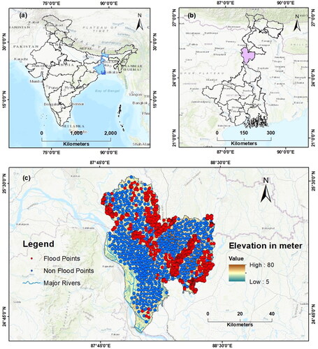
Table 1. Flood-affected areas of the Malda district based on DDMPM (2020-2021).

Sl. No.	Name of Blocks	Name of the G.P.	G.P wise Flood Prone Villages	Adjoining Rivers
1.	Harishchandrapur-II	Doulatnagar	Doulatnagar, Khidirpur and Mihahat	Mahananda and Fulhar
		Bhaluka	Hattichapa, Par Bhaluka
		Islampur	Basta, Bhajana, Chandpur, Chandipur Dakhin Bhakuria Imamnagar, Islampur, Khopakathi and Uttar Bhakuria
2.	Ratua-I	Debipur	Balupur, Debipur, Durgapur and Terashia	Fulhar, Koshi and Kalindri
		Mahanandatola	Badantola, Bajitpur, Bankutola, Dharmatola, Jagabandhutola, Janjalitola, Sambalpur and Sudamtola
		Bilaimari	Ajijtola, Dewanwala, Gangaramtola, Khasmahal, Nakkati, Nayabilaimari, Ramayanpur, and Ruhimari
		Kahala	Asutola, Haragobindapur, Kahala, Kalutola, Kamalpur, Narattampur and Suryapur
		Baharal	Baharal, Nimtalli, Sahapur Uttar and Sahapur Dakshin
3.	Manikchak	Gopalpur	Balutola, Elahitola (Part), Iswartola (Part), Kalitola, Kamaltipur, Nasutola (Part) and Sahabattola (Part)	Ganga and Fulhar
		Dharampur	Barabagan (Part), Sonapur and Wahedmara
		Manikchak	2No.Bridgepara, Chamatola. Darbaritola, Domhat, Jalalpur (part), Jotpatta, Madantola, Manikchak Ghat Bandh Para, Mankud, Narayanpur, Narayanpur Id Gaha Para, New Sonapur, Palpara, Rabidaspara, Ramnagar and Sibantola
		Dakshin Chandipur	Amintola, Bhabanitola, Bipintola, Bhabanathtola, Bhimtola, Bhojantola, Debutola, Durgaramtola, Duyani Char, Ganeshtola, Jaipaltola, Krishnatola, Lutihara, Mahendratola, Nabadiptola, Nayantola, Panchutola, Payaritola, Pulintola Bandh, Raghunathtola, Ratantola and Sukdevtola
		Hiranandapur	Anantalaltola, Bagedantola, Bagdukra, Baikunthatola Benutola Colony, Chabiltola, Debutola, Domontola, Gadai, Giridharotola, Gourangatola, Kalutontola, Lutihara, Mathurtola, Nanditola, Piyaritola and Rajkumartola.
		Nazirpur	Haripur (Part), Jitmanpur (Part), Laksikol (Part) and Laskarpur (Part)
4.	Kaliachak-II	Bangitola	Bintola, Chowdhutytola, Gosaihat, Jote Kostuty, Mahadevpur and Sadipur	Ganga and Fulhar
		Uttar Panchanandapur-I	Dolboxtola, Jinerditola, Laskaritola, Loharditola, Nasarattola, Paglaghat Bus Stand, Ramlaltola (part) and Sultantola
		Uttar Panchanandapur-II	Dhelfora, Jitnagar and Jugaltola
		Hamidpur	8 No. Spar Bandh, Chechrutola, Chumkitola, Etwaritola, Jatintola, Khatiakhana Char, Mathabhanga, Piaritola (East and West), Shibutola, Shripur colony, and Tofi
		Rajnagar	Bromottar and Nayagram Model
5.	Kaliachak-III	Birnagar-II	Asgarhajitola and Dinutola	Ganga and Fulhar
		Laxmipur	Ajimtola, Atartola, Bhangatol, Hajrattola, Jagantpur Mouza
		Krishnapur	Charsujapur, Kalitola, Mondai and Surenmandalpara
		Bakhrabad	Deonapur
		Kumbhira	Noornagar and Sabdalpur
		Pardeonapur-Sovapur	Dalpra, Golapman, Paranupnagar, Parlalpur and Shibpur

District Disaster Management Plan, Government of West Bengal, Office of the District Magistrate, Malda (2018, 2019–2020, 2020–2021) (http://wbdmd.gov.in/writereaddata/uploaded/DP/DPMalda57797.pdf).

2.2. Flood inventory map

The creation of a flood inventory map is an essential component in evaluating the outcomes of the studied region. Such information is indispensable in establishing flood risk regions by drawing on historical flood records. The primary objective of this study is to generate a flood inventory map utilizing historical flood data acquired from BHUVAN a geo-platform created by ISRO (Indian Space Research Organisation). Figure 1(c) illustrates the integration of the flood inventory map with the map of the study area. The study has identified a total of 1120 locations susceptible to flooding and 620 locations that are not prone to flooding, which will be subjected to further evaluation (Figure 2).

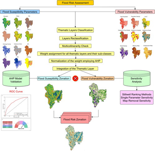
Figure 2. Methodological flowchart of the flood risk assessment.

2.3. Selection of the thematic layers

Multi-criteria decision-making (MCDM) methodology was employed to evaluate the flood risk zone area in the Malda district. The methodology employed RS and GIS techniques. The research classified the criteria into two primary groups, FS factors and flood vulnerability (FV) factors. A total of twelve parameters (n = 12) were selected for evaluating FS, while nine parameters (n = 9) were selected for assessing FV, as outlined below.

2.4. Flood susceptibility (FSP) and vulnerability (FVP) parameters

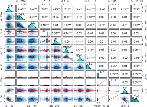
Elevation (Figure 3a) has a direct correlation with the potential for flooding events. Therefore, it has been regarded as a critical element of FS. Areas with lower elevations are more vulnerable to floods as a result of increased river flow and waterlogging conditions (Das 2018). The occurrence of flooding is dependent upon the sloping (Figure 3b) nature of the terrain, whereby a decrease in slope is positively correlated with an elevated probability of flooding (Sar et al. 2015; Das and Pardeshi 2017; Mitra and Das 2022). It is directly correlated with the flow rate, the volume of surface runoff, and the infiltration rate (Horton 1932; Ghosh and Kar 2018; Mitra et al. 2022). A significant susceptibility parameter is the TWI (Figure 3c). It quantifies the wetness of a landscape by incorporating topographic features (Das 2018; Souissi et al. 2019; Mitra et al. 2022). It primarily shows the spatial patterns of soil moisture in floodplain zone (Mitra et al. 2022). The topographic positioning index (TPI) (Figure 3d) refers to the variance in height between adjacent cells within a certain radius (Das 2018; Rahmati et al. 2019; Paul and Sarkar 2022). De Reu et al. (2013) and Mitra and Das (2022) made the first proposal due to the critical role of microtopographic variation in determining various hydrological parameters, such as water holding and flow velocity, TPI is used for FS research. The identification of vegetation coverage is commonly accomplished through the utilisation of the NDVI (Figure 3e) analysis (Mitra et al. 2022). Negative NDVI values indicate an area that is very prone to floods (Hidayah et al. 2022). The present research utilized the modified normalized difference water index (MNDWI) (Figure 3f) as an essential indicator for evaluating FS instead of the normalized difference water index (NDWI). The MNDWI recognized water bodies more accurately than the NDWI (Xu 2006). As a result, the metric MNDWI is very helpful for identifying locations with low-lying terrain. The drainage density (DD) (Figure 3g) of any region is proportional to the stream’s maximum flow (Horton 1932; Mitra and Das 2022). It directly affects runoff and infiltration capacity. As a result, it is strongly associated with FS. Regions characterised by a high density of drainage channels are associated with an increased likelihood of experiencing flooding events (Msabi and Makonyo 2021). One of the most important FS parameters for determining flood-prone locations is the distance from the river (DTR) (Figure 3h). Areas near rivers (i.e. active floodplain zones) are more prone to flooding compared to those located further away from rivers (Ghosh and Kar 2018; Mitra et al. 2022). The Stream Power Index (SPI) (Figure 3i) is widely recognised as the primary indicator of the erosive capacity of streams (Mitra et al. 2022). It has an influence on flood damage (Mitra et al. 2022) and is used to determine the most advantageous places for soil protection techniques (Mojaddadi et al. 2017; Das and Gupta 2021). Runoff and the volume of silt transported by streams in every location are connected to the sediment transport index (STI) (Figure 3j) (Rahmati et al. 2019; Das and Gupta 2021). In general, lower STI values are associated with extremely flood-prone terrain. Rainfall is a critical determinant of FV. High-increasing rainfall during a short period increases the likelihood of surface runoff and floods in any place. The modified fournier Index (MFI) (Figure 3k) is used to show how rainfall intensity varies between regions. A higher MFI score is associated with areas that are very prone to floods (Mitra et al. 2022). Lithology (Figure 3l) is inextricably linked to soil permeability, which influences floods. Variance in rock types has resulted in variations in surface hydrology (Mitra et al. 2022; Paul and Sarkar 2022). Areas with impermeable lithological structures facilitate runoff and thereby increase the likelihood of floods (Miller 1990; Edet and Okereke 1997; Msabi and Makonyo 2021). As a result, the lithological structure of the local area is considered a critical flood conditioning feature. Figure 4 shows the Pearson Correlational Matrix among the different flood susceptibility parameters.

Figure 3. Flood susceptibility conditioning parameters of the Malda district: (a) elevation, (b) slope, (c) Topographical wetness index (TWI), (d) Topographical positioning index (TPI), (e) normalized difference vegetation index (NDVI), (f) modified normalized difference water index (MNDWI), (g) drainage density, (h) distance to river, (i) Stream power index (SPI), (j) modified fourier index (MFI) and (k) lithology.

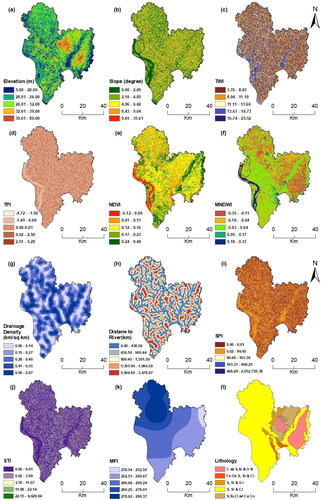
Figure 4. Pearson Correlational Matrix among the different flood susceptibility parameters.

The population (Figure 5a) is a critical factor in determining FV. Environmental vulnerability is magnified as a result of population growth. Hazards and disasters commonly occur in developing nations or third-world countries as a result of excessive population stress. The population density (Figure 5b) of a place has been regarded as another critical element, especially for determining the area’s pressure. It has been noted that locations with a high population density are more prone to floods (Ghosh and Kar 2018; Mitra et al. 2022). Land use is also regarded as a critical factor affecting infiltration, runoff, and evapotranspiration (Das and Gupta 2021). Thus, LULC (Figure 5c) has had a direct effect on any region’s hydrological characteristics. Specifically, the natural hydrological cycle has been interrupted in metropolitan areas because of shifting land-use patterns (Mitra et al. 2022; Paul and Sarkar 2022). As a result, the LULC factor contributes to flood hazards. In determining the vulnerability of an area, the proximity and availability of flood shelters (Figure 5d) and medical facilities (Figure 5e) are crucial factors (Hoque et al. 2019). Rapid access to flood shelters and medical services for all vulnerable individuals may considerably mitigate hazard outcomes. When victims are present, an adequate number of hospital beds and adequately trained personnel are required for effective hazard management (Das and Gupta 2021; Mitra et al. 2022; Paul and Sarkar 2022). Two characteristics relating to roads are examined, namely the distance to the road (Figure 5f) and the road density (Figure 5g). Education is a crucial component to consider when examining vulnerability. A highly educated populace employs more ways to deal with flooding; hence, they are more equipped to deal with floods (Ghosh and Kar 2018; Salazar-Briones et al. 2020; Mitra et al. 2022). As with literacy rates (Figure 5h), employment rates (Figure 5i) are critical indicators of a region’s vulnerability. The higher employment ratio indicates that the economy is strong enough to withstand physical vulnerabilities such as floods, droughts, and landslides. Figure 6 shows the Pearson Correlational Matrix among the different FV parameters. Figure 2 illustrates the methodology used to determine susceptibility, vulnerability, and risk zones.

Figure 5. Flood vulnerability conditioning parameters of the Malda district: (a)total population, (b) population density, (c) land use land cover (LULC), (d) distance to flood shelter, (e) distance to hospital, (f) distance to road, (g) road density, (h) illiteracy rate and (i) employment rate.

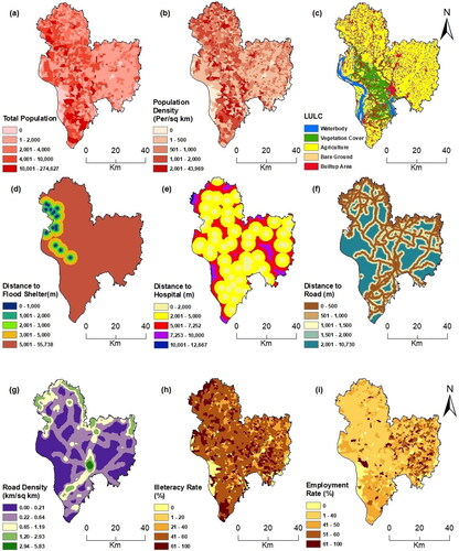
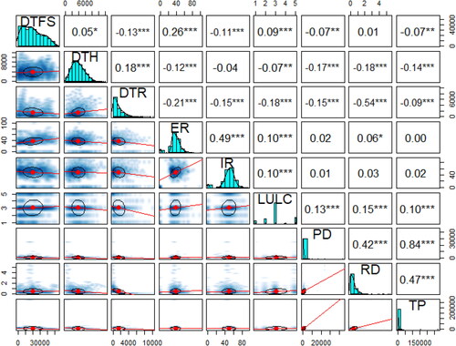
Figure 6. Pearson Correlational Matrix among the different flood vulnerability parameters.

2.5. Data collection and preparation of thematic maps

The objective of the current research was to systematically examine and establish the FS parameter (FSP) and FV parameter (FVP) through scientific means. This study utilized diverse thematic data layers obtained from credible sources and underwent processing within the ESRI ArcGIS 10.4.1 framework to attain the desired outcome. The USGS ASTER GDEM, a digital model of the Earth’s surface with a spatial resolution of 30 meters, was employed to produce various thematic layers, such as elevation, slope, TPI, TWI, SPI, and STI. The integration of these layers encompassed the entirety of the designated research locale and was subsequently demarcated for the study site, culminating in the calculation of multiple supplementary layers. The derivation of the drainage network was based on the ASTER GDEM dataset. The study utilized radiometrically corrected satellite images obtained from the USGS LANDSAT-8 to generate three distinct indices, namely NDVI, MNDWI, and LULC, simultaneously. The indices above were utilized for diverse computations. The modified fournier index (MFI) method was utilized to create a rainfall intensity map based on data collected by the Indian Meteorological Department (IMD) over 35 years, from 1986 to 2020. Collating data compiled thematic lithology layers from the BHUKOSH GSI (Geological Survey of India). The study acquired demographic and socio-economic information at the village level, such as total population, population density, illiteracy rate, and employment rate, from the District Census Handbook of Maldah District (DCHM) Census of India (2011). Following this, spatial distribution layers were created for each parameter. Spatial layers were generated to depict the proximity to the hospital, distance to the road, and road density. The data utilized for this purpose was obtained from the OpenStreetMap website. The distance to the flood shelter layer was created using data sourced from the District Disaster Management Plan for the period spanning 2020-2021. Table 2 represents a comprehensive summary of the origins and explanations of the parameters employed in the susceptibility and vulnerability zonation.

Table 2. Source and description of the parameters used in susceptibility and vulnerability zonation.

Parameters	Descriptions	Source
Elevation, Slope, TWI, TPI, SPI, STI, Drainage Density and Distance to River	Derived from ASTER DEM (30m*30m) and prepared the thematic layer using ArcGIS 10.4.1	United States of Geological Survey (USGS) Retrieved from: (https://earthexplorer.usgs.gov)
NDVI, MNDWI and LULC	Landsat-8 OLI/TIRS, (30m*30m)	United States of Geological Survey (USGS) Retrieved from: (https://earthexplorer.usgs.gov)
Rainfall Intensity using MFI	Gridded rainfall (0.25*0.25) NetCDF File	Indian Meteorological Department (IMD) Retrieved from: (http://www.imdpune.gov.in)
Lithology	Digital lithological map of the district	Geological Survey of India (GSI) Retrieved from: (http://bhukosh.gsi.gov.in/)
Total population, Population density, Illiteracy rate and Employment rate	Obtaining the village-level data from Census of India, 2011	Office of the Register General & Census Commissioner, India Retrieved from: (http://censusindia.gov.in/)
Distance to flood shelter	Adopting the data from DDMPM (2020-2021)	District Disaster Management Plan of Malda District, West Bengal (2020-2021), Retrieved from: (http://wbdmd.gov.in/writereaddata/uploaded/DP/DPMalda59094.pdf)
Distance to hospital, Distance to road, and Road density	Adopting the data from OpenStreetMap	OpenStreetMap Retrieved from: (www.openstreetmap.org)

The TWI layer is derived from the ASTER GDEM dataset utilizing the formula outlined in Equation 1(1) $$\mathit{TWI}=Ln\left(\frac{a}{\tan \hspace{0.17em}B}\right)\mathrm{ }$$(1) (Beven and Kirkby 1979; Mitra et al. 2022), (1) $$\mathit{TWI}=Ln\left(\frac{a}{\tan \hspace{0.17em}B}\right)\mathrm{ }$$(1)

 Where, ‘the variables $\alpha$ and $B$ pertain to the catchment area and slope, respectively, of the region under investigation, respectively. Furthermore, here $a= \frac{A}{L},$ where the variable $A$ represents the entirety of the basin’s area, and denotes the length of the contour being analysed’ (Beven and Kirkby 1979; Mitra et al. 2022).

The TPI map was utilised to facilitate the evaluation of FS through the utilisation of Equation 2(2) $$\mathit{TPI}=z_0-{\tilde{z}}_i\mathrm{ }$$(2) and Equation 3(3) $${\tilde{z}}_i=\frac{1}{n_R}\sum _{i\in R}{Z}_i\mathrm{ }$$(3) . Furthermore, the TPI was evaluated within the ArcGIS platform utilizing the ‘land facet corridor designer tool’ (Jenness et al. 2013; Mitra et al. 2022). (2) $$\mathit{TPI}=z_0-{\tilde{z}}_i\mathrm{ }$$(2) (3) $${\tilde{z}}_i=\frac{1}{n_R}\sum _{i\in R}{Z}_i\mathrm{ }$$(3)

Both NDVI and MNDWI are determined from satellite imagery using Equation 4(4) $$\mathit{NDVI}=\frac{\mathit{NIR}-\mathit{Red}\mathrm{ }}{\mathit{NIR}+\mathit{Red}\prime }\mathrm{ }$$(4) and Equation 5(5) $$\mathit{mNDWI}=\frac{\mathit{Green}-\mathit{MIR}}{\mathit{Green}+\mathit{MIR}\prime }$$(5) , respectively. These equations are utilized to accurately calculate the values of these important indicators, which provide insights into vegetation and water content in the given area (Xu 2006; Mitra et al. 2022): (4) $$\mathit{NDVI}=\frac{\mathit{NIR}-\mathit{Red}\mathrm{ }}{\mathit{NIR}+\mathit{Red}\prime }\mathrm{ }$$(4) (5) $$\mathit{mNDWI}=\frac{\mathit{Green}-\mathit{MIR}}{\mathit{Green}+\mathit{MIR}\prime }$$(5)

Where, ‘$\mathit{Red}$ signifies red band, $\mathit{Green}$ signifies green band, $\mathit{MIR}$ signifies middle infra-red band, and $\mathit{NIR}$ signifies near-infrared band’. In addition to the susceptibility parameters, another important factor to consider is the STI, which can be calculated using Equation 6(6) $$\mathit{STI}=\left[\frac{{\left(\frac{F_a}{\delta x}\right)}^2}{{\left(\frac{\mathit{Sig n }(S_{a)}}{\delta y}\right)}^2}\right]$$(6) . Furthermore, the SPI can be derived from Equation 7(7) $$\mathit{SPI}=Ai\times \tan \beta$$(7) , (Mitra et al. 2022) as quantified below: (6) $$\mathit{STI}=\left[\frac{{\left(\frac{F_a}{\delta x}\right)}^2}{{\left(\frac{\mathit{Sig n }(S_{a)}}{\delta y}\right)}^2}\right]$$(6) (7) $$\mathit{SPI}=Ai\times \tan \beta$$(7)

Where, ‘$F_a$ represents the flow accumulation and $S_a$ represents the slope raster, derived from ASTER GDEM, and ${\delta }_x$ and ${\delta }_y$ represents the constant. $A_i$ Represents the specific area and $\tan \beta$ represents the gradient’. MFI is also used by obtaining the value from the Equation 8(8) $$\mathit{MFI}=\sum _{i=1}^{12}\frac{P_i^2}{P\prime }$$(8) (Mitra and Das 2022; Mitra et al. 2022): (8) $$\mathit{MFI}=\sum _{i=1}^{12}\frac{P_i^2}{P\prime }$$(8)

Where, ‘P_i represents to the average amount of precipitation in a month, while $P\prime$ represents the average amount of precipitation in a year’.

Drainage density calculated as shown Equation 9(9) $$Dd=\sum _{i=1}^{i=n}\frac{D_i}{A}\left({km}^{-1}\right)$$(9) (Mitra and Das 2022; Mitra et al. 2022) (9) $$Dd=\sum _{i=1}^{i=n}\frac{D_i}{A}\left({km}^{-1}\right)$$(9)

‘Where, $\sum D_i$ is the total length of the stream in the grid (km) and $A$ is the grid area (km²)’.

ArcGIS’s ‘Euclidean distance’ tool is used to build all spatial layers, including those showing the distance to rivers, flood shelters, hospitals, and roads. This drainage and road density map was created using the ‘line density’ tool on the ArcGIS environment. All raster layers were resampled to 30 m resolution using the ‘resample’ tool on the GIS platform.

2.6. Multi-collinearity assessment

The efficacy of the multi-collinearity test was ascertained based on its non-detrimental impact on the predictiveness and dependability of the model. The process of evaluating FS and vulnerability modelling entails the utilisation of the multicollinearity test, which involves identifying a linear correlation among the variables. There exists a notable correlation among various independent variables, which can be employed to discern independent variables that exhibit a strong correlation. The present study employed the variance inflation factor (VIF) method for the purpose of investigation. The Variance Inflation Factor (VIF) was calculated utilising the methodology outlined by Meyer et al. (2012). To validate this, a linear regression analysis uses an input parameter ($x_i$) as the independent variable and the other input variables as dependent variables ($y_i$). The $R^2$ value is then determined ($R{}_i{}^2$). Additionally, using Equation 10(10) $$\text{Tolerance of the ith predictor variable}\left(T_i\right)=1-R_i^2\mathrm{ }$$(10) and Equation 11(11) $$\text{VIF of the ith predictor variable }\left({\mathit{VIF}}_i\right)=\frac{1}{T_i}$$(11) , this value determines the input variable’s tolerance (TOL) and variance inflation factor (VIF) (Mukherjee and Singh 2020; Mitra et al. 2022). (10) $$\text{Tolerance of the ith predictor variable}\left(T_i\right)=1-R_i^2\mathrm{ }$$(10) (11) $$\text{VIF of the ith predictor variable }\left({\mathit{VIF}}_i\right)=\frac{1}{T_i}$$(11)

The process is repeated for each parameter, and tolerance and VIF values are computed for each input parameter. A tolerance of <0.10 or VIF of >1.0 indicates multicollinearity problems (Naghibi et al. 2017; Maiti and Mandal 2019; Mukherjee and Singh 2020; Mitra et al. 2022). For this evaluation, thematic layers with tolerance levels of less than 0.10 or VIF values >1.0 has been calculated.

2.7. Weighting and ranking by AHP

AHP is a powerful approach that employs expert opinions in a GIS environment to analyze multiple factors and facilitate decision-making (Mitra et al. 2022). Saaty (1977, 1980, 1987, 1990, Saaty 2006) developed AHP as a practical decision-making technique that involves creating a hierarchy of elements and assigning weights to each aspect to reduce the complexity of the decision-making process. To achieve an accurate outcome, assigning appropriate weights, weighting, and normalizing each parameter is critical for providing correct findings in AHP (Sener et al. 2010; Rahmati et al. 2014; Maity and Mandal 2017; Saha 2017; Zeng and Huang 2017; Yin et al. 2018; Biswas et al. 2022; Mitra et al. 2022). Saaty’s scale of significance assigns a value of 1 to ‘equal importance’ and a value of 9 to ‘extreme importance’ (Table 3).

Table 3. Saaty’s scale of relative importance.

Numerical Value	Definition
1	Equal importance
2	Equal to moderate importance
3	Moderate importance
4	Moderate to strong importance
5	Strong importance
6	Strong to very strong importance
7	Very strong importance
8	Very to extremely strong importance
9	Extreme importance
1/1 to 1/9	Reciprocal values

This study employs the AHP method to assign significance to FS and vulnerability indicators. Despite the availability of alternative techniques, the AHP approach is widely recognized as the most effective means of determining weights in FS and vulnerability assessment due to its consistent, efficient, and cost-effective outcomes. Utilizing the AHP method, expert opinions, field experience, and extensive literature reviews were used to assign weights to all twenty-one factors (n = 12 for FS and n = 9 for FV). This approach has been previously employed by Danumah et al. (2016), Seejata et al. (2018), Sharir et al. (2019), Swain et al. (2020), Roy et al. (2021), Biswas et al. (2022), and Hasanuzzaman et al. (2022). Discover how to accurately calculate the Pairwise comparison matrix for various thematic layers and evaluate their consistency with the tried-and-true steps outlined by Mitra et al. (2022). The supplementary material (SM) contains Tables SM1 and SM4, which present the pairwise comparison matrices, and Tables SM2 and SM5, which illustrate the normalized vector representation indicating FS and vulnerability aspects for the respective thematic layers.

2.8. Consistency checks

To ensure the consistency of data obtained through this method, the degree of consistency $CR$ is calculated using Equation 12(12) $$CR=\frac{CI}{RI}\mathrm{ }$$(12) . (12) $$CR=\frac{CI}{RI}\mathrm{ }$$(12)

Based on Saatty (1977, 1980, 1987, 1990 and 2006) an analysis can be carried out if the CR value is below 0.10. The current analysis yielded a CR value below 0.10 for both susceptibility and vulnerability factors, suggesting that the analysis was effective. If the CR value exceeds 0.10, it is necessary to revise the analysis from the outset to identify the origin of the problem within the matrix. (Saatty 1977, 1980, 1987, 1990, 2006; Vargas 1990). For various n values, the RCI values are constant, as shown in Table 4 based on Saaty and Vargas (1991), and CI is calculated as follows:

Table 4. Random index (RI) to check the consistency ratio for different matrices (Saaty and Vargas 1991).

1	2	3	4	5	6	7	8	9	10	11	12	13	14	15
0	0	0.58	0.9	1.12	1.24	1.32	1.41	1.45	1.49	1.51	1.48	1.56	1.57	1.59

Additionally, ‘the consistency index CI is calculated using Equation 13(13) $$CI=\frac{\left({\lambda }_{\max }-n\right)}{\left(n-1\right)}$$(13) , where λ_max represents the maximum eigenvalue of the matrix’. (13) $$CI=\frac{\left({\lambda }_{\max }-n\right)}{\left(n-1\right)}$$(13)

If the ‘degree of consistency CR is less than 0.10, the result is considered sufficiently accurate, and no further adjustments are necessary. The λ_max is calculated using the Eq. 14(14) $${\lambda }_{\max }=\sum _{i=1}^n\left(W_i\times \frac{P_i}{{\sum }_{i=1}^n{P}_i}\right)\mathrm{ }$$(14) ’: (14) $${\lambda }_{\max }=\sum _{i=1}^n\left(W_i\times \frac{P_i}{{\sum }_{i=1}^n{P}_i}\right)\mathrm{ }$$(14)

Where, ‘λ_max is denoted by the principal or eigenvalue of the pairwise comparison matrix’.

2.9. Mapping of flood susceptibility, vulnerability, and flood risk zonation

The FS and vulnerability parameters were weighted using the AHP methodology based on the respective severity of each parameter. The weights were employed in the cartographic representation of the ArcGIS platform, and the Spatial Analyst tool was utilized in conjunction with the weighted overlay technique. Equation 15(15) $$\mathit{FSZ}=\sum _{i=1}^n{W}_i^S\times R_i^S$$(15) and Equation 16(16) $$\mathit{FVZ}=\sum _{i=1}^n{W}_i^V\times R_i^V$$(16) are utilized to calculate the FSZ and FVZ, respectively. (15) $$\mathit{FSZ}=\sum _{i=1}^n{W}_i^S\times R_i^S$$(15)

Where, ‘FSZ stands for the FS zonation, $W_i^S$ represents susceptibility parameters’ weights, $R_i^S$ represents the rank of susceptibility parameters’. (16) $$\mathit{FVZ}=\sum _{i=1}^n{W}_i^V\times R_i^V$$(16)

Where, ‘FVZ stands for the FV zonation, $W_i^V$ represents vulnerability parameters’ weights, $R_i^V$ represents the rank of vulnerability parameters’.

The primary objective of the present study is to develop a flood risk zonation (FRZ) model. The desired outcome was achieved by multiplying the flood susceptibility zonation (FSZ) and flood vulnerability zonation (FVZ) maps using Equation 17(17) $$\mathit{FRZ}=\mathit{FSZ}\times \mathit{FVZ}$$(17) . (17) $$\mathit{FRZ}=\mathit{FSZ}\times \mathit{FVZ}$$(17)

2.10. Assessment of the AHP method

The prioritization of weightage holds significant importance in the AHP methodology. Consequently, it is imperative to employ sensitivity analysis to validate the weights allocated by AHP. The present investigation employed several sensitivity analysis techniques, including single parameter sensitivity, Stillwell ranking methods, and map removal sensitivity analysis.

2.10.1. The Stillwell ranking method

The two algorithms that make up the Stillwell ranking approach are the Reciprocal Rank function and the Rank sum weight function.

Rank sum weight function (Stillwell et al. 1981): (18) $$Wj\left(RS\right)=(n-rj+1)/\sum _{k=1}^n\left(n-rk+1\right)=2\left(n+1-r\right)/n\left(n+1\right)$$(18)

Reciprocal Rank function (Stillwell et al. 1981): (19) $$Wj\left(RR\right)=\frac{1}{rj}/\sum _{k=1}^n\left(\frac{1}{rk}\right)\mathrm{ }$$(19)

2.10.2. Single parameter sensitivity analysis

The effectiveness of each thematic layer in the FSZ and FVZ maps is evaluated using single parameter sensitivity analysis. This involves comparing the weights assigned to each thematic layer with the empirical weights assigned to the same layer in previous studies (Napolitano & Fabbri, 1996; Fenta et al. 2014; Thapa et al. 2018; Mukherjee and Singh 2020; Mitra et al. 2022). This study determined the effective weighting factor for FSZ and FVZ for each thematic layer using Equation 20(20) $$W_i=\frac{P_r{P}_w}{{\mathit{FSZ}}_i}\times 100$$(20) and Equation 21(21) $$W_i=\frac{P_r{P}_w}{{\mathit{FVZ}}_i}\times 100$$(21) . (20) $$W_i=\frac{P_r{P}_w}{{\mathit{FSZ}}_i}\times 100$$(20) (21) $$W_i=\frac{P_r{P}_w}{{\mathit{FVZ}}_i}\times 100$$(21)

Where, ‘W_i represents effective weight, P_r and P_w represents rates and weight values of each thematic layer, FSZ_i represents FS zonation and FVZ_i represents FV zonation’.

2.10.3. Map removal sensitivity analysis

The assessment of map removal sensitivity is a crucial sensitivity analysis investigating the impact of removing any of the thematic layers employed in predicting FSZ and FVZ maps. This approach involves the stepwise removal of thematic layers (Lodwick et al. 1990; Fenta et al. 2014; Thapa et al. 2018; Mukherjee and Singh 2020; Mitra et al. 2022). With each layer removed, a new map is generated by overlaying the remaining layers, creating new FSZ and FVZ maps. The sensitivity index is then calculated using Equation 22(22) $${SI}_i=\frac{\left|\left(\frac{\mathit{FSZ}}{N}\right)-\left(\frac{\mathit{FSZ}\prime }{n}\right)\right|}{\mathit{FSZ}}\times 100$$(22) and Equation 23(23) $${SI}_i=\frac{\left|\left(\frac{\mathit{FVZ}}{N}\right)-\left(\frac{\mathit{FVZ}\prime }{n}\right)\right|}{\mathit{FVZ}}\times 100\mathrm{ }$$(23) . (22) $${SI}_i=\frac{\left|\left(\frac{\mathit{FSZ}}{N}\right)-\left(\frac{\mathit{FSZ}\prime }{n}\right)\right|}{\mathit{FSZ}}\times 100$$(22) (23) $${SI}_i=\frac{\left|\left(\frac{\mathit{FVZ}}{N}\right)-\left(\frac{\mathit{FVZ}\prime }{n}\right)\right|}{\mathit{FVZ}}\times 100\mathrm{ }$$(23)

Where, ‘SI_i indicates the sensitivity index linked to each theme layer that is removed, FSZ and FVZ respectively, display the FS and vulnerability zones for all thematic layers, Zones of vulnerability and FS for one excluded thematic layer were displayed in FSZ’ and FVZ’, N represents number of thematic layers used to generate the FSZ and FVZ maps, and n represents number of thematic layers considered to generate the FSZ’ and FVZ’ maps’.

2.11. Accuracy assessment of the model

Numerous methods exist for validating MCDA models; however, data validation is regarded as a crucial step in ensuring the precision of any model after its creation. This study validated the FSZ maps displaying the balance between sensitivity and specificity using ROC and AUC (Area under the ROC Curve) techniques (Hanley and McNeil 1982). The y-axis of the two-dimensional ROC plot represents sensitivity, whereas the x-axis represents 1- specificity. Equation 24(24) $$x=1-\mathrm{specificity}=1-\left[\frac{TN}{\left(TN+FP\right)}\right]$$(24) and Equation 25(25) $$y=\mathit{sensitivity}=\left[\frac{TN}{\left(TP+FN\right)}\right]$$(25) depict the features of the x and y axes, respectively. In these equations, TN denotes true negative, FP denotes to false positive, TP denotes true positive, and FN denotes false negative (Swets 1988; Mitra and Das 2022; Mitra et al. 2022; Sachdeva and Kumar 2022). (24) $$x=1-\mathrm{specificity}=1-\left[\frac{TN}{\left(TN+FP\right)}\right]$$(24) (25) $$y=\mathit{sensitivity}=\left[\frac{TN}{\left(TP+FN\right)}\right]$$(25)

The Area Under the Curve (AUC) was employed to evaluate the effectiveness of the AHP method within the study region. The model was validated using flood and non-flood data points from the district. AUC-ROC values range between 0 and 1, where a score of 1 signifies an outstanding correlation, while a score of 0 indicates a weak association between AUC and the prediction rate.

3. Multicollinearity checks

The multicollinearity testing for the vulnerability and susceptibility indicators in the study utilized 1000 randomly selected sites. The tested 12 FS factors’ collinearity results showed no substantiation of a multicollinearity issue. All susceptibility factors have a VIF and tolerance value of <10 and > 0.1, respectively. Additionally, the eigenvalue and condition index of all susceptibility-related considerations demonstrate the presence of multicollinearity (Table 5). The variance proportion Table 6 only contains one predictor, the MFI for dimension 12, and it exhibits a high value (> 0.90), which does not perpetuate the multicollinearity, as demonstrated by Table 6.

Table 5. Multicollinearity Statistics of flood susceptibility and vulnerability parameters.

SP	E	S	TWI	TPI	NDVI	MNDWI	DD	DR	SPI	STI	MFI	L
Tolerance	0.579	0.781	0.555	0.721	0.790	0.754	0.540	0.538	0.161	0.151	0.991	0.945
VIF	1.727	1.280	1.802	1.386	1.266	1.327	1.853	1.858	6.216	6.626	1.009	1.058
SP: Susceptibility Parameters, E: Elevation, S: Slope, TWI: Topographic Wetness Index, TPI: Topographic Position Index, NDVI: Normalized Difference Vegetation Index, MNDWI: Modified Normalized Difference Water Index, DD: Drainage Density, DR: Distance to River, SPI: Stream Power Index, STI: Sediment Transport Index, MFI: Modified Fourier Index, L: Lithology.
VP	TP	FP	PD	CD	LR	ILR	DFS	DH	LULC	ER	RD	DTR
Tolerance	0.310	0.003	0.111	0.004	0.559	0.517	0.803	0.887	0.941	0.409	0.501	0.594
VIF	3.220	286.659	8.989	229.811	1.790	1.933	1.246	1.127	1.063	2.448	1.997	1.683

VP: Vulnerability Parameters, TP: Total Population, FP: Female Population, CD: Child Population, LR: Literacy Rate, ILR: Illiteracy Rate, DFS: Distance to Flood Shelter, DH: Distance to Hospital, LULC: Land Use Land Cover, ER: Employment Rate, RD: Road Density, DTR: Distance to Road.

Table 6. Multi-collinearity diagnosis of flood susceptibility and vulnerability parameters.

Dimension	Susceptibility		Vulnerability
	Eigenvalue	Condition Index	Eigenvalue	Condition Index
1	6.181	1.000	7.556	1.000
2	1.885	1.811	2.547	1.722
3	1.023	2.458	0.756	3.162
4	0.886	2.641	0.305	4.978
5	0.822	2.743	0.257	5.426
6	0.479	3.591	0.198	6.177
7	0.301	4.531	0.138	7.395
8	0.152	6.370	0.100	8.695
9	0.101	7.830	0.090	9.182
10	0.093	8.173	0.036	14.511
11	0.060	10.130	0.016	21.618
12	0.016	19.966	0.002	64.907

A strong correlation between the parameters ‘female population’ and ‘child under 6 years’ has been sustained in the vulnerability parameters situation. According to the collinearity results, both parameters show VIF, and the tolerance values are >10 and <0.1. (Table 5). Dimensions 10 and 11 have eigenvalues that are nearer to 0, which suggests multicollinearity. There is more than one predictor with a variance proportion of >0.90 and the observed condition matrix for both dimensions is higher than 15. (Table 6). To avoid this collinearity, one substantially correlated parameter from the two (i.e. ‘female population’ and ‘child under 6 years’) should be eliminated. For this vulnerability analysis, only 9 specified criteria have been considered.

4. Results

4.1. Flood susceptibility zonation (FSZ)

This present research aims to examine the variability in FS intensity throughout the Malda District in West Bengal. Before implementing the AHP model, the Consistency Ratio (CR) for each thematic layer and its respective subclasses was calculated (Table 7). Table SM3, presented in the electronic supplementary material, displays the rating, lambda max, CI, and CR values that correspond to various sub-criteria for each Flood Susceptibility class. The results indicated that the judgment matrices were consistent, with values below 0.10 (Table 8). The study area was analyzed using ArcGIS software to create FS maps for individual pixels. The maps were generated based on the weight and normalized rank of selected criteria for each criterion. The maps aimed to illustrate the spatial variability of flood magnitude across the district. Furthermore, the ArcGIS platform has incorporated twelve thematic layers of FS parameters that have been reclassified with their respective weights. Consequently, the district’s ultimate Flood Susceptibility Zonation (FSZ) map (Figure 7a) was generated utilizing the ‘weighted overlay method’. The resultant map derived from the analysis has been categorized into five distinct classes of FS: very low, low, moderate, high, and very high levels. The distribution of these categories across various methods is presented in Table SM7 of the electronic supplementary material. The Tal and Diara region in the district’s western half is included in the results, which show that the FS there is quite serious. The Ganga, Fulhar, Kalindi, and Mahananda rivers’ younger, low-lying flood plains are particularly susceptible to floods. The flood threat has increased due to factors including lower altitude, gentle slope, high concentration of rainfall, higher drainage density, excessive increase in water level during the rainy season, siltation of riverbeds, and back thrust action at river confluences. In contrast, the Barind region in the eastern half of the district has a very low level of flood threat, except for the Tangon and Punarbhava riverine flood plains. The FS level ranges from moderate to low in the eastern half because it is relatively elevated, has a moderate slope, and has an undulating landscape. The most sensitive areas of the district are the Harischandrapur-I & II, Kaliachak-II & III, Manikchak and Ratua-I & II blocks, which are situated between the Ganga, Fulahar, Kalindi, and Mahananda rivers. Meanwhile, Bamangola, Gajole, Habibpur, and Old Malda blocks, which are situated between the Mahananda and Tangon rivers and the Punarbhava and Tangon interfluves, have moderate susceptibility.

Figure 7. (a) Flood susceptibility zonation, (b) flood vulnerability zonation, and (c) flood risk zonation map of Malda district.

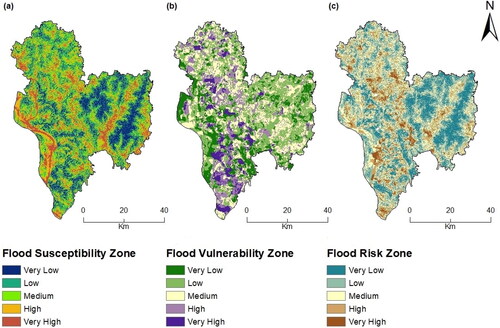
Table 7. AHP Table for flood susceptibility Zone analysis.

Parameters	AHP Weight	Reclass	Class Range	Flood Level	Area in Sq. Km	Area in %	Rating
Elevation	0.267	1	5 − 20	Very High	719.75	19.63	0.416
		2	21 − 26	High	1512.19	41.25	0.262
		3	27 − 32	Medium	874.30	23.85	0.161
		4	33 − 39	Low	425.72	11.61	0.099
		5	40 − 80	Very Low	134.01	3.66	0.062
Slope	0.192	1	0.00 − 2.09	Very High	1054.44	28.76	0.444
		2	2.10 − 4.05	High	1211.89	33.06	0.262
		3	4.06 − 6.42	Medium	901.48	24.59	0.153
		4	6.43 − 9.64	Low	399.86	10.91	0.089
		5	9.65 − 35.61	Very Low	98.30	2.68	0.053
TWI	0.087	1	3.76 − 8.03	Very Low	1234.81	33.68	0.053
		2	8.04 − 11.10	Low	705.11	19.23	0.089
		3	11.11 − 13.66	Medium	842.15	22.97	0.153
		4	13.67 − 16.73	High	726.90	19.83	0.262
		5	16.74 − 25.52	Very High	157.00	4.28	0.444
TPI	0.015	1	−4.72 − 1.50	Very High	983.01	26.74	0.489
		2	−1.49 − 0.00	High	696.84	18.96	0.261
		3	0.00 − 0.01	Medium	327.53	8.91	0.138
		4	0.02 − 2.50	Low	1610.11	43.81	0.073
		5	2.51 − 5.29	Very Low	58.09	1.58	0.038
NDVI	0.028	1	−0.12 − 0	Very High	663.80	18.11	0.416
		2	0.01 − 0.11	High	1473.97	40.21	0.262
		3	0.12 − 0.16	Medium	907.42	24.75	0.161
		4	0.17 − 0.23	Low	436.94	11.92	0.099
		5	0.24 − 0.40	Very Low	684.50	18.67	0.062
MNDWI	0.063	1	−0.35 − 0.11	Very Low	1211.45	33.05	0.056
		2	−0.10 − 0.04	Low	1386.03	37.81	0.096
		3	−0.03 − 0.04	Medium	185.29	5.05	0.157
		4	0.05 − 0.17	High	198.69	5.42	0.257
		5	0.18 − 0.37	Very High	894.33	24.40	0.434
Drainage Density	0.123	1	0.00 − 0.14	Very Low	727.86	19.85	0.050
		2	0.15 − 0.27	Low	894.33	24.40	0.088
		3	0.28 − 0.40	Medium	955.64	26.07	0.151
		4	0.41 − 0.55	High	729.40	19.90	0.259
		5	0.56 − 0.87	Very High	358.70	9.78	0.454
Distance from the River	0.122	1	0.00 − 436.58	Very High	1015.75	27.71	0.503
		2	436.59 − 900.44	High	950.41	25.93	0.260
		3	900.45 − 1,391.59	Medium	804.43	21.94	0.134
		4	1,391.60 − 1,964.59	Low	622.27	16.97	0.068
		5	1,964.60 − 3,478.97	Very Low	273.07	7.45	0.035
SPI	0.015	1	0.00 − 0.01	Very High	1340.15	36.56	0.503
		2	0.02 − 99.65	High	2155.67	58.80	0.260
		3	99.66 − 193.30	Medium	51.23	1.40	0.134
		4	193.31 − 498.25	Low	47.11	1.29	0.068
		5	498.26 − 2,052,755.38	Very Low	71.81	1.96	0.035
STI	0.015	1	0.00 − 0.01	Very High	2156.88	58.84	0.503
		2	0.02 − 3.69	High	1143.47	31.19	0.260
		3	3.70 − 11.07	Medium	268.96	7.34	0.134
		4	11.08 − 22.14	Low	49.92	1.36	0.068
		5	22.15 − 8,420.94	Very Low	46.74	1.28	0.035
MFI	0.044	1	239.61 − 252.35	Very Low	70.52	1.92	0.053
		2	252.36 − 260.71	Low	1003.81	27.38	0.089
		3	260.72 − 269.27	Medium	1308.32	35.69	0.153
		4	269.28 − 278.03	High	882.20	24.06	0.262
		5	278.04 − 290.37	Very High	401.08	10.94	0.444
Lithology	0.028	1	CLAY WITH SAND, SILT, AND IRON NODULE	Low	492.70	13.44	0.070
		2	FEEBLY OXIDIZED SAND, SILT, AND CLAY	Very High	59.87	1.63	0.501
		3	SAND, SILT & GRAVEL	Medium	134.54	3.67	0.159
		4	SAND, SILT, AND CLAY	Very Low	2648.23	72.24	0.035
		5	SAND, SILT, CLAY WITH CALCAREOUS CONCRETIONS	High	330.59	9.02	0.235

Table 8. Consistency check of aggregated for flood hazard in the Malda district.

Lambda Max	N	Consistency Index	Consistency Ratio
13.26	12	0.115	0.077

4.2. Flood vulnerability zonation (FSZ)

This investigation evaluated vulnerability by considering multiple factors contributing to its escalation, such as population distribution, growth and concentration, population density, and unorganized land use pattern. These factors were placed in the numerator, while resilient components such as infrastructure, transportation, and communication facilities were included in the denominator, as they can reduce the vulnerability. Among the nine parameters that were taken into account, it was found that five of them, specifically total population, population density, land use, land cover, distance to flood shelter, and distance to hospital, (Table 9) played a significant role in the creation of the Final Vulnerability Zonation (FVZ) map (Figure 7b), accounting for over 80% of its development. The regions characterized by high population density, urbanization, and agricultural land use near rivers are at an increased risk of flooding, particularly in areas with high to extremely high FV. The district’s composite vulnerability map was generated by assigning normalized rankings to each feature class and utilizing the normalized AHP-driven individual feature weights in the ArcGIS software (Table 10). For different sub-criteria for each Flood Vulnerability class, Table SM6 in the electronic supplementary material shows the corresponding rating, lambda max, CI, and CR values. The cartographic output was categorized into five levels of vulnerability: very low, low, moderate, high, and very high. The electronic supplementary material Table SM8 displays the spatial distribution of these classes utilizing various techniques. The areas with high vulnerability are characterized by rapid population growth, high settlement density, agricultural concentration along riverbanks, low to moderate literacy rate, low to moderate employment rate, and inadequate infrastructure to deal with natural hazards. Malda, Tal and Diara areas are the most vulnerable to natural hazards, except for Kaliachak-II block, which has moderate to low vulnerability due to its moderate population growth, settlement density, high literacy rate, and better employment rate. In the eastern part of the district, the composite vulnerability score is moderate to low due to the moderate to low population growth rate and density and high literacy rate. Additionally, regions adjacent to national and state roads have shown moderate to low vulnerability due to increased accessibility and connectivity.

Table 9. AHP Table for flood vulnerability Zone analysis.

Parameters	AHP Weight	Reclass	Class Range	Flood Level	Area in Sq. Km	Area in %	Rating
Total Population	0.235	1	0	Very Low	225.94	6.16	0.044
		2	1 − 2,000	Low	1612.14	43.98	0.084
		3	2001 − 4000	Moderate	682.51	18.89	0.148
		4	4,001 − 10,000	High	851.43	23.23	0.256
		5	>10000	Very High	283.93	7.75	0.467
Population Density	0.235	1	0	Very Low	225.94	6.16	0.044
		2	1 − 500	Low	1325.64	36.16	0.084
		3	501 − 1,000	Moderate	1068.57	29.15	0.148
		4	1.001 − 2.000	High	776.45	21.18	0.256
		5	>2000	Very High	269.36	7.35	0.467
Illiteracy Rate	0.038	1	0	Very Low	227.44	6.21	0.035
		2	1 − 20	Low	20.32	0.55	0.068
		3	21 − 40	Moderate	467.70	12.76	0.134
		4	41 − 60	High	2262.73	61.75	0.260
		5	61 − 100	Very High	686.11	18.72	0.503
Distance to Flood Shelter	0.096	1	0 − 1,000	Very Low	48.08	1.31	0.048
		2	1001 − 2000	Low	110.45	3.01	0.085
		3	2,001 − 3,000	Moderate	121.88	3.32	0.148
		4	3,001 − 5,000	High	234.64	6.40	0.234
		5	5,001 − 55,738	Very High	3150.90	85.95	0.485
Distance to Hospital	0.096	1	0 − 2000	Very Low	645.71	17.61	0.049
		2	2,001 − 3,000	Low	683.52	18.65	0.082
		3	3,001 − 5,000	Moderate	1347.53	36.76	0.149
		4	5001 − 10000	High	973.04	26.54	0.267
		5	10,001 − 12,667	Very High	16.15	0.44	0.454
LULC	0.153	1	Waterbody	Very Low	285.28	7.78	0.035
		2	Vegetation Cover	Moderate	501.44	13.68	0.134
		3	Agricultural Field	High	2167.42	59.12	0.260
		4	Bare Ground	Low	68.70	1.87	0.068
		5	Built-up Area	Very High	643.10	17.54	0.503
Employment Rate	0.027	1	0	Very High	222.81	6.08	0.467
		2	1 − 40	High	1959.26	53.44	0.256
		3	41 − 50	Moderate	1001.20	27.31	0.148
		4	51 − 60	Low	337.81	9.21	0.084
		5	61 − 100	Very Low	141.24	3.85	0.044
Road Density	0.060	1	0.00 − 0.21	Very High	1371.73	37.42	0.426
		2	0.22 − 0.64	High	1484.77	40.50	0.259
		3	0.65 − 1.19	Moderate	538.31	14.68	0.159
		4	1.20 − 2.93	Low	251.75	6.87	0.097
		5	2.94 − 5.83	Very Low	19.39	0.53	0.059
Distance to Road	0.060	1	0-500	Very Low	1153.67	31.47	0.056
		2	501 − 1000	Low	674.29	18.39	0.096
		3	1,001 − 1,500	Moderate	476.68	13.00	0.157
		4	1,501 − 2,000	High	354.47	9.67	0.257
		5	2,001 − 10,730	Very High	1006.84	27.46	0.434

Table 10. Consistency check of aggregated for flood hazard in the Malda district.

Lambda Max	N	Consistency Index	Consistency Ratio
9.17	9	0.022	0.015

4.3. Flood risk zonation (FRZ)

The Malda district is in a drainage basin fed by several significant and minor rivers. During the southwest monsoon season, these rivers transport a large volume of water from the upper basin, increasing the risk of flooding in the region. The primary causes of flooding are frequent bank overflows, embankment breaches, bank subsidence, and the back thrust of river water at confluences, which are caused by differences in water level and velocity. The district’s western portion is exceedingly flat, with many marshes and cut-off canals that have exacerbated flood water stagnation for an extended duration. Excessive population growth and unorganized agricultural development coexist rapidly along the district’s active riverine flood plains. Nevertheless, the lack of resilience capacity, limited flood shelters, inadequate infrastructure, and low literacy and awareness levels exacerbate the situation. The analysis of risk scores’ geographical distribution reveals that the Tal and Diara regions within the district exhibit a greater vulnerability to risk than the Barind region (as shown in Figure 7c). The structural distribution of the flood risk’s spatial pattern is displayed in Table 11. The Tal area in northwestern Malda comprises the Chanchal-I, Chanchal-II, Harischandrapur-I, Harischandrapur-II, Ratua-I, and Ratua-II blocks, which are particularly high risk prone to flooding. The risk pattern is identical to that of English Bazar, Kaliachak-I, Kaliachak-III, and Manikchak blocks, except for Kaliachak-II in the Diara area, which has a moderate risk magnitude. Conversely, the Barind region’s Gajole, Habibpur, Harischandrapur, and Old Malda blocks exhibit more spatial variety. Zones next to an active riverine flood plain are very risky, but the majority of the Barind region’s elevation undulating interfluve areas have a risk magnitude of moderate to very low. The research showed that nine out of the fifteen administrative blocks are classified as high-risk intensity, while the other six are classified as moderate to low risk (Table 11).

Table 11. Area of flood susceptibility, vulnerability, and risk zonation of Malda district, WB.

Levels	FSZ		FVZ		FRZ
	Area in sq. km	Area in %	Area in sq. km	Area in %	Area in sq. km	Area in %
Very Low	615.40	16.82	613.23	16.77	757.47	20.73
Low	978.71	26.75	1194.40	32.66	1148.70	31.44
Medium	934.01	25.52	992.12	27.13	988.47	27.05
High	728.77	19.92	597.78	16.35	579.71	15.87
Very High	402.35	11.00	259.76	7.10	179.33	4.91
Total Area	3659.23	100.00	3657.28	100.00	3653.68	100.00

4.4. Sensitivity analysis of the AHP method

This study performed a sensitivity analysis to evaluate the significance of thematic layers in the resulting FSZ and FVZ. Furthermore, the impact of assigned ranks and weights on individual classes and thematic layers was examined, as documented in earlier research studies (Souissi et al. 2019; Mitra et al. 2022). The research outcomes revealed varying levels of importance attributed to different maps in determining the values of the resultant map, as reported by Mitra et al. (2022).

4.4.1. Stillwell ranking method

After using the Stillwell ranking method in the present research, it was discovered that even when the weights’ values were adjusted, there were no appreciable changes in the components’ rankings. So long as the ranks are unchanged, it may conclude that changes in the weight values can be regarded as inconsequential, and the findings are thus supported (Tables 12 and 13).

Table 12. Comparison of weightage using different methods for flood susceptibility zonation.

Parameters	Saaty (1980)		Ranking Methods of Stillwell (1981)
	Pairwise		Rank Sum (RS)		Rank Reciprocal (RR)
	Direct Rank	(AHP)	(n-rj + 1)	(n-rj + 1)/∑(n-rk + 1)	(1/rj)	(1/rj)/∑(1/rk)
E	1	0.27	12	0.13	1	0.29
S	2	0.19	11	0.12	0.50	0.15
DD	3	0.12	10	0.11	0.33	0.10
DR	3	0.12	10	0.11	0.33	0.10
TWI	4	0.09	9	0.10	0.25	0.07
MNDWI	5	0.06	8	0.09	0.20	0.06
MFI	6	0.04	7	0.07	0.17	0.05
NDVI	7	0.03	6	0.06	0.14	0.04
L	7	0.03	6	0.06	0.14	0.04
TPI	8	0.02	5	0.05	0.13	0.04
SPI	8	0.02	5	0.05	0.13	0.04
STI	8	0.02	5	0.05	0.13	0.04

Table 13. Comparison of weightage using different methods for flood vulnerability zonation.

Parameters	Saaty (1980)		Ranking Methods of Stillwell (1981)
	Pairwise		Rank Sum (RS)		Rank Reciprocal (RR)
	Direct Rank	(AHP)	(n-rj + 1)	(n-rj + 1)/∑(n-rk + 1)	(1/rj)	(1/rj)/∑(1/rk)
TP	1	0.24	9	0.15	1	0.25
PD	1	0.24	9	0.15	1	0.25
LULC	2	0.15	8	0.13	0.50	0.12
DFS	3	0.10	7	0.11	0.33	0.08
DH	3	0.10	7	0.11	0.33	0.08
DR	4	0.06	6	0.10	0.25	0.06
RD	4	0.06	6	0.10	0.25	0.06
ILR	5	0.04	5	0.08	0.20	0.05
ER	6	0.03	4	0.07	0.17	0.04

4.4.2. Single parameter sensitivity analysis

The parameter elevation exhibits the highest empirical weight score (27%) in susceptibility analysis. The statistical analysis indicates that the mean effective weight score is 29.26%. The study area exhibits a high slope, with a mean effective weight score of 23.05% and an empirical weight score of 19%. The layer slope has the highest deviation score, followed by elevation. The layers lithology and TPI exhibit the lowest mean effective weight scores, 1.03%, and 1.61%, respectively (Table 14). The mean effective and empirical weight scores exhibit similarity to elevation, TPI, NDVI, distance from the river, SPI, STI, and MFI layers (Figure 8).

Figure 8. Effective weight (W) for flood susceptibility parameters.

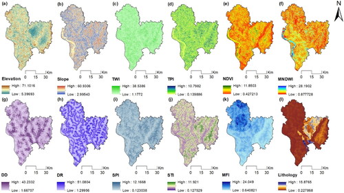
Table 14. Descriptive Statistics of single parameter sensitivity analysis of flood susceptibility.

Thematic Layers	Empirical Weight (%)	Effective Weight in %
		Min	Max	Mean	SD
Elevation	27%	5.40	71.10	29.26	9.17
Slope	19%	3.00	60.93	23.05	9.50
TWI	9%	1.18	38.54	5.56	3.50
TPI	2%	0.14	10.80	1.61	1.33
NDVI	3%	0.43	11.85	2.27	1.19
MNDWI	6%	0.88	28.19	4.16	2.37
Drainage Density (km/sq km)	12%	1.67	43.23	9.20	5.52
Distance from river (km)	12%	1.30	51.08	13.48	8.15
SPI	2%	0.12	12.17	2.66	1.53
STI	2%	0.13	11.92	3.59	1.46
MFI	4%	0.64	24.05	4.13	2.52
Lithology	3%	0.23	15.88	1.03	1.31

Similarly, when examining vulnerability, the two corresponding parameters, namely total population and population density, are assigned the highest empirical weight scores (23.5%). The sensitivity analysis and statistical findings for the FV zone reveal that out of the nine vulnerability conditioning parameters, the distance to the flood shelter has the highest mean effective weight score (19.96%), followed by LULC (18.27%). On the other hand, the employment rate has the lowest score (2.79%), which is succeeded by the illiteracy rate (4.90%). Among the parameters, the layer distance to the flood shelter (10.36%) exhibits the greatest disparity between the empirical and the mean effective weight scores (Table 15). The distance to the road, illiteracy, and employment rates exhibits relatively similar mean effective weight scores compared to the empirical weight scores (Figure 9).

Figure 9. Effective weight (W) for flood vulnerability parameters.

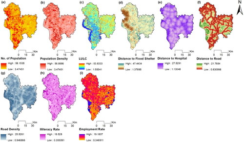
Table 15. Descriptive Statistics of single parameter sensitivity analysis of flood vulnerability.

Thematic Layers	Empirical Weight (%)	Effective Weight in %
		Min	Max	Mean	SD
Total Population	23.50	3.47	58.15	16.46	8.52
Population Density	23.50	3.47	56.89	16.71	8.08
LULC	15.30	1.50	53.83	18.27	7.99
Distance to Flood Shelter	9.60	1.38	47.44	19.96	6.58
Distance to Hospital	9.60	1.13	27.53	6.89	3.95
Distance to Road	6.00	0.83	21.77	5.64	4.50
Road Density	6.00	0.95	25.53	8.38	3.57
Illiteracy Rate	3.80	0.36	19.53	4.90	2.54
Employment Rate	2.70	0.35	19.18	2.79	1.58

4.4.3. Map removal sensitivity analysis

No significant variations were observed in the statistical output when conducting sensitivity analysis by removing individual parameters while considering all twelve susceptibility parameter layers. The highest variation in Sensitivity Index (SI) value (mean SI value variation = 1.16%) was observed upon removing the TWI layer, followed by the lithology layer (1.14%). Conversely, the lowest SI value (mean SI value variation = 0.72%) was observed in the STI layer, followed by the SPI layer (0.84%). The difference between the highest and lowest SI values is only 0.44%, suggesting that the chosen parameters do not significantly affect the FS map (Table 16). Figure 10 illustrates the Sensitivity Index values for FS parameters. Furthermore, the sensitivity analysis involved removing each thematic layer, and the percentage changes in the FSZwere examined. Figure 11 and Table 17 illustrate the map removal sensitivity analysis results, showing distinct variations in the percentage results of the FSZ maps. The highest increases in the percentage changes for the very low, low, moderate, high, and very high flood susceptible areas were observed when excluding the slope layer (+8.49%), MFI layer (−35.58%), elevation layer (+2.92%), distance from the river layer (+9.88%), and drainage density layer (+31.56%), respectively. Conversely, the highest decreases in the percentage changes for the very low, low, moderate, high, and very high flood-susceptible areas were observed upon removing the drainage density layer (−4.85%), drainage density layer (−10.29%), drainage density layer (−5.56%), MFI layer (+2.05), and slope layer (−1.34%), respectively.

Figure 10. Sensitivity index (SI) for flood susceptibility parameters.

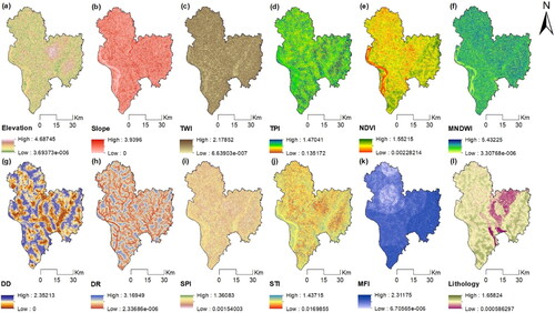
Figure 11. Flood susceptibility zonation with each parameter removal.

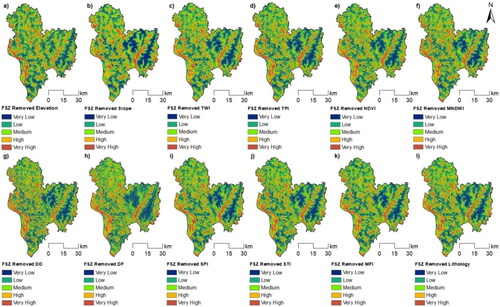
Table 16. Descriptive Statistics of map removal sensitivity analysis of flood susceptibility.

Thematic Layers	SI Variation in %
	Min	Max	Mean	SD
Elevation	3.7E-06	4.69	1.11	0.76
Slope	0.0E + 00	3.94	0.94	0.65
TWI	6.6E-07	2.18	1.16	0.35
TPI	1.4E-01	1.47	0.96	0.15
NDVI	2.3E-03	1.55	1.01	0.13
MNDWI	3.3E-06	5.43	1.06	0.37
Drainage Density (km/sq km)	0.0E + 00	2.35	1.12	0.47
Distance from river (km)	2.3E-06	3.17	0.86	0.51
SPI	1.5E-03	1.36	0.84	0.16
STI	1.7E-02	1.44	0.72	0.14
MFI	6.7E-06	2.31	0.99	0.28
Lithology	5.9E-04	1.66	1.13	0.13

Table 17. Percentage of changes of flood susceptibility zonation with the removal of each thematic layer.

Thematic Layer	FSZ (%)
	Very Low	Low	Medium	High	Very High
Elevation	+1.79	−7.98	+2.92	+3.14	+4.22
Slope	+8.49	−5.46	−4.46	+6.63	−1.34
TWI	−3.90	−5.47	+0.26	+4.97	+9.68
TPI	−0.60	−4.40	−0.61	+3.40	+6.99
NDVI	−1.73	−4.95	−0.76	+5.05	+7.40
MNDWI	−4.50	−7.27	−0.86	+6.27	+15.19
Drainage Density (km/sq km)	−4.85	−10.29	−5.56	+7.63	+31.56
Distance from river (km)	−2.11	−9.16	−1.66	+9.88	+11.49
SPI	−1.84	−5.39	−0.98	+4.88	+9.37
STI	−1.34	−5.21	−1.21	+4.84	+8.78
MFI	+3.13	−3.58	−0.37	+2.05	+1.03
Lithology	−0.94	−5.03	−0.58	+4.44	+7.00

‘+’ represents increased by area and ‘−‘represents decreased by area

The sensitivity analysis conducted on the vulnerability layers revealed that the thematic layer of population density exhibited the highest Sensitivity Index (SI) value (mean SI value variation = 2.99%), followed by the total population layer (2.80%). Conversely, the layer of distance to the flood shelter exhibited the lowest SI value (mean SI value variation = 0.68%), followed by the layer of road density (0.93%). The FVZ maps demonstrated relatively low sensitivity, with a difference of 2.31% between the highest and lowest SI values (Table 18). Figure 12 represents the Sensitivity Index values for the FV parameters. In terms of the percentage changes observed in the FV mapping through map removal sensitivity analysis, significant variations were observed when removing each thematic layer, as depicted in Figure 13 and Table 19. The highest increases in the percentage changes for the very low, low, moderate, high, and very high vulnerable areas were observed upon removing the distance to the flood shelter layer (+30.48%), distance to the road layer (+14.13%), total population layer (+25.67%), total population layer (+9.75%), and LULC layer (+23.54%), respectively. Conversely, the maximum decreases in the percentage changes of the FV zonation was observed by removing the total population layer (−37.25%), LULC layer (−4.25%), distance to flood shelter layer (−15.76%), road density layer (−12.00%), and population density layer (-26.17%), respectively.

Figure 12. Sensitivity index (SI) for flood vulnerability parameters.

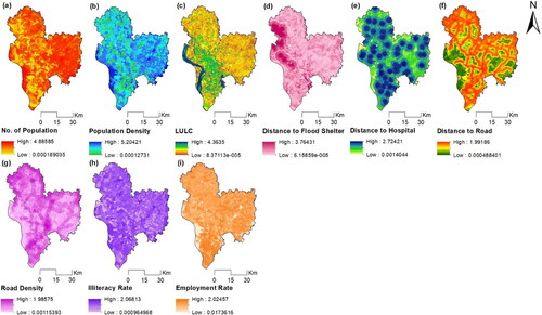
Figure 13. Flood vulnerability zonation with each parameter removal.

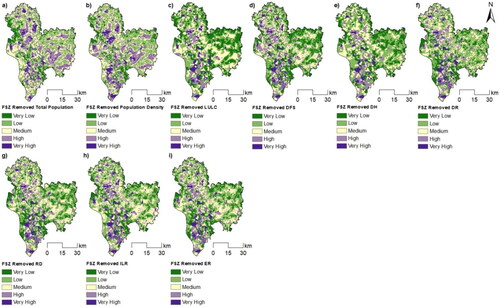
Table 18. Descriptive Statistics of map removal sensitivity analysis of flood vulnerability.

Thematic Layers	SI Variation in %
	Min	Max	Mean	SD
Total Population	1.9E-04	4.89	2.80	1.23
Population Density	1.3E-04	5.20	2.99	1.23
LULC	8.4E-05	4.36	1.34	0.87
Distance to Flood Shelter	6.2E-05	3.76	0.68	0.59
Distance to Hospital	1.4E-03	2.72	1.95	0.53
Distance to Road	4.9E-04	1.99	1.28	0.59
Road Density	1.2E-03	1.99	0.93	0.48
Illiteracy Rate	9.6E-04	2.07	1.32	0.34
Employment Rate	1.7E-02	2.02	1.58	0.24

Table 19. Percentage of changes of flood vulnerability zonation with removal of each thematic layer.

Thematic Layer	FVZ (%)
	Very Low	Low	Medium	High	Very High
Total Population	−37.25	−3.32	+25.67	+9.75	−17.26
Population Density	−28.03	+3.32	+20.91	−1.18	−26.17
LULC	+15.69	−4.28	−7.75	−4.88	+23.54
Distance to Flood Shelter	+30.48	+3.34	−15.76	−11.02	−1.74
Distance to Hospital	−12.43	+4.13	+2.19	+3.96	−7.12
Distance to Road	−11.96	+14.13	−3.42	−9.04	−2.38
Road Density	−0.18	+12.18	−4.20	−12.00	−11.93
Illiteracy Rate	+23.86	−0.89	−9.84	−7.05	+1.61
Employment Rate	−13.63	+0.53	+4.32	+2.99	+7.17

‘+’ represents increased by area and ‘- ‘represents decreased by area.

4.5. Validation of the model

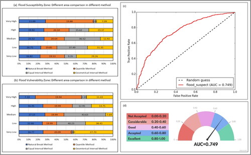
The ROC curve was used to validate the FS zonation map, as shown in Figure 14 (c, d). The task requires a flood inventory map. This study utilised geospatial data from BHUVAN a geo-platform developed by the ISRO (Indian Space Research Organisation), to identify historical flood and non-flood locations. The ROC curve depicts sensitivity pairs that correspond to distinct thresholds. This demonstrates the relationship between true and false positive rates for various cut-off values. The Area Under the Curve (AUC) is a quantitative metric used to evaluate the efficacy of a parameter in distinguishing between two diagnostic groups. An area under the curve (AUC) value ranging from 0.5 to 0.6 suggests a weakened level of predictive precision. The predictive accuracy of a model can be evaluated based on the area under the receiver operating characteristic curve (AUC). AUC values falling within the intervals of 0.6-0.7, 0.7-0.8, 0.8-0.9, and 0.9-1.0 indicate moderate, good, very good, and excellent prediction accuracy, respectively (Figure 14). Comprehending and precisely construing these metrics is crucial for proficiently evaluating the efficacy of diverse diagnostic modalities (Andualem and Demeke 2019; Mukherjee and Singh 2020; Mitra et al. 2022). The validation results indicate that the AHP approach revealed good prediction, as evidenced by the AUC of the FSZ map being 0.749 (74.90%).

Figure 14. (a) Classification of flood susceptibility zonation, (b) flood vulnerability zonation, (c) ROC-AUC analysis, (d) speedometer shows the AUC.

5. Discussion

This study effectively applies the Analytical Hierarchy Process (AHP) methodology to demarcate the FS zone (FSZ), FVZ, and flood risk zone (FRZ) in the flooded Malda District of West Bengal, India. The AHP is a statistical technique that utilizes expert knowledge and decision-making to effectively and consistently delineate the FRZ, making it a widely adopted method. This study seeks to suggest an alternative approach within this context.

This study aimed to determine the key factors contributing to FS and vulnerability assessment. It identified several indices, such as elevation, slope, drainage density, distance to the river, and TWI, which significantly influence FS. For vulnerability assessment, the researchers considered factors such as total population, population density, land use land cover (LULC), distance to flood shelter, and distance to the hospital. To assess flood intensity, the study incorporated various aspects, including geological, geomorphological, hydrological, meteorological, and environmental features. Demographic, social, economic, infrastructural, and land use patterns were also analyzed to evaluate vulnerability. Msabi and Makonyo (2021) showed that highly affected parameters for the identification of FS are elevation, slope, drainage density, LULC, soil type, geology, and flow accumulation. Souissi et al. (2019) showed that elevation, LULC, lithology, rainfall intensity (MFI), drainage density, distance to drainage network, slope, and groundwater depth are the most affected parameters for FS, about >72% weightage have been employed to the elevation, LULC, lithology, and rainfall intensity (MFI) layers. In the present study, 12 susceptibility and 9 vulnerability parameters have been chosen for the better identification of the risk region. Also done sensitivity analysis for the validation of the AHP model.

RS and GIS-based MCDM methods have been used to identify the model’s behaviour and limitations. However, MCDM rankings are usually uncertain due to raw data, data processing, criteria choice, and thresholds. The causes of the greatest controversy and ambiguity are often the criteria ratings or weights (Das and Gupta 2021; Mitra et al. 2022). To validate the weights assigned to AHP, three different types of sensitivity analyses are employed: Stillwell ranking method, single parameter sensitivity, and map removal sensitivity (Mukherjee and Singh 2020; Mitra et al. 2022). The cross-verification of the present study evaluates the ROC-AUC curve to investigate the reliability and efficiency of the AHP technique.

Flooding is a major cause of concern because of the damage it can do to properties, infrastructures, economic activities, and people’s livelihoods. There are several accepted methodologies for assessing susceptibility, vulnerability, and risk to flooding in this context. The fundamental goals of each of these methods are the same. To improve the accuracy with which this scenario is predicted. Although it is impossible to eliminate the risk of flooding, it may be mitigated by implementing the appropriate measures. In order to achieve this goal, it is crucial first to conduct a thorough investigation of any susceptible, vulnerable, or at-risk areas.

6. Conclusion

The MCDM AHP approach and its sensitivity analysis have been used to flood modeling in this study. When using the AHP to determine the viability and stability of a solution, a sensitivity analysis is a crucial step. It presents a means to investigate the matter of choice by examining the impact of alterations in criterion weights on spatial and quantitative assessment outcomes. Additionally, it facilitates quicker input for evaluators or modelers. GIS and MCDM would be better applied to real-world land-management difficulties if the discipline continued to develop in ways like sensitivity analysis on modifying criterion threshold levels, shifting the relative significance of criteria, etc. This study provides sensitivity analyses of the AHP technique, which can be used for data from anywhere in the world. This provides a precise representation of FS, vulnerability, and risk, enabling land-use planners and government authorities to implement measures to reduce risk effectively. The findings can provide valuable insights for land use planning before implementing flood management strategies in this region. Therefore, this research provides a unique perspective for studies that use several MCDM methods for modeling. Importantly, this study also identifies the region most in danger from flooding, which may aid the local executive in implementing a management and monitoring strategy for the affected district.

The area can only be improved by implementing an effective flood risk plan. Moreover, the areas most at threat are suggested to adopt flood protection (structural and non-structural) strategies. Implementing regulations to restrict residential development in flood-prone regions, enhancing the availability of flood shelters and healthcare facilities, adopting sustainable strategies for managing flood plains, acquiring flood insurance, and increasing public knowledge and understanding are all pivotal measures for mitigating flood hazards. Local governing bodies and emergency response teams can utilize the generated maps indicating susceptibility, vulnerability, and risk to assess the likelihood of flooding in various locations.

Since the MCDM method is used in the research, but it has some room for improvement, higher-resolution data and other methods more suited to the field might be used to make the necessary adjustments. Other sensitivity analyses might be used to evaluate the models in the study better. The main advantage of the method is the property given by the statement ‘depending on expert knowledge’. However, this is also the main disadvantage. Expert subjectivity, particularly in pairwise comparisons, constitutes the main drawback of the AHP. The utilization of machine learning techniques aids researchers in achieving a more profound understanding of flood-prone areas characterized by susceptibility, vulnerability, and risk. This enables them to conduct more precise assessments and evaluations in their study. The MCDM method has several limitations, but it may be useful for exploring genuine issues in places with little data, such as developing nations. Policymakers, government ministries and authorities, local administrative bodies, environmentalists, planners, and engineers may benefit from this research, and it has broad applicability because of the prevalence of floods globally.

Acknowledgement

This publication was financially supported by the Deanship of Scientific Research at the King Faisal University, Saudi Arabia (grant: 5,098).

Disclosure statement

No potential conflict of interest was reported by the author(s).

References

- Abdelkarim A, Al-Alola SS, Alogayell HM, Mohamed SA, Alkadi II, Ismail IY. 2020. Integration of GIS-based multicriteria decision analysis and analytic hierarchy process to assess flood hazard on the Al-Shamal Train pathway in Al-Qurayyat Region, Kingdom of Saudi Arabia. Water. 12(6):1702. doi: 10.3390/w12061702.
- Adiat K, Nawawi M, Abdullah K. 2012. Assessing the accuracy of GIS-based elementary multi criteria decision analysis as a spatial prediction tool – A case of predicting potential zones of sustainable groundwater resources. J Hydrol. 440-441:75–89. doi: 10.1016/j.jhydrol.2012.03.028.
- Agarwal R, Garg PK. 2015. Remote sensing and GIS based groundwater potential & recharge zones mapping using multi-criteria decision making technique. Water Resour Manage. 30(1):243–260. doi: 10.1007/s11269-015-1159-8.
- Ahmadlou M, Karimi M, Alizadeh S, Shirzadi A, Parvinnejhad D, Shahabi H, Panahi M. 2019. Flood susceptibility assessment using integration of adaptive network-based fuzzy inference system (ANFIS) and biogeography-based optimization (BBO) and BAT algorithms (BA). Geocarto Int. 34(11):1252–1272. doi: 10.1080/10106049.2018.1474276.
- Akay H. 2021. Flood hazards susceptibility mapping using statistical, fuzzy logic, and MCDM methods. Soft Comput. 25(14):9325–9346. doi: 10.1007/s00500-021-05903-1.
- Al-Aizari A, Al-Masnay YA, Aydda A, Zhang J, Ullah K, Islam ARMT, Habib T, Kaku DU, Nizeyimana JC, Al-Shaibah B, et al. 2022. Assessment analysis of flood susceptibility in tropical desert area: a case study of Yemen. Remote Sens. 14(16):4050. doi: 10.3390/rs14164050.
- Aldiansyah S, Wardani F. 2023. Evaluation of flood susceptibility prediction based on a resampling method using machine learning. J Water Clim Change. 14(3):937–961. doi: 10.2166/wcc.2023.494.
- Ali SA, Parvin F, Pham QB, Vojtek M, Vojteková J, Costache R, Linh NTT, Nguyen HQ, Ahmad A, Ghorbani MA. 2020. GIS-based comparative assessment of flood susceptibility mapping using hybrid multi-criteria decision-making approach, naïve Bayes tree, bivariate statistics and logistic regression: a case of Topľa basin, Slovakia. Ecol Indic. 117:106620. doi: 10.1016/j.ecolind.2020.106620.
- Andualem TG, Demeke GG. 2019. Groundwater potential assessment using GIS and remote sensing: a case study of Guna tana landscape, upper blue Nile Basin, Ethiopia. J Hydrol: Reg Stud. 24:100610. doi: 10.1016/j.ejrh.2019.100610.
- Annual Flood Report. 2019. West Bengal; [accessed 2022 Feb 20]. https://wbiwd.gov.in/uploads/annual_flood_report/ANNUAL_FLOOD_REPORT_2019.pdf.
- Auerbach LW, Goodbred SL, Mondal DR, Wilson C, Ahmed KR, Roy K, Steckler MS, Small C, Gilligan JM, Ackerly BA. 2015. Flood risk of natural and embanked landscapes on the Ganges–Brahmaputra tidal delta plain. Nat Clim Change. 5(2):153–157. doi: 10.1038/nclimate2472.
- Aydin HE, Iban MC. 2022. Predicting and analyzing flood susceptibility using boosting-based ensemble machine learning algorithms with SHapley Additive exPlanations. Nat Hazards. 116(3):2957–2991. doi: 10.1007/s11069-022-05793-y.
- Azareh A, Rafiei Sardooi E, Choubin B, Barkhori S, Shahdadi A, Adamowski J, Shamshirband S. 2019. Incorporating multi-criteria decision-making and fuzzy-value functions for flood susceptibility assessment. Geocarto Int. 36(20):2345–2365. doi: 10.1080/10106049.2019.1695958.
- Azizi M, Mohajerani A, Akhavan M. 2018. Simulating and prediction of flow using by WetSpa model in Ziyarat River Basin, Iran. OJG. 08(03):298–312. doi: 10.4236/ojg.2018.83019.
- Bahremand A, De Smedt F, Corluy J, Liu YW, Poorova J, Velcicka L, Kunikova E. 2007. WetSpa model application for assessing reforestation impacts on floods in Margecany–Hornad Watershed, Slovakia. Water Resour Manage. 21(8):1373–1391. doi: 10.1007/s11269-006-9089-0.
- Baig MA, Xiong D, Rahman M, Islam MM, Elbeltagi A, Yigez B, Rai DK, Tayab MR, Dewan A. 2021. How do multiple kernel functions in machine learning algorithms improve precision in flood probability mapping? Nat Hazards. 113: 1543–1562. doi: 10.21203/rs.3.rs-749595/v1.
- Balamurugan R, Choudhary K, Raja SP. 2022. Prediction of flooding due to heavy rainfall in India using machine learning algorithms: providing advanced warning. IEEE Syst Man Cybern Mag. 8(4):26–33. doi: 10.1109/MSMC.2022.3183806.
- Bera S, Das A, Mazumder T. 2022. Evaluation of machine learning, information theory and multi-criteria decision analysis methods for flood susceptibility mapping under varying spatial scale of analyses. Remote Sens Appl: Soc Environ. 25:100686. doi: 10.1016/j.rsase.2021.100686.
- Beven KJ, Kirkby MJ. 1979. A physically based, variable contributing area model of basin hydrology/Un modèle à base physique de zone d’appel variable de l’hydrologie du bassin versant. Hydrol Sci Bull. 24(1):43–69. doi: 10.1080/02626667909491834.
- Bhardwaj S, Veerappan R. 2023. Flood susceptibility zonation using Dempster-Shafer evidential belief function (EBF) method in Chalakudy Taluk, Kerala, India. Switzerland AG: Springer eBooks; p. 79–109. doi: 10.1007/978-3-031-21618-3_5.
- Bhattacharjee S, Kumar P, Thakur PK, Gupta K. 2020. Hydrodynamic modelling and vulnerability analysis to assess flood risk in a dense Indian city using geospatial techniques. Nat Hazards. 105(2):2117–2145. doi: 10.1007/s11069-020-04392-z.
- Biswas S, Mitra R, Roy D, Mandal DK. 2022. Flash flood susceptibility mapping in Alipurduar district using multi-criteria decision analysis approach. Res Square. doi: 10.21203/rs.3.rs-2093997/v1.
- Bouamrane A, Derdous O, Dahri N, Tachi SE, Boutebba K, Bouziane MT. 2020. A comparison of the analytical hierarchy process and the fuzzy logic approach for flood susceptibility mapping in a semi-arid ungauged basin (Biskra basin: Algeria). Int J River Basin Manage. 20(2):203–213. doi: 10.1080/15715124.2020.1830786.
- Bui DT, Arabameri A, Islam ARMT, Abba SI, Pandey MK, Ajin RS, Pham BT. 2022. Flood susceptibility computation using state-of-the-art machine learning and optimization algorithms. Res Square. doi: 10.21203/rs.3.rs-1405369/v1.
- Bui DT, Khosravi K, Shahabi H, Daggupati P, Adamowski J, Melesse AM, Pham BT, Pourghasemi HR, Mahmoudi M, Bahrami S, et al. 2019. Flood spatial modeling in Northern Iran using remote sensing and GIS: a comparison between evidential belief functions and its ensemble with a multivariate logistic regression model. Remote Sensing. 11(13):1589. doi: 10.3390/rs11131589.
- Cabrera JS, Lee HS. 2020. Flood risk assessment for Davao Oriental in the Philippines using geographic information system‐based multi‐criteria analysis and the maximum entropy model. J Flood Risk Manage. 13(2):e12607. doi: 10.1111/jfr3.12607.
- Cao Y, Jia H, Xiong J, Cheng W, Li K, Pang Q, Yong Z. 2020. Flash flood susceptibility assessment based on geodetector, certainty factor, and logistic regression analyses in Fujian Province, China. IJGI. 9(12):748. doi: 10.3390/ijgi9120748.
- Central Water Commission, Annual Report 2009–10. 2010. Ministry of Water Resources, Government of India; [accessed 2022 Feb 20]. https://cwc.gov.in/sites/default/files/Final%20Annual%20Report%202009_10.pdf.
- Chakraborty S, Mukhopadhyay S. 2019. Assessing flood risk using analytical hierarchy process (AHP) and geographical information system (GIS): application in Coochbehar district of West Bengal, India. Nat Hazards. 99(1):247–274. doi: 10.1007/s11069-019-03737-7.
- Chang DY. 1996. Applications of the extent analysis method on fuzzy AHP. Eur J Oper Res. 95(3):649–655. doi: 10.1016/0377-2217(95)00300-2.
- Chattaraj D, Paul B, Sarkar S. 2021. Integrated multi-parametric analytic hierarchy process (AHP) and geographic information system (GIS) based spatial modelling for flood and water logging susceptibility mapping: a case study of English Bazar Municipality of Malda, West Bengal, India. Nat Hazards Earth Syst Sci Discuss. :1–20. doi: 10.5194/nhess-2020-399.
- Chen TY. 2021. A likelihood-based preference ranking organization method using dual point operators for multiple criteria decision analysis in Pythagorean fuzzy uncertain contexts. Expert Syst Appl. 176:114881. doi: 10.1016/j.eswa.2021.114881.
- Chen W, Hong H, Li S, Shahabi H, Wang Y, Wang X, Ahmad BB. 2019. Flood susceptibility modelling using novel hybrid approach of reduced-error pruning trees with bagging and random subspace ensembles. J Hydrol. 575:864–873. doi: 10.1016/j.jhydrol.2019.05.089.
- Chen G, Hou J, Zhou N, Yang S, Tong Y, Su F, Huang L, Bi X. 2020. High-resolution urban flood forecasting by using a coupled atmospheric and hydrodynamic flood models. Front Earth Sci. 8:545612. doi: 10.3389/feart.2020.545612.
- Chenini I, Ben Mammou A. 2010. Groundwater recharge study in arid region: An approach using GIS techniques and numerical modeling. Comput Geosci. 36(6):801–817. doi: 10.1016/j.cageo.2009.06.014.
- Chen W, Li Y, Xue W, Shahabi H, Li S, Hong H, Wang X, Bian H, Zhang S, Pradhan B, et al. 2020. Modeling flood susceptibility using data-driven approaches of naïve Bayes tree, alternating decision tree, and random forest methods. Sci Total Environ. 701:134979. doi: 10.1016/j.scitotenv.2019.134979.
- Chiu Y, Raina N, Chen H. 2021. Evolution of flood defense strategies: toward nature-based solutions. Environments. 9(1):2. doi: 10.3390/environments9010002.
- Chowdhuri I, Pal SC, Chakrabortty R. 2020. Flood susceptibility mapping by ensemble evidential belief function and binomial logistic regression model on river basin of eastern India. Adv Space Res. 65(5):1466–1489. doi: 10.1016/j.asr.2019.12.003.
- Costache R, Trung Tin T, Arabameri A, Crăciun A, Ajin RS, Costache I, Reza Md. Towfiqul Islam A, Abba SI, Sahana M, Avand M, et al. 2022. Flash-flood hazard using deep learning based on H2O R package and fuzzy-multicriteria decision-making analysis. J Hydrol. 609:127747. doi: 10.1016/j.jhydrol.2022.127747.
- Costache R. 2019. Flood susceptibility assessment by using bivariate statistics and machine learning models - a useful tool for flood risk management. Water Resour Manage. 33(9):3239–3256. doi: 10.1007/s11269-019-02301-z.
- Costache R, Arabameri A, Costache I, Crăciun AM, Pham BT. 2022. New machine learning ensemble for flood susceptibility estimation. Water Resour Manage. 36(12):4765–4783. doi: 10.1007/s11269-022-03276-0.
- Costache R, Barbulescu A, Pham Q. 2021. Integrated framework for detecting the areas prone to flooding generated by flash-floods in small river catchments. Water. 13(6):758. doi: 10.3390/w13060758.
- Costache R, Ngo PTT, Bui DT. 2020. Novel ensembles of deep learning neural network and statistical learning for flash-flood susceptibility mapping. Water. 12(6):1549. doi: 10.3390/w12061549.
- Costache R, Pham QB, Arabameri A, Diaconu DC, Costache I, Crăciun A, Ciobotaru N, Pandey M, Arora A, Ali SA, et al. 2021. Flash-flood propagation susceptibility estimation using weights of evidence and their novel ensembles with multicriteria decision making and machine learning. Geocarto Int. 37(25):8361–8393. doi: 10.1080/10106049.2021.2001580.
- Da Silva L, Alencar MS, De Almeida AT. 2020. Multidimensional flood risk management under climate changes: bibliometric analysis, trends and strategic guidelines for decision-making in urban dynamics. Int J Disaster Risk Reduct. 50:101865. doi: 10.1016/j.ijdrr.2020.101865.
- Danumah JH, Odai SN, Saley B, Szarzynski J, Thiel MA, Kwaku AA, Kouame FK, Akpa LY. 2016. Flood risk assessment and mapping in Abidjan district using multi-criteria analysis (AHP) model and geoinformation techniques, (Cote d’ivoire). Geoenviron Disasters. 3(1):1–13. doi: 10.1186/s40677-016-0044-y.
- Das S. 2018. Geographic information system and AHP-based flood hazard zonation of Vaitarna basin, Maharashtra, India. Arab J Geosci. 11:576. doi: 10.1007/s12517-018-3933-4.
- Das S. 2020. Flood susceptibility mapping of the Western Ghat coastal belt using multi-source geospatial data and analytical hierarchy process (AHP). Remote Sens Appl: Soc Environ. 20:100379. doi: 10.1016/j.rsase.2020.100379.
- Das S, Gupta A. 2021. Multi-criteria decision based geospatial mapping of flood susceptibility and temporal hydro-geomorphic changes in the Subarnarekha basin, India. Geosci Front. 12(5):101206. doi: 10.1016/j.gsf.2021.101206.
- Das S, Gupta A, Ghosh S. 2017. Exploring groundwater potential zones using MIF technique in semi-arid region: a case study of Hingoli district, Maharashtra. Spat Inf Res. 25(6):749–756. doi: 10.1007/s41324-017-0144-0.
- Das B, Mondal M, Das A. 2012. Monitoring of bank line erosion of River Ganga, Malda District, and West Bengal: using RS and GIS compiled with statistical techniques. Int J Geomat Geosci. 3(1):239–248.
- Das S, Pal S. 2016. Character and cardinality of channel migration of Kalindri River, West Bengal, India. Int Res J Earth Sci. 4(1):13–26.
- Das S, Pardeshi SD. 2017. Comparative analysis of lineaments extracted from Cartosat, SRTM and ASTER DEM: a study based on four watersheds in Konkan region, India. Spat Inf Res. 26(1):47–57. doi: 10.1007/s41324-017-0155-x.
- Das S, Pardeshi SD. 2018. Integration of different influencing factors in GIS to delineate groundwater potential areas using IF and FR techniques: a study of Pravara basin, Maharashtra, India. Appl Water Sci. 8(7):197. doi: 10.1007/s13201-018-0848-x.
- Das S, Pardeshi SD. 2018. Morphometric analysis of Vaitarna and Ulhas river basins, Maharashtra, India: using geospatial techniques. Appl Water Sci. 8:158. doi: 10.1007/s13201-018-0801-z.
- Das S, Pardeshi SD, Kulkarni PP, Doke A. 2018. Extraction of lineaments from different azimuth angles using geospatial techniques: a case study of Pravara basin, Maharashtra, India. Arab J Geosci. 11:1–13. doi: 10.1007/s12517-018-3522-6.
- Das S, Scaringi G. 2021. River flooding in a changing climate: rainfall-discharge trends, controlling factors, and susceptibility mapping for the Mahi catchment, Western India. Nat Hazards. 109(3):2439–2459. doi: 10.1007/s11069-021-04927-y.
- De Reu J, Bourgeois J, Bats M, Zwertvaegher A, Gelorini V, De Smedt P, Chu W, Antrop M, De Maeyer P, Finke P, et al. 2013. Application of the topographic position index to heterogeneous landscapes. Geomorphology. 186:39–49. doi: 10.1016/j.geomorph.2012.12.015.
- Dhar O, Nandargi S. 2003. Hydrometeorological aspects of floods in India. Nat Hazards. 28(1):1–33. doi: 10.1023/A:1021199714487.
- Di Baldassarre G, Montanari A, Lins HF, Koutsoyiannis D, Brandimarte L, Blöschl G. 2010. Flood fatalities in Africa: from diagnosis to mitigation. Geophys Res Lett. 37(22):L22402. doi: 10.1029/2010GL045467.
- Disaster Management Department, Government of West Bengal. 2018. District disaster management plan of Malda. WBDMD; [accessed 2019]. http://wbdmd.gov.in/Pages/District_DM_Plan.aspx.
- Disaster Management Department, Government of West Bengal. 2016. District disaster management plan of Malda. WBDMD; [accessed 2017 Sep 1]. http://wbdmd.gov.in/Pages/District_DM_Plan.aspx.
- Disaster Management Department, Government of West Bengal. 2019–2020. District disaster management plan of Maldah. WBDMD; [accessed 2020 Feb]. http://wbdmd.gov.in/Pages/District_DM_Plan.aspx.
- District Census Handbook of Maldah District (DCHM), Census of India. 2011. West Bengal. https://www.censusindia.gov.in/2011census/dchb/WB.html.
- Duan Y, Meng F, Liu T, Huang Y, Luo M, Xing W, De Maeyer P. 2019. Sub-daily simulation of mountain flood processes based on the modified soil water assessment tool (SWAT) model. IJERPH. 16(17):3118. doi: 10.3390/ijerph16173118.
- Edamo ML, Ukumo TY, Lohani TK, Ayana MT, Ayele MA, Mada ZM, Abdi DM. 2022. A comparative assessment of multi-criteria decision-making analysis and machine learning methods for flood susceptibility mapping and socio-economic impacts on flood risk in Abela-Abaya floodplain of Ethiopia. Environ Chall. 9:100629. doi: 10.1016/j.envc.2022.100629.
- Edet A, Okereke C. 1997. Assessment of hydrogeological conditions in basement aquifers of the Precambrian Oban massif, southeastern Nigeria. J Appl Geophys. 36(4):195–204. doi: 10.1016/s0926-9851(96)00049-3.
- Eingrüber N, Korres W. 2022. Climate change simulation and trend analysis of extreme precipitation and floods in the mesoscale Rur catchment in western Germany until 2099 using Statistical Downscaling Model (SDSM) and the Soil & Water Assessment Tool (SWAT model). Sci Total Environ. 838(Pt 1):155775. doi: 10.1016/j.scitotenv.2022.155775.
- Elewa HH, Qaddah AA. 2011. Groundwater potentiality mapping in the Sinai Peninsula, Egypt, using remote sensing and GIS-watershed-based modelling. Hydrogeol J. 19(3):613–628. doi: 10.1007/s10040-011-0703-8.
- Elong A, Zhou L, Karney BW, Fang H, Cao Y, Assam SLZ. 2022. Flood prediction with two-dimensional shallow water equations: a case study of Tongo-Bassa Watershed in Cameroon. Appl Sci. 12(22):11622. doi: 10.3390/app122211622.
- Feby B, Achu AL, Jimnisha K, Ayisha VA, Reghunath R. 2020. Landslide susceptibility modelling using integrated evidential belief function based logistic regression method: a study from Southern Western Ghats, India. Remote Sens Appl: Soc Environ. 20:100411. doi: 10.1016/j.rsase.2020.100411.
- Gauhar N, Das S, Moury K. 2021. Prediction of flood in Bangladesh using k-nearest neighbors algorithm. 2021 2nd International Conference on Robotics, Electrical and Signal Processing Techniques (ICREST). doi: 10.1109/ICREST51555.2021.9331199.
- Fenta AA, Kifle A, Gebreyohannes T, Hailu G. 2014. Spatial analysis of groundwater potential using remote sensing and GIS-based multi-criteria evaluation in Raya Valley, northern Ethiopia. Hydrogeol J. 23(1):195–206. doi: 10.1007/s10040-014-1198-x.
- Getahun GY, Gebre SL. 2015. Flood hazard assessment and mapping of flood inundation area of the Awash River Basin in Ethiopia using GIS and HEC-GeoRAS/HEC-RAS model. J Civ Environ Eng. 05(04):1–12. doi: 10.4172/2165-784x.1000179.
- Ghorabaee MK, Amiri M, Zavadskas EK, Turskis Z. 2017. Multi-criteria group decision-making using an extended edas method with interval type-2 fuzzy sets. E + M. 20(1):48–68. doi: 10.15240/tul/001/2017-1-004.
- Ghosh A, Kar SK. 2018. Application of analytical hierarchy process (AHP) for flood risk assessment: a case study in Malda district of West Bengal, India. Nat Hazards. 94(1):349–368. doi: 10.1007/s11069-018-3392-y.
- Ghosh S, Saha S, Bera B. 2022. Flood susceptibility zonation using advanced ensemble machine learning models within Himalayan foreland basin. Nat Hazards Res. 2(4):363–374. doi: 10.1016/j.nhres.2022.06.003.
- Gigović L, Pamučar D, Bajić Z, Drobnjak S. 2017. Application of GIS-interval rough AHP methodology for flood hazard mapping in urban areas. Water. 9(6):360. doi: 10.3390/w9060360.
- Golkarian A, Naghibi SA, Kalantar B, Pradhan B. 2018. Groundwater potential mapping using C5.0, random forest, and multivariate adaptive regression spline models in GIS. Environ Monit Assess. 190:1–16. doi: 10.1007/s10661-018-6507-8.
- Grillakis MG, Tsanis IK, Koutroulis AG. 2010. Application of the HBV hydrological model in a flash flood case in Slovenia. Nat Hazards Earth Syst Sci. 10(12):2713–2725. doi: 10.5194/nhess-10-2713-2010.
- Habibi A, Delavar MR, Sadeghian MS, Nazari B. 2023. Flood susceptibility mapping and assessment using regularized random forest and Naïve Bayes algorithms. ISPRS Ann Photogramm Remote Sens Spatial Inf Sci. X-4/W1-2022:241–248. doi: 10.5194/isprs-annals-X-4-W1-2022-241-2023.
- Hammami S, Zouhri L, Souissi D, Souei A, Zghibi A, Marzougui A, Dlala M. 2019. Application of the GIS based multi-criteria decision analysis and analytical hierarchy process (AHP) in the flood susceptibility mapping (Tunisia). Arab J Geosci. 12:1–16. doi: 10.1007/s12517-019-4754-9.
- Hanley JA, McNeil BJ. 1982. The meaning and use of the area under a receiver operating characteristic (ROC) curve. Radiology. 143(1):29–36. doi: 10.1148/radiology.143.1.7063747.
- Hasanloo M, Pahlavani P, Bigdeli B. 2019. Flood risk zonation using a multi-criteria spatial group fuzzy-AHP decision making and fuzzy overlay analysis. Int Arch Photogramm Remote Sens Spatial Inf Sci. XLII-4/W18:455–460. doi: 10.5194/isprs-archives-XLII-4-W18-455-2019.
- Hasanuzzaman M, Adhikary PP, Bera B, Shit PK. 2022. Flood vulnerability assessment using AHP and frequency ratio techniques. In: Pradhan B, Shit PK, Bhunia GS, Adhikary PP, Pourghasemi HR, editors. Spatial modelling of flood risk and flood hazards. GIScience and geo-environmental modelling. Cham: Springer EBooks; p. 91–104. doi: 10.1007/978-3-030-94544-2_6.
- Hasanuzzaman M, Islam A, Bera B, Shit PK. 2022. A comparison of performance measures of three machine learning algorithms for flood susceptibility mapping of river Silabati (tropical river, India). Phys Chem Earth Parts a/B/C. 127:103198. doi: 10.1016/j.pce.2022.103198.
- Hasanuzzaman M, Shit PK, Bera B, Islam A. 2023. Characterizing recurrent flood hazards in the Himalayan foothill region through data-driven modelling. Adv Space Res. 71(12):5311–5326. doi: 10.1016/j.asr.2023.02.028.
- Hemmati M, Ellingwood BR, Mahmoud H. 2020. The role of urban growth in resilience of communities under flood risk. Earth’s Future. 8(3):e2019EF001382. doi: 10.1029/2019ef001382.
- Hidayah E, Halik G, Indarto I, Khaulan DW. 2022. Flood hazard mapping of the Welang river, Pasuruan, East Java, Indonesia. J Appl Water Eng Res. 11(3):333–344. doi: 10.1080/23249676.2022.2114025.
- Hidayah E, Halik G, Widiarti WY. 2022. Assessment of the conditioning factor for flash flood susceptibility potential based on bivariate statistical approach in the Wonoboyo Watershed in East Java. Indonesia. In Proceedings of the 5th International Conference on Rehabilitation and Maintenance in Civil Engineering ; pp. 553 – 573). doi: 10.1007/978-981-16-9348-9_49.
- Hidayah, E., Indarto, I., Lee, W., Halik, G., & Pradhan, B. (2022). Assessing coastal flood susceptibility in East Java, Indonesia: comparison of statistical bivariate and machine learning techniques. Water, 14(23), 3869. doi: 10.3390/w14233869.
- Hidayah E, Widiarti WY, Putra PP, Dewantie AA, Alhamda MZ, Prastika H. 2021. Evaluation of hydrologic modelling using satellite product, and MMR rainfall in East Java, Indonesia. J Ecol Eng. 22(11):246–260. doi: 10.12911/22998993/142843.
- Hoque M, Tasfia S, Ahmed N, Pradhan B. 2019. Assessing spatial flood vulnerability at Kalapara Upazila in Bangladesh using an analytic hierarchy process. Sensors (Basel). 19(6):1302. doi: 10.3390/s19061302.
- Horton RE. 1932. Drainage basin characteristics. Trans Am Geophys Union. 14:350–361. doi: 10.1029/TR013i001p00350.
- Huang W, Cao Z, Huang M, Duan W, Ni Y, Yang W. 2019. A new flash flood warning scheme based on hydrodynamic modelling. Water. 11(6):1221. doi: 10.3390/w11061221.
- Hussain M, Tayyab M, Ullah K, Ullah S, Rahman ZU, Zhang J, Al-Shaibah B. 2023. Development of a new integrated flood resilience model using machine learning with GIS-based multi-criteria decision analysis. Urban Clim. 50:101589. doi: 10.1016/j.uclim.2023.101589.
- Islam MR, Raja DR. 2021. Waterlogging risk assessment: an undervalued disaster risk in coastal urban community of Chattogram, Bangladesh. Earth. 2(1):151–173. doi: 10.3390/earth2010010.
- Jahangir MH, Reineh SMM, Abolghasemi M. 2019. Spatial predication of flood zonation mapping in Kan River Basin, Iran, using artificial neural network algorithm. Weather Clim Extremes. 25:100215. doi: 10.1016/j.wace.2019.100215.
- Jasrotia AS, Kumar R, Saraf AK. 2007. Delineation of groundwater recharge sites using integrated remote sensing and GIS in Jammu district, India. Int J Remote Sens. 28(22):5019–5036. doi: 10.1080/01431160701264276.
- Jenifer MA, Jha MK. 2017. Comparison of analytic hierarchy process, catastrophe and entropy techniques for evaluating groundwater prospect of hard-rock aquifer systems. J Hydrol. 548:605–624. doi: 10.1016/j.jhydrol.2017.03.023.
- Jenness J, Brost B, Beier P. 2013. Land facet corridor designer. USDA Forest Service Rocky Mountain Research Station, 1–110. https://corridordesign.org.
- Jesna I, Bhallamudi SM, Sudheer KP. 2023. Impact of cross‐sectional orientation in one‐dimensional hydrodynamic modeling on flood inundation mapping. J Flood Risk Manage. 16(3):e12893. doi: 10.1111/jfr3.12893.
- Jha MK, Chowdary VM, Chowdhury A. 2010. Groundwater assessment in Salboni Block, West Bengal (India) using remote sensing, geographical information system and multi-criteria decision analysis techniques. Hydrogeol J. 18(7):1713–1728. doi: 10.1007/s10040-010-0631-z.
- Kafle MR, Shakya NM. 2018. Multi-criteria decision making approach for flood risk and sediment management in Koshi Alluvial Fan, Nepal. JWARP. 10(06):596–619. doi: 10.4236/jwarp.2018.106034.
- Karande P, Chakraborty S. 2012. Application of multi-objective optimization on the basis of ratio analysis (MOORA) method for materials selection. Mater Des. 37:317–324. doi: 10.1016/j.matdes.2012.01.013.
- Kazakis N, Kougias I, Patsialis T. 2015. Assessment of flood hazard areas at a regional scale using an index-based approach and analytical hierarchy process: application in Rhodope–Evros region, Greece. Sci Total Environ. 538:555–563. doi: 10.1016/j.scitotenv.2015.08.055.
- Keshavarz Ghorabaee M, Amiri M, Zavadskas EK, Turskis Z, Antucheviciene J. 2017. A new multi-criteria model based on interval type-2 fuzzy sets and EDAS method for supplier evaluation and order allocation with environmental considerations. Comput Ind Eng. 112:156–174. doi: 10.1016/j.cie.2017.08.017.
- Khiavi AN, Vafakhah M, Sadeghi SH. 2023. Flood-based critical sub-watershed mapping: comparative application of multi-criteria decision making methods and hydrological modeling approach. Stoch Environ Res Risk Assess. 37(7):2757–2775. doi: 10.1007/s00477-023-02417-0.
- Kohansarbaz A, Kohansarbaz A, Shabanlou S, Yosefvand F, Rajabi A. 2022. Modelling flood susceptibility in northern Iran: application of five well‐known machine‐learning models. Irrig Drain. 71(5):1332–1350. doi: 10.1002/ird.2745.
- Kourgialas NN, Karatzas GP. 2011. Flood management and a GIS modelling method to assess flood-hazard areas—a case study. Hydrol Sci J. 56(2):212–225. doi: 10.1080/02626667.2011.555836.
- Kulkarni N, Shete VV. 2014. Hybrid neuro-fuzzy approach for flood prediction and Dam gate control. International Conference on Information Society. doi: 10.1109/i-society.2014.7009044.
- Kumar N, Liu XL, Narayanasamydamodaran S, Pandey KK. 2021. A Systematic review comparing urban flood management practices in India to China’s Sponge City program. Sustainability. 13(11):6346. doi: 10.3390/su13116346.
- Lee S, Kim JC, Jung HS, Lee MJ, Lee S. 2017. Spatial prediction of flood susceptibility using random-forest and boosted-tree models in Seoul metropolitan city, Korea. Geomat Nat Hazards Risk. 8(2):1185–1203. doi: 10.1080/19475705.2017.1308971.
- Liu YW, De Smedt F. 2005. Flood modeling for complex terrain using GIS and remote sensed information. Water Resour Manage. 19(5):605–624. doi: 10.1007/s11269-005-6808-x.
- Liu J, Shao W, Xiang C, Mei C, Li Z. 2020. Uncertainties of urban flood modeling: influence of parameters for different underlying surfaces. Environ Res. 182:108929. doi: 10.1016/j.envres.2019.108929.
- Lodwick WA, Monson W, Svoboda L. 1990. Attribute error and sensitivity analysis of map operations in geographical informations systems: suitability analysis. Int J Geogr Inf Syst. 4(4):413–428. doi: 10.1080/02693799008941556.
- Magesh N, Chandrasekar N, Soundranayagam JP. 2012. Delineation of groundwater potential zones in Theni district, Tamil Nadu, using remote sensing, GIS and MIF techniques. Geosci Front. 3(2):189–196. doi: 10.1016/j.gsf.2011.10.007.
- Mahmoud SH, Gan TY. 2018. Multi-criteria approach to develop flood susceptibility maps in arid regions of Middle East. J Cleaner Prod. 196:216–229. doi: 10.1016/j.jclepro.2018.06.047.
- Mahmoud SH, Gan TY. 2018. Urbanization and climate change implications in flood risk management: developing an efficient decision support system for flood susceptibility mapping. Sci Total Environ. 636:152–167. doi: 10.1016/j.scitotenv.2018.04.282.
- Maiti PK, Mandal S. 2019. Majority of actinobacterial strains isolated from Kashmir Himalaya soil are rich source of antimicrobials and industrially important biomolecules. AiM. 09(03):220–238. doi: 10.4236/aim.2019.93016.
- Maity DK, Mandal S. 2017. Identification of groundwater potential zones of the Kumari river basin, India: an RS & GIS based semi-quantitative approach. Environ Dev Sustain. 21(2):1013–1034. doi: 10.1007/s10668-017-0072-0.
- Malik S, Pal SC, Chowdhuri I, Chakrabortty R, Roy P, Das B. 2020. Prediction of highly flood prone areas by GIS based heuristic and statistical model in a monsoon dominated region of Bengal Basin. Remote Sens Appl: Soc Environ. 19:100343. doi: 10.1016/j.rsase.2020.100343.
- Mehebub S, Raihan A, Nuhul H, Haroon S. 2015. Assessing flood inundation extent and landscape vulnerability to flood using geospatial technology: A study of Malda district of West Bengal, India. fg. XIV(2):156–163. doi: 10.5775/fg.2067-4635.2015.144.d.
- Meyer V, Kuhlicke C, Luther J, Fuchs S, Priest SJ, Dorner W, Serrhini K, Pardoe J, McCarthy S, Seidel J, et al. 2012. Recommendations for the user-specific enhancement of flood maps. Nat Hazards Earth Syst Sci. 12(5):1701–1716. doi: 10.5194/nhess-12-1701-2012.
- Miller AJ. 1990. Flood hydrology and geomorphic effectiveness in the central Appalachians. Earth Surf Processes Landf. 15(2):119–134. doi: 10.1002/esp.3290150203.
- Ministry Home Affairs, Annual Report 2019-20. 2020. Ministry of Home Affairs, Government Of India; [accessed 2022 Feb 20]. https://www.mha.gov.in/sites/default/files/AnnualReport_19_20.pdf.
- Ministry Home Affairs, Annual Report 2021-22. 2022. Ministry of Home Affairs, Government Of India; [accessed 2022 Feb 20]. https://www.mha.gov.in/sites/default/files/AnnualReport202122_24112022%5B1%5D.pdf.
- Mishra K, Sinha R. 2020. Flood risk assessment in the Kosi megafan using multi-criteria decision analysis: a hydro-geomorphic approach. Geomorphology. 350:106861. doi: 10.1016/j.geomorph.2019.106861.
- Mitra R, Das J. 2022. A comparative assessment of flood susceptibility modelling of GIS-based TOPSIS, VIKOR and EDAS techniques in the Sub-Himalayan foothills region of Eastern India. Environ Sci Pollut Res. 30:16036–16067. doi: 10.21203/rs.3.rs-1710264/v1.
- Mitra RK, Saha P, Das J. 2022. Assessment of the performance of GIS-based analytical hierarchical process (AHP) approach for flood modelling in Uttar Dinajpur district of West Bengal, India. Geomat Nat Hazards Risk. 13(1):2183–2226. doi: 10.1080/19475705.2022.2112094.
- Moayedi H, Canatalay PJ, Dehrashid AA, Cifci MA, Salari M, Le BN. 2023. Multilayer perceptron and their comparison with two nature-inspired hybrid techniques of biogeography-based optimization (BBO) and backtracking search algorithm (BSA) for assessment of landslide susceptibility. Land. 12(1):242. doi: 10.3390/land12010242.
- Mojaddadi H, Pradhan B, Nampak H, Ahmad N, Ghazali AHB. 2017. Ensemble machine-learning-based geospatial approach for flood risk assessment using multi-sensor remote-sensing data and GIS. Geomat Nat Hazards Risk. 8(2):1080–1102. doi: 10.1080/19475705.2017.1294113.
- Mondal K, Bandyopadhyay S, Karmakar S. 2023. Framework for global sensitivity analysis in a complex 1D-2D coupled hydrodynamic model: highlighting its importance on flood management over large data-scarce regions. J Environ Manage. 332:117312. doi: 10.1016/j.jenvman.2023.117312.
- Mondal NC, Das SN, Singh VS. 2008. Integrated approach for identification of potential groundwater zones in Seethanagaram Mandal of Vizianagaram District, Andhra Pradesh, India. J Earth Syst Sci. 117(2):133–144. doi: 10.1007/s12040-008-0004-3.
- Moore ID, Hutchinson MF. 1990. Spatial extension of hydrologic process modelling.
- Mosavi A, Ozturk P, Chau KW. 2018. Flood prediction using machine learning models: literature review. Water. 10(11):1536. doi: 10.3390/w10111536.
- Msabi MM, Makonyo M. 2021. Flood susceptibility mapping using GIS and multi-criteria decision analysis: a case of Dodoma region, central Tanzania. Remote Sens Appl: Soc Environ. 21:100445. doi: 10.1016/j.rsase.2020.100445.
- Mukherjee K, Pal S. 2017. Channel migration zone mapping of the River Ganga in the Diara surrounding region of Eastern India. Environ Dev Sustain. 20(5):2181–2203. doi: 10.1007/s10668-017-9984-y.
- Mukherjee I, Singh UK. 2020. Delineation of groundwater potential zones in a drought-prone semi-arid region of east India using GIS and analytical hierarchical process techniques. Catena. 194:104681. doi: 10.1016/j.catena.2020.104681.
- Muralitharan J, Palanivel K. 2015. Groundwater targeting using remote sensing, geographical information system and analytical hierarchy process method in hard rock aquifer system, Karur district, Tamil Nadu, India. Earth Sci Inform. 8(4):827–842. doi: 10.1007/s12145-015-0213-7.
- Naghibi SA, Pourghasemi HR, Abbaspour K. 2017. A comparison between ten advanced and soft computing models for groundwater qanat potential assessment in Iran using R and GIS. Theor Appl Climatol. 131(3-4):967–984. doi: 10.1007/s00704-016-2022-4.
- Napolitano P, Fabbri AG. 1996. Single-parameter sensitivity analysis for aquifer vulnerability assessment using DRASTIC and SINTACS. IAHS Publ Ser Proc Rep Intern Assoc Hydrol Sci. 235(235):559–566.
- Napolitano P, Fabbri AG. 1996. Single-parameter sensitivity analysis for aquifer vulnerability assessment using DRASTIC and SINTACS. Application of Geographic Information Systems in Hydrology and Water Resources Management. (Proceedings of the Vienna Conference, April 1996). IAHS Publ. no. 235 April 1996 ; p. 559–566.
- Nath SK, Roy D, Singh Thingbaijam KK. 2008. Disaster mitigation and management for West Bengal, India—an appraisal. Curr Sci. 94(7):858–866.
- Noymanee J, Theeramunkong T. 2019. Flood forecasting with machine learning technique on hydrological modeling. Procedia Comput Sci. 156:377–386. doi: 10.1016/j.procs.2019.08.214.
- Oeurng C, Sauvage S, Sánchez-Pérez J. 2011. Assessment of hydrology, sediment and particulate organic carbon yield in a large agricultural catchment using the SWAT model. J Hydrol. 401(3-4):145–153. doi: 10.1016/j.jhydrol.2011.02.017.
- Olbert AI, Moradian S, Nash S, Comer J, Kazmierczak B, Falconer RA, Hartnett M. 2023. Combined statistical and hydrodynamic modelling of compound flooding in coastal areas - methodology and application. J Hydrol. 620:129383. doi: 10.1016/j.jhydrol.2023.129383.
- Ouma Y, Tateishi R. 2014. Urban flood vulnerability and risk mapping using integrated multi-parametric AHP and GIS: methodological overview and case study assessment. Water. 6(6):1515–1545. doi: 10.3390/w6061515.
- Özay B, Orhan O. 2023. Flood susceptibility mapping by best–worst and logistic regression methods in Mersin, Turkey. Environ Sci Pollut Res Int. 30(15):45151–45170. doi: 10.1007/s11356-023-25423-9.
- Ozdemir A. 2011. GIS-based groundwater spring potential mapping in the Sultan Mountains (Konya, Turkey) using frequency ratio, weights of evidence and logistic regression methods and their comparison. J Hydrol. 411(3-4):290–308. doi: 10.1016/j.jhydrol.2011.10.010.
- Pamučar D, Ćirović G. 2015. The selection of transport and handling resources in logistics centers using multi-attributive border approximation area comparison (MABAC). Expert Syst Appl. 42(6):3016–3028. doi: 10.1016/j.eswa.2014.11.057.
- Pandey AC, Kaushik K, Parida BR. 2022. Google earth engine for large-scale flood mapping using SAR data and impact assessment on agriculture and population of Ganga-Brahmaputra Basin. Sustainability. 14(7):4210. doi: 10.3390/su14074210.
- Patel D, Parekh F, Faculty of Technology and Engineering, The Maharaja Sayajirao University of Baroda, Samiala. 2014. Flood forecasting using adaptive neuro-fuzzy inference system (ANFIS). IJETT. 12(10):510–514. doi: 10.14445/22315381/IJETT-V12P295.
- Paul BK, Mahmood S. 2016. Selected physical parameters as determinants of flood fatalities in Bangladesh, 1972–2013. Nat Hazards. 83:1703–1715. doi: 10.1007/s11069-016-2384-z.
- Paul P, Sarkar R. 2022. Flood susceptible surface detection using geospatial multi-criteria framework for management practices. Nat Hazards. 114(3):3015–3041. doi: 10.1007/s11069-022-05503-8.
- Pei H, Zhang G, Ge J, Wang J, Ding B, Liu X. 2010. Investigation of polymer-enhanced foam flooding with low gas/liquid ratio for improving heavy oil recovery. Canadian Unconventional Resources and International Petroleum Conference, Oct 19–21; Calgary. p. 1–11. doi: 10.2118/137171-MS.
- Petrucci O. 2022. Review article: factors leading to the occurrence of flood fatalities: a systematic review of research papers published between 2010 and 2020. Nat Hazards Earth Syst Sci. 22(1):71–83. doi: 10.5194/nhess-22-71-2022.
- Pham BT, Luu C, Phong TV, Nguyen HD, Le HV, Tran AQ, Ta HT, Prakash I. 2021. Flood risk assessment using hybrid artificial intelligence models integrated with multi-criteria decision analysis in Quang Nam Province, Vietnam. J Hydrol. 592:125815. doi: 10.1016/j.jhydrol.2020.125815.
- Pham BT, Phong TV, Nguyen HD, Qi C, Al-Ansari N, Amini A, Ho LS, Tuyen TT, Yen HPH, Ly H-B, et al. 2020. A comparative study of kernel logistic regression, radial basis function classifier, multinomial naïve bayes, and logistic model tree for flash flood susceptibility mapping. Water. 12(1):239. doi: 10.3390/w12010239.
- Pourghasemi HR, Moradi HR, Fatemi Aghda SM. 2013. Landslide susceptibility mapping by binary logistic regression, analytical hierarchy process, and statistical index models and assessment of their performances. Nat Hazards. 69(1):749–779. doi: 10.1007/s11069-013-0728-5.
- Pradhan B. 2009. Groundwater potential zonation for basaltic watersheds using satellite remote sensing data and GIS techniques. Open Geosci. 1(1):120–129. doi: 10.2478/v10085-009-0008-5.
- Rahmati, Darabi, Haghighi, Stefanidis, Kornejady, Nalivan, Bui, (2019). Urban flood hazard modeling using self-organizing map neural network. Water, 11(11), 2370. doi: 10.3390/w11112370.
- Rahmati O, Kornejady A, Samadi M, Nobre AD, Melesse AM. 2018. Development of an automated GIS tool for reproducing the HAND terrain model. Environ Modell Softw. 102:1–12. doi: 10.1016/j.envsoft.2018.01.004.
- Rahmati O, Melesse AM. 2016. Application of Dempster–Shafer theory, spatial analysis and remote sensing for groundwater potentiality and nitrate pollution analysis in the semi-arid region of Khuzestan, Iran. Sci Total Environ. 568:1110–1123. doi: 10.1016/j.scitotenv.2016.06.176.
- Rahmati O, Nazari Samani A, Mahdavi M, Pourghasemi HR, Zeinivand H. 2014. Groundwater potential mapping at Kurdistan region of Iran using analytic hierarchy process and GIS. Arab J Geosci. 8(9):7059–7071. doi: 10.1007/s12517-014-1668-4.
- Rousseau M, Cerdan O, Delestre O, Dupros F, James F, Cordier S. 2015. Overland flow modeling with the shallow water equations using a well-balanced numerical scheme: better predictions or just more complexity. J Hydrol Eng. 20(10):04015012. doi: 10.1061/(asce)he.1943-5584.0001171.
- Roy S, Bose A, Chowdhury IR. 2021. Flood risk assessment using geospatial data and multi-criteria decision approach: a study from historically active flood-prone region of Himalayan foothill, India. Arab J Geosci. 14(11):999. doi: 10.1007/s12517-021-07324-8.
- Saaty TL. 1980. The analytical hierarchy process, planning, priority. Pittsburgh: RWSpublications.
- Saaty TL. 1990. Eigenvector and logarithmic least squares. Eur J Oper Res. 48(1):156–160. doi: 10.1016/0377-2217(90)90073-K.
- Saaty RW. 1987. The analytic hierarchy processd what it is and how it is used. Math Modell. 9(3-5):161–176. doi: 10.1016/0270-0255(87)90473-8.
- Saaty TL. 1977. A scaling method for priorities in hierarchical structures. J Math Psychol. 15(3):234–281. doi: 10.1016/0022-2496(77)90033-5.
- Saaty TL. 1980. The analytical hierarchy process. New York, NY: McGraw-Hill
- Saaty TL. 1990. How to make a decision: the analytic hierarchy process. Eur J Oper Res. 48(1):9–26. doi: 10.1016/0377-2217(90)90057-I.
- Saaty TL. 2006. Rank from comparisons and from ratings in the analytic hierarchy/network processes. Eur J Oper Res. 168(2):557–570. doi: 10.1016/j.ejor.2004.04.032.
- Saaty TL, Vargas LG. 1991. Prediction, projection and forecasting: applications of the analytichierarchy process in economics, finance, politics, games and sports. Boston: kluweracademic Publishers; p. 11–31.
- Sachdeva S, Kumar B. 2022. Flood susceptibility mapping using extremely randomized trees for Assam 2020 floods. Ecol Inf. 67:101498. doi: 10.1016/j.ecoinf.2021.101498.
- Saha S. 2017. Groundwater potential mapping using analytical hierarchical process: a study on Md. Bazar Block of Birbhum District, West Bengal. Spat Inf Res. 25(4):615–626. doi: 10.1007/s41324-017-0127-1.
- Sahoo S, Munusamy SB, Dhar A, Kar A, Ram P. 2017. Appraising the accuracy of multi-class frequency ratio and weights of evidence method for delineation of regional groundwater potential zones in canal command system. Water Resour Manage. 31(14):4399–4413. doi: 10.1007/s11269-017-1754-y.
- Sahoo A, Samantaray S, Bankuru S, Ghose DK. 2020. Prediction of flood using adaptive neuro-fuzzy inference systems: a case study. Smart Innov Syst Technol. 1:733–739. doi: 10.1007/978-981-13-9282-5_70.
- Sahraei S, Asadzadeh M, Unduche F. 2020. Signature-based multi-modelling and multi-objective calibration of hydrologic models: application in flood forecasting for Canadian Prairies. J Hydrol. 588:125095. doi: 10.1016/j.jhydrol.2020.125095.
- Saikh NI, Mondal P. 2023. Gis-based machine learning algorithm for flood susceptibility analysis in the Pagla river basin, Eastern India. Nat Hazards Res. 3(3):420–436. doi: 10.1016/j.nhres.2023.05.004.
- Salazar-Briones C, Ruiz-Gibert JM, Lomelí-Banda MA, Mungaray-Moctezuma A. 2020. An integrated urban flood vulnerability index for sustainable planning in arid zones of developing countries. Water. 12(2):608. doi: 10.3390/w12020608.
- Samanta RK, Bhunia GS, Shit PK, Pourghasemi HR. 2018. Flood susceptibility mapping using geospatial frequency ratio technique: a case study of Subarnarekha River Basin, India. Model Earth Syst Environ. 4(1):395–408. doi: 10.1007/s40808-018-0427-z.
- Sami SB, Siddiqi TA, Iqbal M. 2019. A neuro-fuzzy modeling for the hydrological time series of floods of river Indus of Pakistan. IJH. 3(2):138–147. doi: 10.15406/ijh.2019.03.00175.
- Sar N, Chatterjee S, Das Adhikari M. 2015. Integrated remote sensing and GIS based spatial modelling through analytical hierarchy process (AHP) for water logging hazard, vulnerability and risk assessment in Keleghai river basin, India. Model Earth Syst Environ. 1:1–21. doi: 10.1007/s40808-015-0039-9.
- Sari F. 2021. Forest fire susceptibility mapping via multi-criteria decision analysis techniques for Mugla, Turkey: a comparative analysis of VIKOR and TOPSIS. For Ecol Manage. 480:118644. doi: 10.1016/j.foreco.2020.118644.
- Sarkar D, Mondal P. 2020. Flood vulnerability mapping using frequency ratio (FR) model: a case study on Kulik river basin, Indo-Bangladesh Barind region. Appl Water Sci. 10(1):1–13. doi: 10.1007/s13201-019-1102-x.
- Seejata K, Yodying A, Wongthadam T, Mahavik N, Tantanee S. 2018. Assessment of flood hazard areas using analytical hierarchy process over the Lower Yom Basin, Sukhothai Province. Procedia Eng. 212:340–347. doi: 10.1016/j.proeng.2018.01.044.
- Senanayake I, Dissanayake D, Mayadunna B, Weerasekera W. 2016. An approach to delineate groundwater recharge potential sites in Ambalantota, Sri Lanka using GIS techniques. Geosci Front. 7(1):115–124. doi: 10.1016/j.gsf.2015.03.002.
- Sener S, Sener E, Karagüzel R. 2010. Solid waste disposal site selection with GIS and AHP methodology: a case study in Senirkent–Uluborlu (Isparta) Basin, Turkey. Environ Monit Assess. 173(1-4):533–554. doi: 10.1007/s10661-010-1403-x.
- Shafapour Tehrany M, Kumar L, Shabani F. 2019. A novel GIS-based ensemble technique for flood susceptibility mapping using evidential belief function and support vector machine: Brisbane, Australia. PeerJ. 7:e7653. doi: 10.7717/peerj.7653.
- Shahabi H, Shirzadi A, Ghaderi K, Omidvar E, Al-Ansari N, Clague JJ, Geertsema M, Khosravi K, Amini A, Bahrami S, et al. 2020. Flood detection and susceptibility mapping using sentinel-1 remote sensing data and a machine learning approach: hybrid intelligence of bagging ensemble based on k-nearest neighbor classifier. Remote Sens. 12(2):266. doi: 10.3390/rs12020266.
- Sharir K, Rodeano R, Mariappan S. 2019. Flood susceptibility analysis (FSA) using analytical hierarchy process (AHP) model at the Kg. Kolopis area, Penampang, Sabah, Malaysia. J Phys: Conf Ser. 1358(1):012065. doi: 10.1088/1742-6596/1358/1/012065.
- Sharma SK, Kwak Y, Kumar R, Sarma B. 2018. Analysis of hydrological sensitivity for flood risk assessment. IJGI. 7(2):51. doi: 10.3390/ijgi7020051.
- Slater L, Villarini G, Archfield SA, Faulkner DR, Lamb RN, Khouakhi A, Yin JH. 2021. Global changes in 20‐year, 50‐year, and 100‐year river floods. Geophys Res Lett. 48(6):e2020GL091824. doi: 10.1029/2020GL091824.
- Solaimani K, Shokrian F, Darvishi S. 2022. An assessment of the integrated multi-criteria and new models efficiency in watershed flood mapping. Water Resour Manage. 37(1):403–425. doi: 10.1007/s11269-022-03380-1.
- Souissi D, Zouhri L, Hammami S, Msaddek MH, Zghibi A, Dlala M. 2019. GIS-based MCDM – AHP modeling for flood susceptibility mapping of arid areas, southeastern Tunisia. Geocarto Int. 35(9):991–1017. doi: 10.1080/10106049.2019.1566405.
- Stillwell WG, Seaver DA, Edwards W. 1981. A comparison of weight approximation techniques in multiattribute utility decision making. Organizational Behavior and Human Performance. 28(1):62–77. doi: 10.1016/0030-5073(81)90015-5.
- Subrahmanyam VP. 1988. Hazards of floods and droughts in India. Springer eBooks. Netherlands: Springer. p. 337–356. doi: 10.1007/978-94-009-1433-9_24.
- Swain KC, Singha C, Nayak L. 2020. Flood susceptibility mapping through the GIS-AHP technique using the cloud. IJGI. 9(12):720. doi: 10.3390/ijgi9120720.
- Swets JA. 1988. Measuring the accuracy of diagnostic systems. Science. 240(4857):1285–1293. doi: 10.1126/science.3287615.
- Tamiru H, Dinka MO. 2021. Application of ANN and HEC-RAS model for flood inundation mapping in lower Baro Akobo River Basin, Ethiopia. J Hydrol: Reg Stud. 36:100855. doi: 10.1016/j.ejrh.2021.100855.
- Tang X, Li J, Liu M, Liu W, Hong H. 2020. Flood susceptibility assessment based on a novel random Naïve Bayes method: a comparison between different factor discretization methods. Catena. 190:104536. doi: 10.1016/j.catena.2020.104536.
- Taromideh F, Fazloula R, Choubin B, Emadi A, Berndtsson R. 2022. Urban flood-risk assessment: integration of decision-making and machine learning. Sustainability. 14(8):4483. doi: 10.3390/su14084483.
- Tayyab M, Zhang J, Hussain M, Ullah S, Liu X, Khan SN, Baig MA, Hassan W, Al-Shaibah B. 2021. GIS-based urban flood resilience assessment using urban flood resilience model: a case study of Peshawar City, Khyber Pakhtunkhwa, Pakistan. Remote Sensing. 13(10):1864. doi: 10.3390/rs13101864.
- Tehrany MS, Pradhan B, Jebur MN. 2014. Flood susceptibility mapping using a novel ensemble weights-of-evidence and support vector machine models in GIS. J Hydrol. 512:332–343. doi: 10.1016/j.jhydrol.2014.03.008.
- Tehrany MS, Shabani F, Jebur MN, Hong H, Chen W, Xie X. 2017. GIS-based spatial prediction of flood prone areas using standalone frequency ratio, logistic regression, weight of evidence and their ensemble techniques. Geomat Nat Hazards Risk. 8(2):1538–1561. doi: 10.1080/19475705.2017.1362038.
- Thakkar JJ. 2021. VIseKriterijumska Optimizacija I Kompromisno Resenje (VIKOR). Multi-Crit Decis Making. 129–138. doi: 10.1007/978-981-33-4745-8_8.
- Thapa R, Gupta S, Guin S, Kaur H. 2018. Sensitivity analysis and mapping the potential groundwater vulnerability zones in Birbhum district, India: a comparative approach between vulnerability models. Water Sci. 32(1):44–66. doi: 10.1016/j.wsj.2018.02.003.
- Radwan F, Alazba AA, Mossad A. 2018. Flood risk assessment and mapping using AHP in arid and semiarid regions. Acta Geophys. 67(1):215–229. doi: 10.1007/s11600-018-0233-z.
- Ullah K, Wang Y, Fang Z, Wang L, Rahman MTA. 2022. Multi-hazard susceptibility mapping based on convolutional neural networks. Geosci Front. 13(5):101425. doi: 10.1016/j.gsf.2022.101425.
- Islam ARMT, Talukdar S, Mahato S, Kundu S, Eibek KU, Pham QB, Kuriqi A, Linh NTT. 2021. Flood susceptibility modelling using advanced ensemble machine learning models. Geosci Front. 12(3):101075. doi: 10.1016/j.gsf.2020.09.006.
- Ullah K, Zhang J. 2020. GIS-based flood hazard mapping using relative frequency ratio method: a case study of Panjkora River Basin, eastern Hindu Kush, Pakistan. PLoS One. 15(3):e0229153. doi: 10.1371/journal.pone.0229153.
- Vafakhah M, Mohammad Hasani Loor S, Pourghasemi H, Katebikord A. 2020. Comparing performance of random forest and adaptive neuro-fuzzy inference system data mining models for flood susceptibility mapping. Arab J Geosci. 13(11):1–16. doi: 10.1007/s12517-020-05363-1.
- Vargas LG. 1990. An overview of the analytic hierarchy process and its applications. Eur J Oper Res. 48(1):2–8. doi: 10.1016/0377-2217(90)90056-H.
- Vijith H, Dodge-Wan D. 2019. Spatial and statistical trend characteristics of rainfall erosivity (R) in upper catchment of Baram River, Borneo. Environ Monit Assess. 191(8):494. doi: 10.1007/s10661-019-7604-z.
- Vishnu C, Sajinkumar K, Oommen T, Coffman RA, Thrivikramji KP, Rani VR, Keerthy S. 2019. Satellite-based assessment of the August 2018 flood in parts of Kerala, India. Geomat Nat Hazards Risk. 10(1):758–767. doi: 10.1080/19475705.2018.1543212.
- Wang J, Liu J, Mei C, Wang H, Lu J. 2022. A multi-objective optimization model for synergistic effect analysis of integrated green-gray-blue drainage system in urban inundation control. J Hydrol. 609:127725. doi: 10.1016/j.jhydrol.2022.127725.
- Wang, Thanh, Chyou, Lin, Nguyen, (2019). Fuzzy multicriteria decision-making model (MCDM) for raw materials supplier selection in plastics industry. Mathematics, 7(10), 981. doi: 10.3390/math7100981.
- Wassenaar HJ, Chen W. 2003. An approach to decision-based design with discrete choice analysis for demand modeling. J Mech Des. 125(3):490–497. doi: 10.1115/1.1587156.
- Weiss A. 2001. Topographic position and landforms analysis. In Poster presentation, ESRI user conference, San Diego, CA (Vol. 200)
- Xu H. 2006. Modification of normalised difference water index (NDWI) to enhance open water features in remotely sensed imagery. Int J Remote Sens. 27(14):3025–3033. doi: 10.1080/01431160600589179.
- Xu C, Zhong P, Zhu F, Li L, Lu Q, Yang L. 2023. Stochastic multi-criteria decision making framework based on SMAA-VIKOR for reservoir flood control operation. Hydrol Sci J J Des Sci Hydrolo. 68(6):886–901. doi: 10.1080/02626667.2022.2154161.
- Yin H, Shi Y, Niu H, Xie D, Wei J, Lefticariu L, Xu S. 2018. A GIS-based model of potential groundwater yield zonation for a sandstone aquifer in the Juye Coalfield, Shangdong, China. J Hydrol. 557:434–447. doi: 10.1016/j.jhydrol.2017.12.043.
- Yougbaré JW. 2019. The ranking of districts in Ouagadougou by the risk of flood and runoff using the PROMETHEE. Eur J Pure Appl Math. 12(4):1731–1743. doi: 10.29020/nybg.ejpam.v12i4.3562.
- Zeng J, Huang G. 2017. Set pair analysis for karst waterlogging risk assessment based on AHP and entropy weight. Hydrol Res. 49(4):1143–1155. doi: 10.2166/nh.2017.265.