Detection and mapping of supraglacial lakes on East Antarctic margin using Landsat 8 OLI during 2014–2023

Abstract

Using an optical band index generated from Landsat 8 OLI data, an inventory of Antarctic supraglacial lakes (size >0.01 km2) during 2014–2023 is presented. Shaded snow, cloud and rock shadow were removed by using a band-based filter. Over the north Antarctica, we identified 639 lakes covering an area of 520.79 km2, 1025 lakes covering 272.82 km2 over the East Antarctica, and 1045 lakes covering 93 km2 over the Transantarctic Mountains. The influence of air temperature, 10-m zonal/meridional wind components and climate indices on surface melt were investigated. Over the Dronning Maud Land, air temperature promoted melt, while Föhn and katabatic winds warmed adiabatically along the leeward side of the elevated features and initiated melt in south Antarctica. Nearly all areas have exhibited a decrease in melt over the past few years, and the number of melt cases dropped after 2020. Negative SAM index favoured melt over the Dronning Maud Land. This study identified new SGLs, which will be a benchmark for further studies. The undulating terrain posed a difficulty for collecting and interpreting satellite data, which should be addressed using advanced technologies and algorithms.

Keywords:

• Antarctica
• surface melt
• supraglacial lakes
• air temperature
• SAM
• Landsat 8

Introduction

Supraglacial lakes (SGLs) play a crucial role in Antarctica’s ice sheet dynamics and climate. When meltwater (MW) builds up in topographic depressions, SGLs emerge (Langley et al. 2016; Bell et al. 2018). SGLs can overrun their banks and drain laterally, or they can drain vertically by hydrofracture, which occurs when MW seeps into ice surface fractures and accelerates the formation of those fractures (Scambos et al. 2009; Lai et al. 2020). According to Bell et al. (2017), lateral drainage of MW can form new ice surface channels connecting lakes to other lakes, moulins, and crevasses, or the ice sheet’s edge. MW has been seen to travel over 120 km across this integrated hydrological network.

Monitoring these lakes provides valuable data on the ice melt rate, a key indicator of climate change. By studying the SGLs, we can understand the ice sheet mass balance dynamics and how it contributes to global sea-level rise. Increased MW production has been linked to the warming atmosphere and potential future sea-level rise in the Antarctic Peninsula (Barrand et al. 2013). The scenario is more or less similar to several parts of the Antarctic, such as the Amery Ice Shelf, Roi Baudouin, and Nivlisen in the east Antarctic (Langley et al. 2016; Kingslake et al. 2017) and also to some parts of the west Antarctic (Corr et al. 2021).

Ice dynamics and ice-albedo feedback are altered in various ways in the presence of surface MW in Antarctica (Bell et al. 2018). The MW ponding on ice shelves can cause catastrophic breakup through ice shelf flexure and hydrofracture processes (Scambos et al. 2009; Banwell et al. 2013). The breakup of the Larsen B ice shelf in 2002 resulted from accelerated ice flow of buttressed outflow glaciers (Rignot et al. 2004; Rott et al. 2011; Leeson et al. 2020). Ponding of surface MW overlying grounded ice can result in the formation of ice bed hydraulic connections via hydrofracture (Krawczynski et al. 2009), allowing surface-derived water to modify the basal hydrological system and impact grounded ice flow (Iken 1981; Iken and Bindschadler 1986). The Antarctic Peninsula is thought to have this mechanism (Tuckett et al. 2019), and if it were to spread widely, it may cause a dramatic change in the dynamics of the Antarctic ice sheet (Bell et al. 2018). Considering the above effects, it is critical to comprehend how Antarctic surface hydrological systems function and evolve through time (Arthur et al. 2020). By 2050, it is anticipated that Antarctic melt rates will have quadrupled (Trusel et al. 2015), making the impact of surface MW over Antarctica increasingly significant for the total mass balance of the ice sheet (Bell et al. 2018).

In order to map surface MW, several methods have been developed using optical and synthetic aperture radar (SAR) data. Stokes et al. (2019) and Moussavi et al. (2020) use optical image band reflectance thresholds, while supervised image classification techniques (e.g. Halberstadt et al. 2020) and training machine learning algorithms (Dirscherl et al. 2020) have been used. Due to a combination of time-consuming methods, limited data storage, and computer resource constraints, the scope of these strategies has been constrained. On the other hand, automated methods paired with the development of cloud-based computational systems such as Google Earth Engine (GEE) can overcome these limitations, allowing for large-scale and high-temporal-resolution mapping of Antarctic surface MW. GEE has been used to map surface MW in Antarctica (Dell et al. 2020; Halberstadt et al. 2020) and Greenland (Lea and Brough 2019). Because of its relatively high spatial resolution and a large archive of freely available imagery, the majority of studies have mapped lakes using optical satellite imagery obtained from passive satellite sensors (Arthur et al. 2020), and because suitable water detection techniques have been developed and simple to implement (e.g. Moussavi et al. 2020). However, optical vision is adversely influenced by geographically and temporally varying cloud cover, resulting in time series of surface MW coverage that is often inadequate and inconsistent. Although research on temporal and spatial patterns in surface MW coverage is critical to understanding the Antarctic ice sheet’s mass balance, such data still need to be created.

SGL studies have been made in the past as well (Stokes et al. 2019; Arthur et al. 2020; Moussavi et al. 2020; de Roda Husman et al. 2022), but because of the less availably of remotely sensed data having an excellent spatial and temporal resolution together made it difficult to perform the task for extensive areas for a more considerable duration. Several such challenges make it difficult to work on detecting SGLs in the West Antarctic. The undulation in the terrain and satellite data availability is significant factors limiting the scope in the West Antarctic. Detection of the smaller MW lakes requires high-resolution data. Several such products with their advantages and limitations are shown in the table below (Table 1). The detection of lakes is also limited to a few months of the summer season, especially around early January (Stokes et al. 2019), over the Antarctic due to the freezing of the surface under extremely low temperatures during the rest of the months.

Table 1. The advantages and disadvantages of different satellite datasets available for the Antarctic melt detection research (de Roda Husman et al. 2022).

Product	Advantage	Disadvantage
ASCAT C-band	Overpasses twice a day (on alternate days) Continental coverage	Coarse spatial resolution of 4.45 km Low signal-to-noise ratio over 75% of the Antarctic Ice Sheets Fails to detect melt-over blue ice Can confuse surface melt and near-surface melt
MODIS Blue band Red band	Fine spatial resolution of 500m Daily overpass over the interior of the Antarctic Ice Sheet (almost always cloud-free) Almost (daily) overpasses over grounding line (less clouds than over ice shelves) Captures melt over blue ice regions	No observation during winter Between 15–75% of the observation over ice shelves are cloud-covered during the melt season High threshold sensitivity over centre of ice shelves
Sentinel-1 C-band	The fine spatial resolution of 10-40m Almost (daily) overpasses over the west Antarctic ice shelves	No coverage over the interior of the Antarctic ice sheet One overpass every two/three days over East Antarctica Overpass time varies per orbit Low signal-to-noise ratio over 75% of the Antarctic Ice Sheets Fails to detect melt-over blue ice Can confuse surface melt and near-surface melt
SSMIS K-band	Overpasses twice a day Continental coverage High sensitivity to low liquid water contents	The coarse spatial resolution of 6.25 km (K-band) Can confuse surface melt and near-surface melt

This study is a successor to other such studies done for the Antarctic. It not only detects the expansion of the lakes present there in the past but also accounts for the newly melted lake bodies. It aims to detect lakes above 0.01 km² of area. A large portion of the east Antarctic margins (more prone to melt and SGL formation) is covered under this study for spatiotemporal analysis from 2014 to the present. Several satellite-based datasets provide us with valuable resources for studies of less accessible areas like the Antarctic. However, they also have several limitations, which can only be utilized for some studies.

In the same way, the use of data from several other satellites that provide coverage over the Antarctic cannot be put forward for the current study because either of their coarse spatial resolutions (ASCAT and even MODIS) or because of their higher revisit time for studies like this (Sentinel 1 for the east Antarctic). Some do not even provide coverage for the entire period of the year, and some do not for the entire Antarctic (Table 1). Also, some have been available recently, providing data for less than a decade. The availability of suitable data for the study of Polar Regions is always a limitation.

Material and methods

Study area

A total of 14.1 million km² of Earth’s surface is covered by the Antarctic ice sheet, which is made up of a continental ice sheet with permanent glaciers and snow, and an offshore ice shelf (Liang et al. 2021). The ice sheet has an average thickness of roughly 2100 meters and reaches a maximum thickness of 4776 meters in Terre Adélie, covering approximately 98% of Antarctica. Because of its topography, Antarctica is divided into two ice sheets: the East Antarctic Ice Sheet and the West Antarctic Ice Sheet, which encompass the Antarctic Peninsula, Ellsworth Land, Marie Byrd Land, Victoria Land, Wilkes Land, and Dronning Maud Land. Strongly folded and deformed stratigraphic units of mountains, highlands, and basins are covered by the West Antarctic Ice Sheet Strongly folded and deformed stratigraphic units made up of mountains, highlands, and basins are covered by the West Antarctic Ice Sheet. The East Antarctic Ice Sheet is twice as big and is made up of peneplains and shields from the ancient earth. Antarctica, which continues to be one of the planet’s coldest and driest places, is governed by a continental climate.

The surface melting over the Antarctic ice sheet primarily occurs in the regions near coastal zones and on ice shelves. Eighty percent of Antarctica’s glaciers are naturally drained by ice shelves that surround the continent. Because ice shelf extent and thickness influence glacial flow, ice shelf collapse can cause the ice sheets to retreat suddenly and quickly (Pritchard et al. 2012). 16% of the East Antarctic Ice Sheet’s Lambert Glacier drainage basin is covered by grounded ice, which the Amery Ice Shelf drains (Fricker et al. 2000). The largest SGLs are located on the Amery Ice Shelf (AIS) which are reported to be ∼80 km long (Kingslake et al. 2017). More localized but intense melt occurs on East Antarctic ice shelves, including the AIS and Roi Baudouin ice shelf (Trusel et al. 2013; Lenaerts et al. 2017).

The total area taken under the current study is 913,267.2 km². It is covered under the ten smaller domains (Regions A to J) spread over the margins of the east Antarctic and environ (Figure 1). The smallest region (Region C) covers 27,336.1 km², while the largest one (Region E) is 194318 km². Region A, B, and C, which covers an area of 30270.1, 40156.8, and 27336.1 km², respectively, are located in Dronning Maud Land, near the Riiser Larsen Ice Shelf, Nivlisen Ice Shelf, and ROI Baudouin Ice Shelf, respectively. Essentially, they are all partially or entirely in the Dronning Maud land. Despite their tiny size, these locations experience summertime melt. In these regions, 5283 SGLs were discovered and mapped by Stokes et al. (2019). According to Moussavi et al. (2020), the Riiser-Larsen Ice Shelf has a length of roughly 400 km and a surface area of roughly 48,180 km² (Dirscherl et al. 2021). Researchers have closely studied the Riiser Larsen Ice Shelf, particularly concerning climate change and its potential implications on sea level rise (Hillenbrand et al. 2014; Rignot et al. 2019; Gong et al. 2023). This ice shelf plays a crucial role as a significant contributor of water mass to the eastern Weddell Sea (Thoma et al. 2006). Nivlisen is primarily recognized as a significant ablation zone, according to Horwath et al. (2006), which is supported by dry katabatic winds and summer melting promoted by the lower albedo of the exposed ice. The area of this ice sheet is 7,600 km², around 123 km wide and 92 km long. As it approaches the ice shelf’s grounding line in the southeast, the thickness of the ice increases, ranging from about 150 m at the calving front to about 700 m (Dell et al. 2020). Like Nivlisen, ROI (Drews et al. 2020) also has katabatic winds that dominate atmospheric circulation, making it an ideal location for research.

Figure 1. This study focuses on regions marked by red polygons for lake melt detection. The background is the Landsat image mosaic of Antarctica (Lima), created using around 1100 landsat 7 imageries collected from 1999 to 2003. The elevation contours derived from the reference elevation model of Antarctica (REMA) are shown at an interval of 500 m.

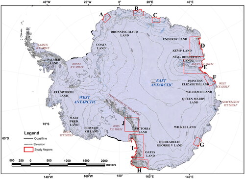
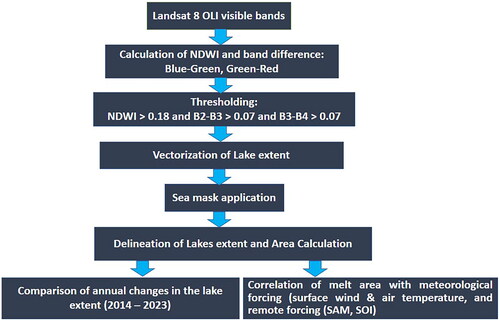
Figure 2. Methodology flowchart adopted in this study (Moussavi et al. 2020).

On the East Antarctic, regions D, E, and F (corresponding to 157,151, 194,318, and 46,502.4 km²) encompassed a sizable portion of the margin. These are dispersed across the Princess Elizabeth Land, Mac. Robertson Land, Kemp Land, Cosgrove Ice Shelf, Amery Ice Shelf, West Ice Shelf, and Shackleton Ice Shelf. The AIS, located in East Antarctic, is the most enormous ice shelf in terms of area, with a staggering surface area of 62,620 km² (Foley et al. 2013). It is the largest glacier drainage basin in the world, draining around 16% of the East Antarctic ice sheet and considerably impacts ocean circulation (Fricker et al. 2002). The AIS's surface melting, which creates a sizable supraglacial drainage system, is notable. According to Spergel et al. (2021), this system consists of multiple interlinked lakes connected by surface waterways. Though larger than region C, the research region G, which has an area of 30042 km² has received less attention in previous melt investigations. The region includes a portion of the Bell Ice Shelf and the Moscow University Ice Shelf. Due to their undulating terrain, the regions H (area: 85,505.8 km²), I (area: 161,734 km²), and J (area: 140,251 km²), which make up a substantial portion of the Transantarctic Mountains, present a difficulty for melt research. It also covers some parts of the eastern margins of the Ross Ice Shelf. The melt over this part is influenced by strong Föhn winds (Ghiz et al. 2021).

Data and pre-processing

This work uses indices and other image-based computations to identify SGLs in the Antarctic using optical image-based lake detection during 2014–2023 (Figure 2). Many datasets are available for these analyses, but not all are appropriate for all investigations due to the restrictions (Table 1).

The images are taken for the summer months of January and February and very few for December were used in this study. The images with a cloud cover of less than 20% were used. The data was further pre-processed and used for the analysis. The study utilized visible bands of Landsat-8 Operational Land Imager at 30 m spatial resolution (Blue band, B2: 0.450–0.515 µm, Green band, B3: 0.525–0.600 µm, and Red band, B4: 0.630–0.680 µm) (Yang and Smith 2013; Pope et al. 2016; Moussavi et al. 2020). Surface meteorological data includes 2-m air temperature, 10-m northward and eastward wind components (monthly, area averaged) plotted using Modern-Era Retrospective analysis for Research and Applications, version-2 (MERRA-2) with a spatial resolution of 0.5° x 0.625°. It provides data from 1980 to date. Elevation was taken from the Reference Elevation Model of Antarctica (REMA), with a spatial resolution of 200 m (Howat et al. 2019). The sea mask shape file provided by Scientific Committee on Antarctic Research (SCAR) was used (https://data.bas.ac.uk/collections/e74543c0-4c4e-4b41-aa33-5bb2f67df389/).

Threshold-based lake classification

We computed the Normalized Difference Water Index (NDWI) using blue and red bands. NDWI performs well in identifying SGL in Antarctica, using either near infrared and green bands, or blue and red bands (Xu 2006; Morriss et al. 2013; Moussavi et al. 2016; Williamson et al. 2017; Stokes et al. 2019). Open water features appear as a dark blue colour in optical satellite images due to the rapid attenuation of red light in water relative to blue light. NDWI ratios are, therefore, well suited to map lakes, as they exploit the properties of lakes which make them more easily distinguished from ice at short optical wavelengths (blue wavelengths), and from snow at long optical wavelengths (red wavelengths) (Box and Ski 2007; Sneed and Hamilton 2007; Liang et al. 2012; Morriss et al. 2013; Yang and Smith 2013; Pope et al. 2016; Moussavi et al. 2020). The threshold of above 0.18 is taken into consideration for the detection of MW lakes in order to reduce misclassification of slush and blue-ice pixels (Moussavi et al. 2020). $$\mathrm{\text{NDWI}}=\frac{\mathrm{\text{Blue}}–\text{Red}}{\mathrm{\text{Blue}}+\mathrm{\text{Red}}}$$

The difference between blue and green (B2-B3) bands and green and red (B3-B4) bands was also calculated. These differences removed shaded snow and cloud shadows from the final output. Thresholds above 0.07 are utilized (Moussavi et al. 2020). The areas where all these values are available are taken. This prominent method of SGL detection over the Antarctic using Landsat-8 visible bands is more adopted by Moussavi et al. (2020). The NDWI mentioned above, other than the traditional one, is used here because of the sensitivity of the blue band.

Manual delineation of lakes and post-processing

In the post-processing, the output is further masked with the sea mask layer obtained from the SCAR (BAS Data Catalogue, https://catalogue-testing.data.bas.ac.uk/master/). The results are vectorized and the lakes having areas smaller than 10000 m² are removed. This is done to keep the focus on comparatively larger lakes and melt and remove some of the associated errors during the lake detection and further in the vectorization of the final output image. Eventually, the lakes are delineated manually, and their area and extent are calculated in all the different years within the decade. These lakes are compared with the SCAR database and with those identified by Stokes et al. (2019) to get an inventory of previously identified lakes (before 2007) and also to account for the recently formed lakes.

We computed Pearson correlation coefficient to test the hypothesis of whether two variables are correlated, with an assumption that the joint distribution of the variables is normal. It has been shown that the correlation coefficient is quite robust with regard to this assumption, meaning that Pearson’s correlation coefficient may still be validly estimated in skewed distributions (Havlicek and Peterson 1977). The correlation between two variables yields a p-value indicating the chance of finding the correlation coefficient’s observed value or any value indicating a higher degree of correlation, given a null hypothesis that the two variables are not actually correlated. Though the correlation coefficient does not vary depending on sample size, the p-value yielded with the t-test do. As is a common practice, we use p < 0.05 to test our computations.

Errors and uncertainties in melt lake extraction

Major uncertainties can be caused by atmospheric factors such as cloud cover, topographic features such as rock shadows, and the season for which the data is collected (Moussavi et al. 2020). To mitigate these errors, researchers can cross-check the data with ground truth data or high-resolution imagery for the area. Another effective but time-consuming method is the manual digitization of melt lake boundaries (Stokes et al. 2019; Moussavi et al. 2020). This method of digitizing each single lake is employed in our research alongside automated methods, such as cloud, rock and seawater masks, to reduce errors (Moussavi et al. 2020). Additionally, lakes covering less than 0.01 km² are removed to avoid errors caused by shadows of elevated features, such as rocks, which often blend with the reflectance of melted lakes. Precisely quantifying these errors is challenging due to the lack of ground truth data and high-resolution imagery for the entire area. However, the employed techniques have significantly reduced these uncertainties in our study.

Results and discussion

Melting and freezing of the SGLs over the years

Surface water bodies typically melt over the Antarctic before refreezing. According to Arthur et al. (2020) and Stokes et al. (2019), the austral summer is usually when the melt occurs at the margins and environs. However, these conditions are not continuous throughout the entire season. Furthermore, melting conditions for the same period in a different year may alter. As a result, the amount of melt may change (increase or decrease) from year to year. Such melt studies help assess the effects of global warming. These instances are presented below with the aid of melt found in various Antarctic regions throughout various years. Analysis reveals that there has been a decrease in the melt during the last two to three years. The scenario is also seen in other research areas. Due to the complicated behavior of the several contributing components, including temperature, wind, precipitation, and other factors, it is impossible to pinpoint a single causal factor accurately.

From the distribution (Figures 3–12), it is observed that there are significant differences in the extent of the melt lakes over the years. These differences are partially caused by quick transition of SGL from melting to freezing to melting in just a few days. Consequently, it took time to determine the precise lake extent consistently. Another issue was that we had to switch to the best substitute because the images were unavailable for the same period of an area. We also faced similar issues. It was targeted to get images with less than 20% cloud cover for January, which is the best time to detect the melted SGLs. As a result, the outcomes may change depending on the time that was considered. In the Dronning Maud Land (Region A), which covers an area of 30270.1 km², we detected 198 lakes, and the extent of the melted SGLs was 100.44 km² (mean of 0.51 ± 4.34 km²). Prior to 2007, SCAR has not reported any lake in this region. Like the other region, the lakes in this location showed signs of additional enlargement and eventually merged to form a larger lake. This is demonstrated by the fact that the lake area revealed in the current study is nearly twice as large as that discovered by Stokes et al. (2019), which was 52.41 km² in total and had 1220 lakes. The situation in Region B was also the same. A total of 140 lakes were found over the 40156.8 km² study area, which covered an area of 256.11 km².

Figure 3. Map represent the detected melt lakes at region A. Lakes in the same area identified by Stokes et al. 2019 and SCAR are also shown. Images A1, A2, and A3 indicate the extent of melt lakes detected between 2014 and 2023, which were detected during January and February.

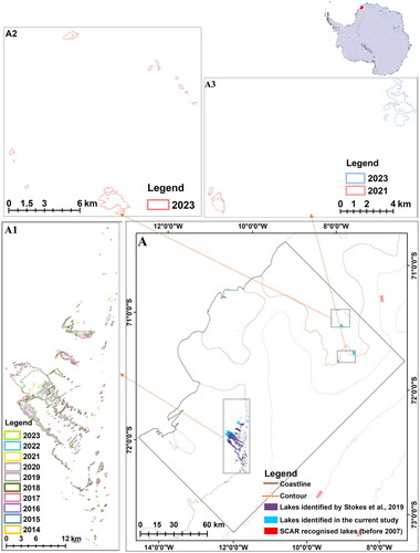
Figure 4. Distribution of lakes in Region B and the melt lakes identified recently (Stokes et al. 2019). Note that the extent of melt lakes increased further for those previously identified and at the new locations over the years. The associated images (B1, B2, and B3) highlight the expansion of the lakes in different years.

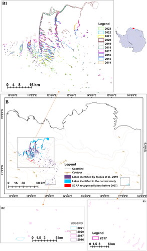
Figure 5. Distribution of melt lakes in Region C. The zoomed images (C1 and C2) showed the temporal extent of the lakes.

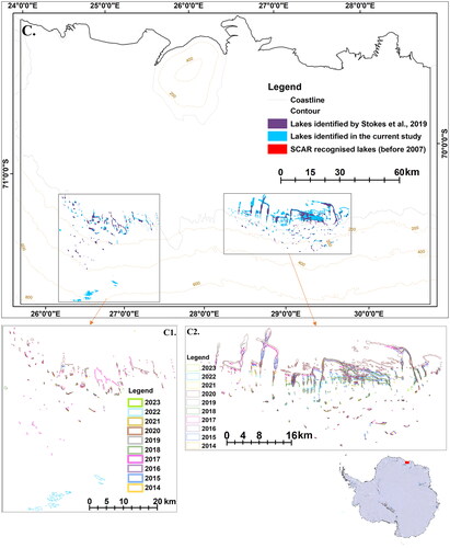
Figure 6. Distribution of melt lakes around Kemp Land margins in Region D. The melt distribution is not towards the interior. Total melt occurred at 11.48 km², which was much less than the other areas in the East Antarctic. No melt was detected for years at many patches (D5 to D8).

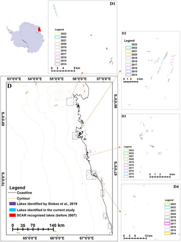
Figure 7. Distribution of melt lakes around the Amery ice shelf, East Antarctic. Note high melt cases in the image (panel E), which shows the melt areas identified by SCAR and Stokes et al. (2019). The melt in the area was detected for most of the years. This region is more prone to melt because of the lesser elevation.

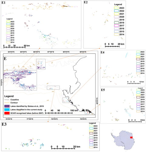
Figure 8. Melt lake distribution at the Mac. Robertson Land, East Antarctic (Region F). Note that this area does not have large melt lakes.

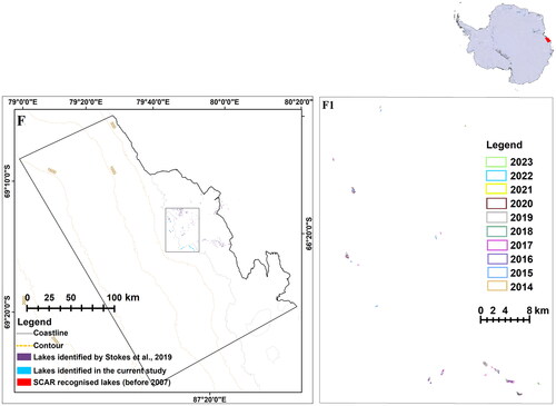
Figure 9. Distribution of melt lakes at the Wilkes Land (Region G). Note that extensive melt was observed during 2014, 2015, and 2020. The melt in the interior was observed at patch (G3) in 2014.

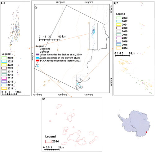
Figure 10. Distribution of melt lakes in the Transantarctic Mountains and environs (Region H). Significant variations in the terrain made detecting lakes difficult in this region.

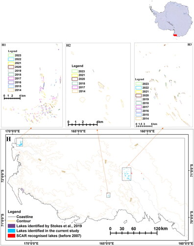
Figure 11. Distribution of melt lakes in the Transantarctic Mountains and at the margins of the Ross Ice Shelf (Region I). The distribution includes melt lakes detected in the past (as documented by SCAR) and in recent years.

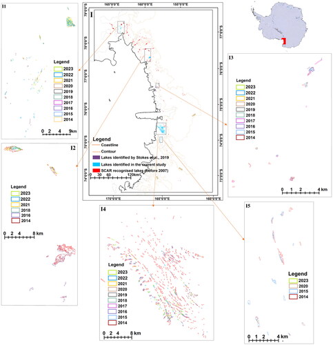
Figure 12. Distribution of melt lakes over the undulated terrain that is a part of the Transantarctic Mountains (Region J). Note that the melt patch (marked as J1) recorded the melt for many years compared to the other patches.

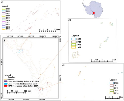
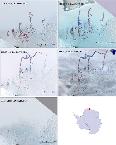
Figure 13. Changes in the melt patterns and their extent at Dronning Maud Land. Note that the melt extent has been expanding north since 2015, and a significant melt occurred in mid-January 2020. The melt is so significant that the horizontal branch of it (at the top) extends to more than 45 km, but in January 2023, the melt is not so remarkable. The average 2-m air temperature for January and February was −8.86 for 2015, −7.27 for 2017, −7.8 for 2018, −7.53 for 2020, and −9.19 for 2023. 

In this work, a total of 639 lakes were detected covering an area of 520.79 km² over Dronning Maud Land. On the other hand, Stokes et al. (2019) identified 5283 lakes covering an area of 190.23 km², while the SCAR database (identified by several scholars before 2007) showed 101 lakes covering an area of 9.15 km². In the East Antarctica, 1025 lakes covering 272.82 km2 were traced, compared to 27982 lakes covering 938.47 km² reported by Stokes et al. and 64 lakes covering 122.07 km² in the SCAR database. In the Transantarctic Mountains and at the eastern margin of the Ross Ice Shelf, Stokes et al. discovered 20 lakes with an area of 5.37 km², and the SCAR database showed 407 lakes spanning an area of 124.18 km², we mapped 1045 lakes with a total area of 93 km². Nevertheless, the total lakes detected in the present investigation account for an area of around three times as large as those detected by Stokes et al. However, this analysis did not include lakes with an extent of less than 0.01 km².

Table 2 provides a summary vis-à-vis the comparison with the SCAR database and Stokes et al. (2019). The scenario is more or less similar for almost all the areas other than those for the Transantarctic Mountains and the surrounding environs. This could be possibly due to less melting over the region over time than otherwise. Dronning Maud Land and East Antarctic regions were more prone to melting due to their less elevated coasts and favorable weather, like warm winds. There is a relationship between 2-m air temperature and melt in these environs (Figure 13). This connects to how the atmospheric elements, specifically for the East Antarctic, affect the melting process. It is clear from several studies published in the past that a variety of factors, including winds (Zou et al. 2019; Dirscherl et al. 2021), air temperature (Picard et al. 2007), precipitation (Dirscherl et al. 2021), surface albedo (a prominent example of which is the Dronning Maud Land), contribute to the surface melt. It may be affected directly or indirectly by the above factors. The situation is much more complicated than it appears to be. Using correlation analysis, several investigators have found that the cause of melt depends on the location (Dirscherl et al. 2021). These elements also reinforce one another.

Table 2. Summary of the total area considered in the study along with the melt area. For comparison, we have listed the melt areas from the recent studies done for the same Regions (Figure 1) in the recent past with the same dataset and almost similar algorithm.

		Current study			Stokes et al. (in 2017)			SCAR (before 2007)
Study area	Total area (km²)	No. of lakes	Area (km²)	Area (%)	No. of lakes	Area (km²)	Area (%)	No. of lakes	Area (km²)	Area (%)
A	30270.1	198	100.44	0.332	1220	52.41	0.173	0	0	0
B	40156.8	140	256.11	0.638	3393	85.73	0.213	101	9.15	0.023
C	27336.1	301	164.24	0.601	670	52.09	0.19	0	0	0
D	157151	109	11.48	0.007	870	9.52	0.006	9	1.42	0.001
E	194318	602	218.7	0.112	26291	916.71	0.472	55	120.65	0.062
F	46502.4	24	2.63	0.006	550	1.4	0.003	0	0	0
G	30042	290	40.01	0.133	271	10.84	0.036	0	0	0
H	85505.8	249	20.28	0.024	0	0	0	20	5.37	0.006
I	161734	689	62.3	0.038	0	0	0	318	100	0.061
J	140251	107	10.32	0.007	20	5.37	0.004	69	18.81	0.013
Total	913267.2	2709	886.51	0.097	33285	1134.07	0.124	572	255.4	0.028

Bold values mention the aggregate results of the study.

The amount of melt can increase if the air temperature rises (Supplementary Figure 4). For example, if the winds are swift, they can expose surface hollows. Likewise, when the cold katabatic winds sweep the surface, they warm up adiabatically and increase the surface melt (Doran et al. 1996). Similar circumstances apply to Föhn winds, which raise the temperature when they descend along a slope on the leeward side of mountains. These winds aid snow removal from depressions and erode the surface, creating moulins (vertical ice shafts) and crevasses that get filled with the MW that moves toward the ice sheet’s base. The MW on the ice surface decreases the albedo (reflectivity) and absorbs solar radiation (Perovich and Tucker 1997; Lüthje et al. 2006), which aids in the further melting and enlargement of the lakes. Although this instance is more typical with the debris-covered glaciers, the rise in turbidity in the lake water can also cause a decrease in albedo (Mertes et al. 2017).

Notably, the Dronning Maud Land region experiences a higher proportion of melt than other regions investigated in this work. Specifically, Regions A, B, and C constitute 0.332%, 0.638%, and 0.601% of the total study area, respectively, making them the most vulnerable regions to melt among the regions investigated. The melt percentage for Regions A, B, and C were 0.173%, 0.213%, and 0.19%, respectively, for 2017 (Stokes et al. 2019). These values are roughly half or one-third of the values obtained in the present study, indicating a significant increase in melt activity. The SCAR database shows no melt activity for Regions A and C, except for Region B, where a minimal melt activity is reported (0.023%). The strong positive correlation of melt area with 2-m air temperature for Region B and C was found to be 0.781 (p < 0.01) and 0.817 (p < 0.01), respectively, while for Region A, it was 0.32. For the years considered in this work, a correlation coefficient greater than 0.632 is significant (p < 0.05). This suggests that the air temperature played a crucial role in the melt in the Dronning Maud Land.

Several factors, including SAM, could influence the rise in air temperature. The latter strongly relates negatively to melt (Tuckett et al. 2019). The more negative the SAM value, the more pronounced the melt (Supplementary Figure 5). The correlation coefficient between SAM and melt area for Regions A, B, and C was found to be −0.1048, −0.64, and −0.679, respectively (Table 4). Based on this relation, the negative phase of SAM significantly impacts the Dronning Maud Land surface melt. As for other Regions, all except Region E exhibited a greater extent of melt in the current study compared to that identified elsewhere (Stokes et al. 2019). Region E primarily covers the AIS, and the images used for melt detection were recorded for January and February, not confined to a single week or month. Predicting the exact amount of melt for any year is highly uncertain, as it can vary over periods and may be less precise when images cover larger periods.

For Region D, there was no significant variations in the melt area inferred in the present study and that in Stokes et al. (2019), but it differed substantially from SCAR's record. The present study detected 0.007% (11.48 km²) of the total area, while it was 0.006% in Stokes et al. study and just 0.001% according to the SCAR database. With a strong positive correlation of 0.606 between melt and air temperature, it is evident that temperature was a significant driver of the melting process.

The melt area was relatively small for Region F in any of the studies. It was just 0.006% (or 2.63 km²) in the current study and 0.003% for Stokes et al. with no melt reported in the SCAR database. Region G (East Antarctic margins), is a relatively small region, so the proportion of melt was 0.133% in the current study and 0.036% in Stokes et al. Unlike the other regions, Regions H to J was characterized by undulated terrain, and the contributing factors for melt vary. Region H covered a smaller part of this undulation than Regions I and J. The melt lakes area was 0.024%, 0.038%, and 0.0007% for Regions H, I, and J, respectively, however no melt lakes were identified by Stokes et al. in Region H and I, expect for Region J where only 0.004% melt was detected. A positive correlation of 0.70 between melt area and air temperature was found for Region H, which was negative for Regions I and J. This discrepancy can be attributed to the rapidly changing elevation, which affects the manifestation of values. Though the correlation was more than 0.4 (p < 0.01) for Region E-G, it is insignificant for other regions, except for H (R = 0.7). We found a negative correlation for Regions I and J (R<−0.4). A high correlation was detected between 10-m eastward wind and the melt area for Regions I and J, with R values of 0.434 and 0.481, respectively, which are the highest among all the regions.

Northward wind component in the elevated region (Region I and J) have a high correlation (R > 0.3) were found. Likewise, the correlation with the 10-m east wind component (R > 0.43) for Regions I and J is due to Föhn winds and katabatic winds that warm up adiabatically along the leeward side of the elevated features and initiate melt. SOI is found to be negatively correlated with ice melt in Regions B, C, E, and F (R< −0.367) but positively correlated with Region J (R = 0.6) (p < 0.01) and I (R = 0.21, not significant).

Melt area discrepancies and role of local forcing on melt

In total, 913267.2 km² of area was covered in this work. Of the total lake area of 886.51 km², we identified 2709 lakes having an area of more than 0.01 km². In contrast, the total area of the 33285 lakes Stokes et al. (2019) found is 1134.07 km². This is clear from the fact that they worked on a larger area and that the lake’s minimum size was likewise lower. The reason for taking more lakes into account is that their findings include a lot of smaller lakes. They found 65459 lakes in the Antarctic, predominantly in the East Antarctic, of which 58325 have an area of less than 0.01 km². The area calculated in this work is greater than the other two records for most areas (Table 2). The observational period is crucial because the duration for which the SGLs remain is melt condition is varies by a few days. Even though the austral summers last from November to February, the melt occurs most frequently in the middle of January. The inability to obtain cloud-free images during the melt episodes is a crucial factor in the discrepancies in the calculated area. Another source of error is inclusion of lakes with smaller areas SCAR's lakes database has a reasonably small number of lakes. This might be related to how long the lakes were found to exist. All of those records pertain to the time frame before 2007.

We explored the relationship between lake-melt area and 2-m air temperature, 10-m eastward and northward wind components, and compared with the other studies (Figure 13). For the 2-m air temperature monthly area-averaged values, the average of January and February is considered for all the demarcated regions. The melt lake area and the 2-m air temperature are positively correlated for most regions, except for Regions I and J (Supplementary Figure 4). The negative correlation values for Region I and J could be attributed to the Transantarctic Mountains, which impede the effective manifestation of 2-m air temperature. The satellite’s capacity to gather data was soon hindered by the elevation and surface undulations. Earlier studies conducted in the region have found that the melting was caused by a spike in temperature and several coexisting conditions, including strong winds. Nearly all regions in the Dronning Maud Land and East Antarctica exhibit a strong positive correlation between 2-m air temperatures and melt area (R = 0.817). A positive correlation was found for most of the regions, with R exceeding 0.40 for Regions B to H. On the other hand, we obtained a negative correlation for Regions I and J.

On the other hand, Regions I and J has a strong relationship between winds (see Table 3). The relationship between melt area and wind speed is strongly positive. The descending warm Föhn wind and the cool katabatic winds along the leeward side of the Alps may further contribute to this problem by warming the near-surface air and partially depleting the snow, respectively.

Table 3. Correlation values of the melt area with 2-m air temperature, 10-m northward and eastward wind for all the polygons shown on Figure 1. The correlation is strongly positive for all Regions other than Regions I and J which are located around the Transantarctic Mountains. Wind components do not have any correlation with the melt area, except for Regions I and J.

Pearson correlation coefficient
Study area	2m air temp.	10m northward wind	10m eastward wind
A	0.32	−0.106	0.066
B	0.781	−0.357	0.196
C	0.817	0.3	0.316
D	0.606	0.259	−0.396
E	0.455	−0.045	0.049
F	0.516	0.31	0.214
G	0.426	0.115	−0.597
H	0.701	−0.079	0.299
I	−0.385	0.376	0.434
J	−0.437	0.447	0.481

Role of remote forcing on melt

The zonal pressure difference between latitudes 40°S and 65°S serves as the foundation for the Southern Annular Mode (SAM). The positive values of the index correspond to westerlies that are weaker than usual in the mid-latitudes (30°S-50°S) and stronger than average across the mid-high latitudes (50°S-70°S). The SAM index is a commonly used statistic that is made monthly. Simply by averaging the results, it can be utilized seasonally and annually. SAM variability significantly affects Antarctic surface temperatures, ocean currents, and other Southern Hemisphere climate factors. The SAM's phase changeability significantly influences the temperatures along East Antarctica’s coast (Turner et al. 2020). Annual mean temperatures have been higher when the SAM has a negative value since roughly the middle of the 1970s (Marshall and Thompson 2016). According to Kwok and Comiso (2002), positive values signify cold anomalies. Additionally, it is the primary mode of variation for the extra-tropical atmospheric circulation and typically accounts for 35% of the total variability in the Southern Hemisphere’s climate (Marshall 2007).

Since there is a strong correlation between the SAM and temperature in the East Antarctic and between temperatures and the melt, it makes sense to compare SAM variability with the melted lakes in the Antarctic. Supplementary Figure 5 and Table 4 display the correlation estimated using this methodology, with high values in some domains. Over half of the study areas had a negative correlation of more than 0.4. This hypothetical situation can be used to predict how the SAM index will react as melt approaches. When the negative association is more robust, there is more melt. Our findings are consistent with projections since the melt should be more extensive in 2017, 2019, and 2020. The melt has increased dramatically during the past three years (Supplementary Figure 3).

Table 4. Correlation between SAM and SOI indices and melt area.

Correlation of melt with indices (SAM and SOI)
Area	A	B	C	D	E	F	G	H	I	J
SAM	−0.1048	−0.64	−0.6794	−0.4353	−0.3215	−0.244	−0.4485	−0.6556	−0.2777	−0.0367
SOI	0.03397	−0.2868	−0.1818	0.0302	−0.06455	−0.3667	0.1561	0.1494	0.2099	0.6008

The Southern Oscillation Index (SOI) is an important metric used to assess the strength of the Walker Circulation, a critical atmospheric circulation pattern in the Pacific Ocean. This index is crucial in monitoring and predicting El Niño and La Niña events, which can significantly impact the Australian region. The SOI is calculated by comparing the surface air pressure differences between Tahiti and Darwin locations. When the SOI maintains sustained positive values above approximately 8, it indicates the presence of a La Niña event. On the other hand, consistent negative values below −8 signal the occurrence of an El Niño event. These sustained values provide valuable information about the prevailing climatic conditions associated with these phenomena.

The SOI exhibits its most significant correlation with Southern Hemisphere climate anomalies in the Pacific sector of the Southern Ocean, notably including the Ross Sea (Stammerjohn et al. 2012; Simpkins et al. 2012). In this region, when the SOI is in its positive phase, it tends to coincide with lower sea-level pressure, cooler surface air temperatures, and cooler sea surface temperatures. Conversely, during the negative phase of the SOI, higher sea-level pressure, warmer surface air temperatures, and warmer sea surface temperatures are commonly observed in this area. These patterns indicate a strong link between the SOI and the climatic conditions in the Southern Ocean’s Pacific sector, specifically regarding air pressure and temperature (Kwok et al. 2016).

The relationship between the SOI and the melt lake area determined simultaneously shows conflicting trends (Table 4). Only four of the regions showed tendency of a negative correlation (insignificant), which may be a result of SOI's negligible influence on melting. However, warmer temperatures and vice versa around the Ross Sea are associated with a negative phase in the SOI. Few studies demonstrate the SOI's direct contribution to the melt or rise in Antarctic temperature caused by these phenomena.

Challenges and recommendations for future research

More research focus in the eastern part of the Antarctic compared to the west could be due to several issues that we faced in this research. The first thing is the elevation difference in the eastern and western parts of the Antarctic. The lower elevation in the eastern part of the Antarctic allows the warm currents to enter the margins and towards the interior, resulting in more melt during summers. The scenario is different in the western Antarctic. Its higher elevation prevents it from recognizable melt cases. The primary reason for cursory research in the western part is those as mentioned above. Along with this, the availability of data and variations in the elevation are significant challenges for detecting melt. The higher features like mountains create a barrier for the satellites to detect the EMR and create shadows in many parts. For such parts, algorithms and indices cause confusion between MW bodies and rock shadows in the ice. Also, the melt lakes under such shadows cannot be detected separately. The clouds are the other problem in the same kind of research. Although, technological development in the recent past, such as SAR, can conquer most of the problems arising in the detection, but it also contains several limitations. The SAR data is available for recent years, and the research for past decades needs to put the optical data into use. Also, many satellites must provide better temporal coverage of all the areas due to their revisit time and scene size. This is a significant barrier for temporal studies as the detection of lakes largely depends on the time period. The lakes remain in melted condition for a few times in the season and imagery for those days is a must. The C-band SAR also does not detect the melt over the blue ice. The researchers employ several techniques, algorithms, indices, and approaches to detect melt in the Antarctic. However, there is only one way to detect the lakes for the entire Antarctic without errors using a single dataset. It could be because of the availability of the datasets, the associated errors, or other issues.

Detecting SGLs in Antarctica using remote sensing and Geographic Information System poses several challenges due to the region’s unique characteristics. The problems are even more when discussing the optical remotely sensed data. Optical data is the only option for more extensive temporal studies in some areas. The SAR observations can overcome many of these challenges, but it is very recent. So, for the studies based on visible bands, several climatic components can be the barrier to make their studies.

In most cases, cloud cover is a large problem for optical image-based analyses. Antarctica is often covered by clouds, particularly during the summer months when SGL formation is most prevalent. Cloud cover obstructs the satellite view and makes capturing clear images of the surface challenging, hindering the detection of SGLs. These clouds can create a shadow above the lake features as well. High reflectance of ice and snow in the visible and near-infrared spectrum can make it difficult to differentiate between water and ice/snow-covered surfaces. This problem is even there with C-band SAR. It can confuse with SGL features and blue ice. Because of this, it is a challenging task to identify and delineate the SGL features from the rest of the features.

The SGL features’ small size and irregular shapes are another challenge in such studies. SGL in Antarctica are often small in size and irregularly shaped. They can be as small as a few meters or less in diameter. Detecting such small features from satellite imagery with limited spatial resolution can be difficult, as they may appear as noise or be missed altogether. Because of this challenge, the lake below 0.01 km² are not included in this study. If the study covers more part of undulated terrain and surface roughness is high, like in the case of the West Antarctic, then it would also be a challenge. The rough and undulating surface of glaciers in Antarctica can complicate the detection of SGLs. Shadows and surface irregularities can interfere with remote sensing techniques, affecting the accuracy of lake detection. Along with these climatic and topographic challenges, there are some challenges from the side of the detecting instrument or satellite sensor.

Different remote sensing sensors have varying spatial, spectral, and temporal resolutions and limitations in their ability to penetrate clouds and detect surface water. The choice of sensor and availability of suitable imagery can impact the effectiveness of SGL detection. The resolution of the satellite itself is a challenge for such kinds of studies. Along with spatial resolution, temporal resolution also matters a lot. SGLs can form and drain rapidly, resulting in temporal variability. Detecting lakes at a specific time may capture only some extent of lake dynamics. Multiple satellite acquisitions or frequent monitoring are necessary to track lake changes accurately.

Once the entire research is done, the final part of ground truth and validation are crucial. Validating SGL detection results with ground truth data is challenging in Antarctica due to its remote and harsh environment. Accessing field measurements and ground truth data for lake presence, size, and duration can be limited. The available options for the ground truth are other good-resolution images and aerial photographs. These can be conquered when new technologies develop better-resolution satellites in the future and advanced remote sensing techniques and algorithms further support it.

Conclusions

There is no clear trend in the melt area in any of the Antarctic regions during the period of analysis. Nearly all areas have exhibited a decrease in melt over the past few years, and the number of melt cases dropped after 2020. The situation is different for 2018 and 2019, where melt was comparatively higher. Even in the East Antarctic (around Kemp Land, Mac Robertson Land, and Princess Elizabeth Land) and Dronning Maud Land and environs, the case was clearly in favour. This is because of the low elevation and minimal surface undulation, which creates ideal melting conditions and for warm winds and currents to infiltrate the region. When katabatic winds descend downward and sweep the East Antarctic ice sheet, they warm the air near the surface, eroding the snow and also exposing the blue ice and firn, all of which eventually leads to surface melt (Lenaerts et al. 2017).

A strong positive correlation between melt area and air temperature was detected for many regions. This demonstrates how closely the melt is related to the warming of air over the Antarctica. The correlation was poor for other regions, particularly for the Transantarctic Mountains, which are locations where the influence of temperature is less but other factors, such as precipitation play a dominant role. The area’s varied geography also cause the satellites’ inaccurate data collection, which may be the reason for a negative correlation. Due to the complicated interplay of numerous elements, it is impossible to pinpoint the precise source of all melt activity.

The study offered an opportunity to understand the SGLs melting in the Antarctic for a decade and map its extent. The results could be used as a benchmark for future studies. Several climatic, topographical, and technological challenges arise during such extensive spatiotemporal studies. Addressing these challenges requires combining advanced remote sensing techniques and image processing algorithms and integrating multiple data sources, including satellite imagery, radar, and passive microwave data. Developing specialized algorithms that consider these challenges and incorporating ancillary data can improve the accuracy and reliability of SGL detection in Antarctica using remote sensing and GIS techniques.

Authors’ contributions

Rahul Pandey: resources, data curation, conceptualization, chart organization, methodology and writing-original draft preparation, writing-review and editing; Alvarinho J. Luis: resources, data curation, chart organization and editing-original draft preparation. All authors have read and agreed to the published version of the manuscript.

Data availability statement

All data supporting the findings of this study are included within the article. Data will be made available from authors on reasonable request.

Disclosure statement

No potential conflict of interest was reported by the author(s).

Correction Statement

This article has been corrected with minor changes. These changes do not impact the academic content of the article.

References

- Arthur JF, Stokes C, Jamieson SS, Carr JR, Leeson AA. 2020. Recent understanding of Antarctic supraglacial lakes using satellite remote sensing. Progr Phys Geograph Earth Environ. 44(6):837–869. doi: 10.1177/0309133320916114.
- Banwell AF, MacAyeal DR, Sergienko OV. 2013. Breakup of the Larsen B ice shelf triggered by chain reaction drainage of supraglacial lakes. Geophys Res Lett. 40(22):5872–5876.,. 2013. doi: 10.1002/2013GL057694.
- Barrand NE, Vaughan DG, Steiner N, Tedesco M, Kuipers Munneke P, Van Den Broeke MR, Hosking JS. 2013. Trends in Antarctic Peninsula surface melting conditions from observations and regional climate modeling. J Geophys Res Earth Surf. 118(1):315–330.
- Bell RE, Banwell AF, Trusel LD, Kingslake J. 2018. Antarctic surface hydrology and impacts on ice-sheet mass balance. Nature Clim Change. 8(12):1044–1052.
- Bell RE, Chu W, Kingslake J, Das I, Tedesco M, Tinto KJ, Zappa CJ, Frezzotti M, Boghosian A, Lee WS. 2017. Antarctic ice shelf potentially stabilized by export of meltwater in surface river. Nature. 544(7650):344–348. doi: 10.1038/nature22048.
- Box JE, Ski K. 2007. Remote sounding of Greenland supraglacial melt lakes: implications for subglacial hydraulics. J Glaciol. 53(181):257–265. doi: 10.3189/172756507782202883.
- Corr D, Leeson A, McMillan M, Zhang C, Barnes T. 2021. An inventory of supraglacial lakes and channels across the West Antarctic ice sheet. Earth Sys Sci Data. 14(1):209–228.
- de Roda Husman S, Hu Z, Wouters B, Munneke PK, Veldhuijsen S, Lhermitte S. 2022. Remote sensing of surface melt on Antarctica: opportunities and challenges. IEEE J Sel Top Appl Earth Observ Remote Sens. 16:2462–2480. doi: 10.1109/JSTARS.2022.3216953.
- Dell R, Arnold N, Willis I, Banwell A, Williamson A, Pritchard H, Orr A. 2020. Lateral meltwater transfer across an Antarctic ice shelf. Cryosphere. 14(7):2313–2330. doi: 10.5194/tc-14-2313-2020.
- Dirscherl M, Dietz AJ, Kneisel C, Kuenzer C. 2020. Automated mapping of Antarctic supraglacial lakes using a machine learning approach. Rem Sens. 12(7):1203.
- Dirscherl M, Dietz AJ, Kneisel C, Kuenzer C. 2021. A novel method for automated supraglacial lake mapping in Antarctica using Sentinel-1 SAR imagery and deep learning. Rem Sens. 13(2):197.
- Dirscherl MC, Dietz AJ, Kuenzer C. 2021. Seasonal evolution of Antarctic supraglacial lakes in 2015–2021 and links to environmental controls. Cryosphere. 15(11):5205–5226.
- Doran PT, McKay CP, Meyer MA, Andersen DT, Wharton RA, Hastings JT. 1996. Climatology and implications for perennial lake ice occurrence at Bunger Hills Oasis, East Antarctica. Ant Sci. 8(3):289–296.
- Drews R, Schannwell C, Ehlers TA, Gladstone R, Pattyn F, Matsuoka K. 2020. Atmospheric and oceanographic signatures in the ice shelf channel morphology of Roi Baudouin Ice Shelf, East Antarctica, inferred from radar data. J Geophys Res Earth Surf. 125(7):e2020JF005587.
- Foley KM, Ferrigno JG, Swithinbank Charles Williams RS, Jr., Orndorff AL. 2013. Coastal-change and glaciological map of the Amery Ice Shelf area, Antarctica: 1961–2004: U.S. Geological Survey Geologic Investigations Series Map I–2600–Q, 1 map sheet, 8-p.
- Fricker HA, Allison I, Craven M, Hyland G, Ruddell A, Young N, Coleman R, King M, Krebs K, Popov S. 2002. Redefinition of the Amery ice shelf, East Antarctica, grounding zone. J Geophys Res. 107(B5):ECV–EC1. doi: 10.1029/2001JB000383.
- Fricker HA, Hyland G, Coleman R, Young NW. 2000. Digital elevation models for the Lambert glacier–Amery Ice Shelf system, East Antarctica, from ERS-1 satellite radar altimetry. J Glaciol. 46(155):553–560. doi: 10.3189/172756500781832639.
- Ghiz ML, Scott RC, Vogelmann AM, Lenaerts J, Lazzara M, Lubin D. 2021. Energetics of surface melt in West Antarctica. Cryosphere. 15(7):3459–3494. doi: 10.5194/tc-15-3459-2021.
- Gong F, Zhang K, Liu S. 2023. Retrieving the grounding lines of the Riiser-Larsen Ice Shelf using Sentinel-1 SAR images. Int J Digital Earth. 16(1):2467–2486. doi: 10.1080/17538947.2023.2229785.
- Halberstadt ARW, Gleason CJ, Moussavi MS, Pope A, Trusel LD, DeConto RM. 2020. Antarctic supraglacial lake identification using Landsat-8 image classification. Remote Sensing. 12(8):1327.,. doi: 10.3390/rs12081327.
- Havlicek LL, Peterson NL. 1977. Effect of the violation of assumptions upon significance levels of the Pearson r. Psychol Bull. 84:373–377.
- Hillenbrand C-D,Bentley MJ,Stolldorf TD,Hein AS,Kuhn G,Graham AG,Fogwill CJ,Kristoffersen Y,Smith JA,Anderson JB, et al. 2014. Reconstruction of changes in the Weddell Sea sector of the Antarctic Ice Sheet since the Last Glacial Maximum. Quat. Sci. Rev. 100:111–136. doi: 10.1016/j.quascirev.2013.07.020.
- Horwath M, Dietrich R, Baessler M, Nixdorf U, Steinhage D, Fritzsche D, Damm V, Reitmayr G. 2006. Nivlisen, an Antarctic ice shelf in Dronning Maud Land: geodetic–glaciological results from a combined analysis of ice thickness, ice surface height and ice-flow observations. J Glaciol. 52(176):17–30. doi: 10.3189/172756506781828953.
- Howat IM, Porter C, Smith BE, Noh M-J, Morin P. 2019. The reference elevation model of Antarctica. Cryosphere. 13(2):665–674.,. doi: 10.5194/tc-13-665-2019.
- Iken A, Bindschadler RA. 1986. Combined measurements of subglacial water pressure and surface velocity of Findelengletscher, Switzerland: conclusions about drainage system and sliding mechanism. J Glaciol. 32(110):101–119.,. doi: 10.3189/S0022143000006936.
- Iken A. 1981. The effect of the subglacial water pressure on the sliding velocity of a glacier in an idealized numerical model. J Glaciol. 27(97):407–421.,. doi: 10.3189/S0022143000011448.
- Kingslake J, Ely JC, Das I, Bell RE. 2017. Widespread movement of meltwater onto and across Antarctic ice shelves. Nature. 544(7650):349–352. doi: 10.1038/nature22049.
- Krawczynski MJ, Behn MD, Das SB, Joughin I. 2009. Constraints on the lake volume required for hydro-fracture through ice sheets. Geophys Res Lett. 36(10):L10501. doi: 10.1029/2008GL036765.
- Kwok R, Comiso JC, Lee T, Holland PR. 2016. Linked trends in the South Pacific Sea ice edge and Southern Oscillation Index. Geophys Res Lett. 43(19):10–295. doi: 10.1002/2016GL070655.
- Kwok R, Comiso JC. 2002. Spatial patterns of variability in Antarctic surface temperature: connections to the Southern Hemisphere Annular Mode and the Southern Oscillation. Geophy Res Lett. 29(14):50–51.
- Lai CY, Kingslake J, Wearing MG, Chen PHC, Gentine P, Li H, Spergel JJ, van Wessem JM. 2020. Vulnerability of Antarctica’s ice shelves to meltwater-driven fracture. Nature. 584(7822):574–578. doi: 10.1038/s41586-020-2627-8.
- Langley ES, Leeson AA, Stokes CR, Jamieson SS. 2016. Seasonal evolution of supraglacial lakes on an East Antarctic outlet glacier. Geophys Res Lett. 43(16):8563–8571. doi: 10.1002/2016GL069511.
- Lea J, Brough S. 2019. Supraglacial lake mapping of the entire Greenland Ice Sheet using Google Earth Engine, [abstract]. AGU Fall Meeting 2019, San Francisco, USA, C31A-1483.
- Leeson AA, Forster E, Rice A, Gourmelen N, Wessem JM. 2020. Evolution of supraglacial lakes on the Larsen B ice shelf in the decades before it collapsed. Geophys Res Lett. 47(4):e2019GL085591. doi: 10.1029/2019GL085591.
- Lenaerts JTM, Lhermitte S, Drews R, Ligtenberg SRM, Berger S, Helm V, Smeets CJPP, Broeke MVD, Van De Berg WJ, Van Meijgaard E, et al. 2017. Meltwater produced by wind–albedo interaction stored in an East Antarctic ice shelf. Nature Clim Change. 7(1):58–62.
- Liang D, Guo H, Zhang L, Cheng Y, Zhu Q, Liu X. 2021. Time-series snowmelt detection over the Antarctic using Sentinel-1 SAR images on Google Earth Engine. Rem Sens Environ. 256:112318.
- Liang Y-L, Colgan W, Lv Q, Steffen K, Abdalati W, Stroeve J, Gallaher D, Bayou N. 2012. A decadal investigation of supraglacial lakes in West Greenland using a fully automatic detection and tracking algorithm. Rem Sens Environ. 123:127–138. doi: 10.1016/j.rse.2012.03.020.
- Lüthje M, Pedersen LT, Reeh N, Greuell W. 2006. Modelling the evolution of supraglacial lakes on the West Greenland ice-sheet margin. J Glaciol. 52(179):608–618. doi: 10.3189/172756506781828386.
- Marshall GJ, Thompson DW. 2016. The signatures of large‐scale patterns of atmospheric variability in Antarctic surface temperatures. J Geophys Res Atmosph. 121(7):3276–3289.
- Marshall GJ. 2007. Half‐century seasonal relationships between the Southern Annular Mode and Antarctic temperatures. Int J Climatol. 27:373–383.
- Mertes JR, Thompson SS, Booth AD, Gulley JD, Benn DI. 2017. A conceptual model of supra‐glacial lake formation on debris‐covered glaciers based on GPR facies analysis. Earth Surf Process. Landform. 42(6):903–914.
- Morriss BF, Hawley RL, Chipman JW, Andrews LC, Catania GA, Hoffman MJ, Lüthi MP, Neumann TA. 2013. A ten year record of supraglacial lake evolution and rapid drainage in West Greenland using an automated processing algorithm for multispectral imagery. Cryosphere. 7(6):1869–1877., doi: 10.5194/tc-7-1869-2013.
- Moussavi M, Pope A, Halberstadt AR, Trusel L, Cioffi L, Abdalati W. 2020. Antarctic supraglacial lake detection using Landsat 8 and Sentinel-2 Imagery: towards continental generation of lake volumes. Rem Sens. 12(1):134. doi: 10.3390/rs12010134.
- Moussavi MS, Abdalati W, Pope A, Scambos T, Tedesco M, Mac Ferrin M, Grigsby S. 2016. Derivation and validation of supraglacial lake volumes on the Greenland Ice Sheet from high-resolution satellite imagery. Rem Sens Environ. 183:294–303. doi: 10.1016/j.rse.2016.05.024.
- Perovich DK, Tucker WB. 1997. Arctic sea-ice conditions and the distribution of solar radiation during summer. Ann Glaciol. 25:445–450.
- Picard G, Fily M, Gallee H., 2007. Surface melting derived from microwave radiometers: a climatic indicator in Antarctica. Ann Glaciol. 46:29–34. doi: 10.3189/172756407782871684.
- Pope A, Scambos TA, Moussavi M, Tedesco M, Willis M, Shean D, Grigsby S. 2016. Estimating supraglacial lake depth in West Greenland using Landsat8 and comparison with other multispectral methods. Cryosphere. 10:15–27. doi: 10.5194/tc-10-152016.
- Pritchard H, Ligtenberg SR, Fricker HA, Vaughan DG, van den Broeke MR, Padman L. 2012. Antarctic ice-sheet loss driven by basal melting of ice shelves. Nature. 484(7395):502–505. doi: 10.1038/nature10968.
- Rignot E, Casassa G, Gogineni P, Krabill W, Rivera A, Thomas R. 2004. Accelerated ice discharge from the Antarctic Peninsula following the collapse of Larsen B ice shelf. Geophys Res Lett. 31(18):L18401., doi: 10.1029/2004GL020697.
- Rignot E, Mouginot J, Scheuchl B, Van Den Broeke M, Van Wessem MJ, Morlighem M. 2019. Four decades of Antarctic Ice Sheet mass balance from 1979–2017. Proc Nat Acad Sci. 116(4):1095–1103.
- Rott H, Müller F, Nagler T, Floricioiu D. 2011. The imbalance of glaciers after disintegration of Larsen-B ice shelf, Antarctic Peninsula. Cryosphere. 5(1):125–134.,. doi: 10.5194/tc-5-125-2011.
- Scambos T, Fricker HA, Liu C-C, Bohlander J, Fastook J, Sargent A, Massom R, Wu A-M. 2009. Ice shelf disintegration by plate bending and hydro-fracture: satellite observations and model results of the 2008 Wilkins ice shelf break-ups. Ear Planet Sci Lett. 280(1–4):51–60. doi: 10.1016/j.epsl.2008.12.027.
- Simpkins GR, Ciasto LM, Thompson DW, England MH. 2012. Seasonal relationships between large-scale climate variability and Antarctic sea ice concentration. J Clim. 25(16):5451–5469. doi: 10.1175/JCLI-D-11-00367.1.
- Sneed WA, Hamilton GS. 2007. Evolution of melt pond volume on the surface of the Greenland Ice Sheet. Geophys. Res. Letts. 34(3). doi: 10.1029/2006gl028697.
- Spergel JJ, Kingslake J, Creyts T, van Wessem M, Fricker HA. 2021. Surface meltwater drainage and ponding on Amery Ice Shelf, East Antarctica, 1973–2019. J Glaciol. 67(266):985–998. doi: 10.1017/jog.2021.46.
- Stammerjohn S, Massom R, Rind D, Martinson D. 2012. Regions of rapid sea ice change: an inter‐hemispheric seasonal comparison. Geophys Res Lett. 39(6) doi: 10.1029/2012GL050874.
- Stokes CR, Sanderson JE, Miles BW, Jamieson SS, Leeson AA. 2019. Widespread distribution of supraglacial lakes around the margin of the East Antarctic Ice Sheet. Sci Rep. 9(1):13823. doi: 10.1038/s41598-019-50343-5.
- Thoma M, Grosfeld K, Lange MA. 2006. Impact of the Eastern Weddell Ice Shelves on water masses in the eastern Weddell Sea. J Geophys Res. 111(C12):C12010. doi: 10.1029/2005JC003212.
- Trusel LD, Frey KE, Das SB, Karnauskas KB, Munneke PK, van Meijgaard E, van den Broeke MR. 2015. Divergent trajectories of Antarctic surface melt under two twenty-first-century climate scenarios. Nature Geosci. 8(12):927–932. doi: 10.1038/ngeo2563.
- Trusel LD, Frey KE, Das SB, Munneke PK, Van Den Broeke MR. 2013. Satellite‐based estimates of Antarctic surface meltwater fluxes. Geophys Res Lett. 40(23):6148–6153. doi: 10.1002/2013GL058138.
- Tuckett PA, Ely JC, Sole AJ, Livingstone SJ, Davison BJ, Melchior van Wessem J, Howard J. 2019. Rapid accelerations of Antarctic Peninsula outlet glaciers driven by surface melt. Nat Commun. 10(1):4311.,. doi: 10.1038/s41467-019-12039-2.
- Turner J, Marshall GJ, Clem K, Colwell S, Phillips T, Lu H. 2020. Antarctic temperature variability and change from station data. Int J Climatol. 40(6):2986–3007.
- Williamson AG, Arnold NS, Banwell AF, Willis IC. 2017. A Fully automated supraglacial lake area and volume tracking ("FAST") algorithm: development and application using MODIS imagery of West Greenland. Rem Sens Environ. 196:113–133, 560. doi: 10.1016/j.rse.2017.04.032.
- Xu H. 2006. Modification of normalised difference water index (NDWI) to enhance open water features in remotely sensed imagery. Int J Rem Sens. 27(14):3025–3033. doi: 10.1080/01431160600589179.
- Yang K, Smith LC. 2013. Supraglacial streams on the Greenland ice sheet delineated from combined spectral-shape information in high-resolution satellite imagery. IEEE Geosci Remote Sens. Letts. 10:801–805. doi: 10.1109/lgrs.2012.2224316.
- Zou X, Bromwich DH, Nicolas JP, Montenegro A, Wang SH. 2019. West Antarctic surface melt event of January 2016 facilitated by Föhn warming. Quar J Royal Meteorol Soc. 145(719):687–704.