Automatic evaluation and optimization of map registration based on feature overlap area ratio

Abstract

Due to the differences in methods for collecting and processing data and map expression forms, two maps from different sources may have deviations in some objective evaluation metrics and fail to reflect the registration accuracy correctly, even though there are no geographic deviations. To address this issue, an objective evaluation metric based on the Feature Overlap Area Ratio (FOA) is proposed to reflect the accuracy of map registration in complex scenes. The proposed method uses different feature extraction methods to binarize different types of maps, and the registration accuracy is determined by calculating the ratio between the feature overlap area and the smaller value of the feature area in the map. The experiments prove that: the FOA metric is highly robust, and not affected by map types, map levels, and registration algorithms. Compared with other objective metrics, there is a stronger linear correlation between the FOA metric and the registration errors. The FOA metric is more sensitive to the errors and reflects the degree of map registration more accurately. Based on the above research, better registration result can be obtained by panning the two registered tile maps until the FOA value is maximized.

Keywords:

• evaluation metric
• tile map
• feature extraction
• registration optimization

1. Introduction

As mediums for preserving geospatial information, maps play important roles in information analysis (Han et al. 2014) and information fusion (Khalil et al. 2018). Maps undergo various kinds of spatial manipulation and analysis, and it is imperative that they have accurate coordinates. Inaccurate coordinate systems in maps require to be registered for subsequent work. Current research focuses on improving the methods of map registration to obtain better registration accuracy (Ma et al. 2017; Li et al. 2019; Ye et al. 2019, 2022). However, an excellent quality metric that correctly and sensitively responds to the changes in registration quality is also essential. It not only improves the evaluation efficiency but also indicates further optimization. This study focuses on the registration evaluation metrics to better reflect the registration results.

Registration accuracy evaluation metrics are mainly classified into subjective evaluation metrics and objective evaluation metrics. Subjective evaluation metrics require the manual selection of key points correspondences between two images and evaluation of the registration results by calculating the difference of key points. However, the evaluation results could be affected by the human eye error, the number and position of key points, etc. These methods are not only time-consuming and labor-intensive (Wang et al. 2004) but also unable to further respond sensitively to the registration results due to the limit of the human eye. This can lead to increased registration accuracy but decreased metric values. Nonetheless, they are not affected by the image type and apply to all image registration accuracy evaluations. Common metrics include root mean square error (RMSE) (Dellinger et al. 2015; Wang et al. 2018; Yang et al. 2019), median error (ME) (Li et al. 2019) and mean square error (MSE) (Huang and Yang 2020) etc. Karantzalos et al. combined the Markov Random Fields (MRFs) and efficient linear programming for multimodal satellite data registration, and manually selected the Ground Control Points (GCPs) to calculate the registration accuracy (Karantzalos et al. 2014). Maria et al. proposed an unsupervised convolutional neural network for remote sensing images alignment and evaluated the registration accuracy by calculating the errors of landmarks (Vakalopoulou et al. 2019). Wu et al. used unsupervised deep learning to register large-scale historical maps and evaluated the registration accuracy by comparing the average misalignment between fixed landmarks (Wu et al. 2022). Jonas and Jochen registered historical maps and OpenStreetMap (OSM) based on content-based image retrieval (CBIR), and experimentally demonstrated that RMSE of registered maps was less than 200 m (Luft and Schiewe 2021).

The selection of objective evaluation metrics is dependent on the type of registered images. In the medical field, Dice coefficients and Dices coefficients are commonly used to evaluate the registration results (de Vos et al. 2019; Kong et al. 2022). The registration images are firstly binarized into foreground (1) and background (0) and then registration accuracy is evaluated by calculating the degree of foreground overlap. To mitigate the negative effects of initial image bias and inhomogeneous bias fields, a new modality independent neighborhood descriptor (MIND) has been proposed for multi-modal deformable registration (Heinrich et al. 2012). In the field of high-resolution remote sensing image registration, traditional objective metrics are the normalized cross correlation (NCC), the mutual information (MI), and the structural similarity index (SSIM). NCC has been used widely due to its robustness to linear strength changes (Chan et al. 2010). However, it is unsuitable for multimodal image matching with complex intensity changes (Ye et al. 2019). MI describes the probabilistic and statistical dependency between images from the perspective of information entropy, the main disadvantage of MI is that it is easily affected by lighting (Parmehr et al. 2014) and ignores the spatial information of adjacent pixels (Suri and Reinartz 2010). Then normalized mutual information (NMI) was further proposed to avoid the influence of uncertainty of image values and variation of edge entropy (Studholme et al. 1999). SSIM assesses the image by comparing the pixel intensities of two images normalized by luminance and contrast (Wang et al. 2004). However, it is sensitive to brightness change and cannot objectively reflect the registration accuracy of complex map scenes. To overcome the dense local self-similarity, a large number of similarity measures based on structure, shape and contour features have been proposed. Ye et al. proposed a dense local self-similarity (DLSS) which uses shape properties, then the similarity between images is measured by calculating NCC of the DLSS descriptors (Ye et al. 2017). Channel features of orientated gradients (CFOG) was proposed based on orientated gradients of images, and it use FFT to speed up the image matching. The method has stronger robustness and higher efficiency (Ye et al. 2019). Then, based on CFOG, multi-scale features and contour mask are combined to suppress the influence of noise and unstructured regions on image registration (Ye et al. 2022). However, the main drawback of such feature descriptors is the lack of scale and rotation invariance. Therefore, Zhu et al. proposed a new feature matching method named R₂FD₂, which combines a repeatable feature detector and a rotation-invariant feature descriptor. It effectively enhances the repeatability and rotation invariance of features (Zhu et al. 2023), but it’s sensitive to scale distortions. These objective metrics don’t require manual intervention on images and utilize only image information and features for batch accuracy evaluations. However, different metrics are only applicable to some specific images.

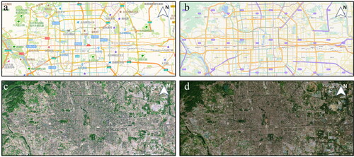
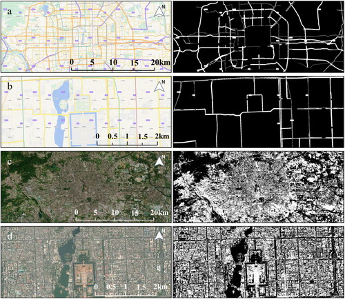
The current state of map registration is characterized by a dearth of objective evaluation metrics. Different source maps exhibit significant differences in visual expression of feature elements in the same area. As shown in Figure 1, there are conspicuous differences in road color, park shape, and color between Figure 1(a) and Figure 1(b), and in vegetation color between Figure 1(c) and Figure 1(d). It isn’t suitable to measure the similarity between maps by intensity and pixel features. However, the structure and shape features are resistant to different map visualization differences. Accordingly, this paper will explore an objective index that is not affected by map color, feature type and text annotation, so as to describe map registration accuracy more accurately.

Figure 1. Representation of different maps of Beijing. (a) Vector map of Amap. (b) Vector map of Tianditu. (c) Remote sensing map of Amap. (d) Remote sensing map of Tianditu.

In this paper, a feature overlap area ratio (FOA) based on shape and structure of the image is proposed for map registration evaluation. We first extract the features of different types of maps by different methods, and binary them to get the feature representation map. Then, the map registration accuracy is determined by calculating the ratio between the overlapping area of the features and the smaller one of them. In addition, based on the existing registration result, the registration accuracy could be optimized by searching for the maximum FOA value in its neighborhood. Accordingly, the main contributions of this paper are as follows:

1. A non-supervised objective evaluation metric for map registration. It can effectively avoid the influence of illumination, noise and text annotation, which combines the similarity of features and structures.

2. The proposed metric can optimize the precision of the registered map.

2. Related work

In this section, we provide a concise overview of the commonly employed objective evaluation metrics for image registration and image binarization methods.

2.1. Objective evaluation metrics

2.1.1. Mutual information (MI)

The development of information theory is based on uncertainty. In this context, scholars have attempted to describe image quality by analyzing the probability of occurrence of pixel values and quantify the image with information. The information entropy was proposed for image evaluation (Studholme et al. 1999). It is commonly assumed that the overlapping region is the largest and the joint entropy is minimized when the two images are fully registered. Based on above theory, mutual information has been used to evaluate image registration accuracy, it is defined as: (1) $$I\left(S_1,S_2\right)=H\left(S_1\right)+H\left(S_2\right)-H\left(S_1,S_2\right)$$(1)

Where $H\left(*\right)$ represent the information entropy of image and $H(S_1,S_2)$ is their joint entropy. $I\left(S_1,S_2\right)$ is the statistical correlation between the two images (Liu et al. 2019) and the larger value represents a stronger correlation and better registration accuracy.

2.1.2. Normalized mutual information (NMI)

To further circumvent the effects of uncertainty in image values and changes in edge entropy on the image registration, normalized mutual information (NMI) was proposed (Studholme et al. 1999) by normalizing the MI to [0, 1]. NMI can reflect the registration accuracy more intuitively. The closer the NMI value is to 1, the better the image registration effect. NMI is defined as: (2) $$\mathit{\text{NMI}}\left(S_1,S_2\right)=\frac{H\left(S_1\right)+H\left(S_2\right)}{H\left(S_1,S_2\right)}$$(2)

2.1.3. Structural similarity index (SSIM)

The Structural Similarity Index (SSIM)was widely used to measure the similarity between two images (Wang et al. 2004), which evaluates the image quality by considering image brightness, structure and contrast. It is defined as: (3) $$\mathit{\text{SSIM}}\left(S_1,S_2\right)=\underset{W_1,W_2}{\mathrm{\text{mean}}}\frac{\left(2{\mu }_1{\mu }_2+C_1\right)\left(2{\sigma }_{12}+C_2\right)}{\left({\mu }_1^2+{\mu }_2^2+C_1\right)\left({\sigma }_1^2+{\sigma }_2^2+C_2\right)}$$(3)

Where $S_1$ and $S_2$ are the reference image and registration image respectively; $W_i$ represents all window patches of the $S_i;$ ${\mu }_i$ is the average value of the windows $W_i;$ ${\sigma }_i^2$ and ${\sigma }_{12}^2$ are the variance of $W_i$ and covariance of the $W_1$ and $W_2$ respectively. $C_1={{(K}_{1}L)}^2$ and $C_2={{(K}_{2}L)}^2$ are the constants to avoid using 0 as the denominator, where $K_1=0.01,$ $K_2=0.03$ and L represents the dynamic range of the image pixel values. SSIM is a value between 0 and 1, the higher value indicates higher similarity between the two images.

2.1.4. Normalized cross correlation (NCC)

For the reference image $S_1$ and the registration image $S_2,$ NCC can be defined as: (4) $$\mathit{\text{NCC}}\left(S_1,S_2\right)=\frac{\sum _{x^{\prime },y^{\prime }}\left(S_1\right(x^{\prime },y^{\prime })-\overline{S_1})\mathrm{*}\left(S_2\right({x+x}^{\prime },{y+y}^{\prime })-\overline{S_2})}{\sqrt{{\sum _{x^{\prime },y^{\prime }}\left(S_1\right(x^{\prime },y^{\prime })-\overline{S_1})}^2\mathrm{*}{\sum _{x^{\prime },y^{\prime }}\left(S_2\right(x+x^{\prime },{y+y}^{\prime })-\overline{S_2})}^2}}$$(4)

Where $S_{\mathrm{*}}\left(x,y\right)$ are the gray value of image $S_{\mathrm{*}}$ at position $\left(x,y\right),$ $x$ and $y$ represent the displacement coordinates of image $S_1$ sliding over image $S_2.$ $\overline{S_1}$ represents the average gray value of the image $S_1,$ and $\overline{S_2}$ represents the average gray value of the overlap area of the image $S_2.$ NCC is a value between −1 and 1, if the value is −1, it means that the two matching windows are completely uncorrelated. On the contrary, if the value is 1, it means that the two matching windows are highly correlated.

The above objective evaluation metrics are not only used for assessing accuracy but also serve as region-based image registration (Jiang et al. 2021). Unimodal images are registered by measuring the distance of the corresponding pixels directly, such as the sum of squared differences (SSD) and the sum of absolute differences (SAD). While, multimodal image registrations rely on statistical comparison of image domains, such as MI and NMI. However, the region registration method based on mutual information has difficulty determining the global maximum of the search space, which reduces the robustness of image registration (Sotiras et al. 2013). Wang et al. (Wang et al. 2020) have demonstrated that SSIM is not suitable for multimodal image registration evaluation due to its lack of detail information.

2.2. Image binarization method

Image binarization is the process of segmenting the image into ‘0’ for the background and ‘1’ for the target (Suh et al. 2022). In remote sensing maps, the common binarization algorithms are the threshold segmentation methods (Thepade et al. 2014), which are classified into global thresholding algorithms and local thresholding algorithms.

The global threshold algorithms divided the image into target and background by calculating the threshold based on the distribution of the overall pixels of the image, common ones are the Otsu algorithm (Otsu 1979) and the maximum entropy method (Li et al. 2022). These algorithms determine the optimal threshold by maximizing interclass variance; however, the amount of calculation is large due to exhaustive searches (Houssein et al. 2021). They are suitable for images with a single gray pixel and a clear bimodal distribution (Wang et al. 2020). The local thresholding algorithms are to first localize the image and then select the appropriate threshold value to distinguish the target and background, such as Niblack’s algorithm (Ding et al. 2023). These methods rely heavily on the selection and processing of the localized window (Xiong et al. 2021). However, they are better than global thresholding to deal with images with uneven illumination, and not effective to deal with images with large differences in the neighborhoods of target pixel points (Guodong et al. 2020). Therefore, a single thresholding algorithm cannot solve the problem of uneven illumination in binarized images. Sun et al. (Guodong et al. 2020) proposed a convolutional neural network approach for solving the problem of complex illumination. The image was preprocessed with the non-local mean filter (NLM) algorithm and binarized based on the improved Bradley algorithm with adaptive weights (Wang, Zhao, et al. 2020). In order to reduce the impact of noise and artifacts, Rusyn et al. used multi-threshold values to binarize remote sensing maps and extract image features (Rusyn et al. 2023).

For color map binarization, the roads of vector maps are binarized based on the color characteristics. Leyk and Boesch made full use of image plane, histogram and color space to extract roads by identifying the pixels of different color layers through a clustering iterative process (Leyk and Boesch 2010). The image was converted from RGB to HIS based on the color theory and then segmented with adaptive thresholding (Zhang et al. 2014).

In conclusion, the remote sensing map is obtained by spacecraft and reflects the reality of the ground object, so there are uneven illumination, shadow and noise. The vector map abstracts the real objects and is composed of symbols and text in the form of points, lines and surfaces after manual processing, so there are no uneven illumination, shadow and noise. Due to the different expression modes of different types of maps, there are differences in color, richness of objects and notes. Therefore, it is difficult to use one method to binarize them, we should combine the image features of the map respectively to achieve the binarize effect.

3. Method

3.1. Feature overlap area metrics

3.1.1. Limitations of classical objective evaluation metrics

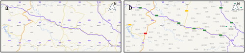
Classical objective evaluation metrics are used to assess the similarity of images by analyzing its internal relationship based on the factors such as the structure, grayscale and pixel information. These metrics apply to images with similar internal structures despite the existence of rotation, translation and local deformation. However, due to the specificity of maps, classical evaluation metrics may produce imprecise results. As shown in Figure 2, where Figure 2(a) is the default representation of Tianditu and Figure 2(b) is obtained by changing the text labeling, feature labeling and road expression of (a). The two maps are equal in size with 1536 pixels * 642 pixels and have no geographic location deviation. Therefore, the RMSE is 0. Ideally the objective evaluation metrics of the two maps should be MI = 1.8782, NMI = 1.0, SSIM = 1.0. However, in actual situations, MI = 1.1919, NMI = 0.6047, SSIM = 0.8461. These evaluation metrics present low similarity and inaccurate accuracy evaluation because the expression forms of the maps are different with the different publishers and there are great differences in the types of features, the number of features, and the color of features presented in the same area.

Figure 2. Maps of the same region with different descriptions. (a) the real map. (b) the test map.

3.1.2. Physical significance of the features

The representation of important geographic information data in maps is a crucial aspect of cartography. However, the same regions are often represented differently in different maps, which can lead to errors in map registrations. To avoid such errors, it is recommended that the representation of important geographic information data should be based on data published by the law and following the guidelines set by relevant authorities. In this paper, such geographically important features are referred to as ‘features’.

In the context of a global similarity criterion, if two range mappings A and B are similar, they are likely to contain overlaps (Pingi et al. 2015). In the field of image registration, the overlapping area is the largest when two images are perfectly registered (Studholme et al. 1999). As shown in Figure 3, the area of its overlapping is also changed when the degree of overlap of two image features (a and b) is changed, the area is maximum until the features are overlapped completely.

Figure 3. Feature change diagram. (a, b) represent features of different images respectively, black area is the overlapping area of features.

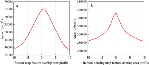
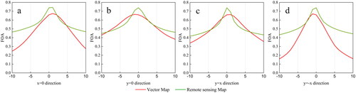
Using the real map in Figure 1 as an example, the features overlapping area of the vector map and remote sensing map are calculated by moving (b) relative (a) and (d) relative (c) respectively, with eastward as positive and westward as negative by 0 to 10 pixels. The distribution curves are shown in Figure 4, it is observed that the overlapping area of the features is maximized when the maps are registered completely.

Figure 4. Variations of feature area overlap.

3.1.3. Calculation formulae of FOA

An unsupervised objective metric based on the feature overlap area ratio (FOA) is proposed under the premise that the feature overlap area is maximized when two maps are perfectly registered. The FOA can avoid the difference of extracted features in maps by calculating the overlap area of them and the fewer area of features is taken as the denominator to guarantee the necessity of it. The FOA is formulated as follows: (5) $$\mathit{\text{FOA}}=\frac{A\cap B}{\mathrm{\text{min}}\hspace{0.17em}\left(A,B\right)}$$(5)

Where A and B represent the area of the feature elements of the reference image and the registered image respectively. The operator ‘$\cap$’ represents the overlapping area of the feature elements of the two images. FOA is a value between 0 and 1, the larger value indicates the better registration result.

In the following, Section 3.2 focus on how to extract the features and calculate the FOA.

3.2. The methods of extracting feature and calculating FOA

3.2.1. Principles for selecting the features

Based the similar principles of subjective evaluation, the selection of geographically significant features is subject to the following conditions:

1. Features must be present in both images;

2. Features must be geographically significant and remain typical and stable;

3. The features must have a certain area and should not be too small.

3.2.2. The process of feature extraction and FOA calculation

The vector maps are composed of point, line and area elements that record geometric and attribute information of the objects (Liu et al. 2022), while remote sensing maps use remote sensing images as base maps to represent geographical phenomena. Therefore, there are the following differences in terms of their form of expression due to the different image characteristics: (1) Vector maps contain a large number of auxiliary elements, such as textual notes and symbolic notes, which are lacking in remote sensing maps. (2) There are temporal and illumination differences in remote sensing maps. Therefore, the features of two types of maps cannot be extracted by the same method. We propose different methods to extract the features of vector maps and remote sensing maps based on their expression forms and characteristics. A specific flow chart is shown in Figure 5.

Figure 5. Flowchart of FOA calculation.

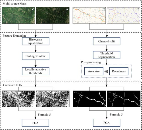
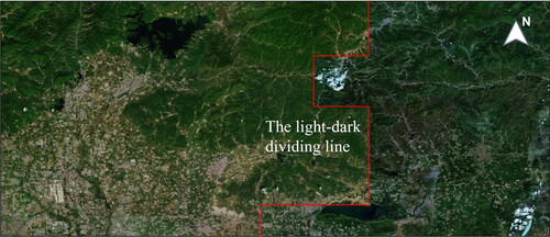
The features of vector maps are extracted by binarization based on its color features, and post-processing operations are carried out on the image to obtain the result maps, such as removing map labels (text and icons) and fine roads. The remote sensing maps are composed of remote sensing images captured at different periods and by different sensors. It may result in variations in map brightness, as shown in Figure 6.

Figure 6. Remote sensing map of Beijing Pinggu district with images from different periods. The left region is light and the right region is dark.

To address the issue of uneven illumination on remote sensing maps, a binarization algorithm for homogenizing illumination is proposed. The proposed algorithm enhances the grayscales of the image to uniform them. Then, it calculates the local adaptive threshold within the range of w*h in the map neighborhood, with pixel point X as the center. The neighborhood range is continuously adjusted until the interclass variance is maximized. The local adaptive threshold at this moment is used as the final threshold of the pixel point X. Finally, binary segmentation is performed. The binarization results of the two types of maps at different scales are shown in Figure 7.

Figure 7. Results of maps binarization at different levels. The left are initial maps and the right are result maps.

3.3. Linear relationship test

3.3.1. Pearson’s correlation coefficient

Pearson’s correlation coefficient (PCC) is used to measure the linear correlation between two variables (Edelmann et al. 2021), which ranges between [−1,1], the larger absolute value implies stronger linear relationship. The PCC of random variable X and Y can be calculated by (6) $${\rho }_{X,Y}=\frac{\mathit{\text{cov}}\left(X,Y\right)}{\sqrt{\mathit{\text{Var}}\left(X\right)\mathit{\text{Var}}\left(Y\right)}}$$(6)

Where $\mathit{\text{cov}}(X,Y)$ is the covariance of $X$ and $Y,$ and $\mathit{\text{Var}}\left(*\right)$ is the variance of the $*.$ For finite N samples {(x₁, y₁) ⋯ (x_n, y_n)}, the PCC can be formulated by (7) $$r_{x,y}=\frac{\sum _{i=1}^N\left(x_i-\overline{x}\right)\left(y_i-\overline{y}\right)}{\sqrt{{\sum }_{i=1}^N{\left(x_i-\overline{x}\right)}^2}\sqrt{{\sum }_{i=1}^N{\left(y_i-\overline{y}\right)}^2}}$$(7)

Where $(x_i,y_i)$ represents the ith sample (0 ≤ i ≤ N), and $\overline{x}=\frac{1}{n}{\sum }_{i=1}^n{x}_i$ represents the sample mean, and similarly for $\overline{y}.$

3.3.2. Confidence intervals

In order to further verify the certainty of the estimated r value in Equation (7)(7) $$r_{x,y}=\frac{\sum _{i=1}^N\left(x_i-\overline{x}\right)\left(y_i-\overline{y}\right)}{\sqrt{{\sum }_{i=1}^N{\left(x_i-\overline{x}\right)}^2}\sqrt{{\sum }_{i=1}^N{\left(y_i-\overline{y}\right)}^2}}$$(7) , we calculate the confidence interval to indicate the possible range of true $\rho$ value on Equation (6)(6) $${\rho }_{X,Y}=\frac{\mathit{\text{cov}}\left(X,Y\right)}{\sqrt{\mathit{\text{Var}}\left(X\right)\mathit{\text{Var}}\left(Y\right)}}$$(6) . First, a z-score is calculated by applying the Fisher transformation F(∙) (8) $$z=F\left(r\right)=\frac{1}{2}\mathrm{\text{ln}}\hspace{0.17em}\left(\frac{1+r}{1-r}\right)=\mathrm{\text{arctanh}}\left(r\right)$$(8)

Second, given a confidence level 1−α of 95% typically, the critical z-score z_α/2 for the two-sided test can be obtained from the corresponding table. Therefore, the confidence interval for F(ρ) is (9) $$F\left(\rho \right)\in \left[F\left(r\right)-z_{\frac{\alpha }{2}}\mathrm{*}\frac{1}{\sqrt{n-3}},F\left(r\right)+z_{\frac{\alpha }{2}}\mathrm{*}\frac{1}{\sqrt{n-3}}\right]$$(9)

Where n represents sample size, therefore the confidence interval of r would be (10) $$F\left(\rho \right)\in \left[F^{-1}\left(F\left(r\right)-z_{\frac{\alpha }{2}}\mathrm{*}\frac{1}{\sqrt{n-3}}\right),F^{-1}\left(F\left(r\right)+z_{\frac{\alpha }{2}}\mathrm{*}\frac{1}{\sqrt{n-3}}\right)\right]$$(10)

Where $F^{-1}\left(z\right)$ represents the inverse of Fisher transformation of z, which can be computed by (11) $$F^{-1}\left(z\right)=\frac{e^{2z}-1}{e^{2z}+1}=\mathrm{\text{tanh}}\hspace{0.17em}\left(z\right)$$(11)

3.4. FOA-based registration optimization

The two maps registered by the PDR algorithm (Zhang and Deng 2023) are used as test maps in Figure 8, and the FOA curves in the four directions of x = 0, y = 0, y = x, and y=-x are plotted in Figure 9. These can be found that: (1) The FOA similarity curves are smooth, and the overall distributions are symmetrical, and the FOA continues to decrease on both sides of the maximum value; (2) The maximum value of the FOA may not be the result of the existing PDR algorithm, and it may be found in the vicinity of the existing registration result. There is still further optimizing space for existing registration result, and the optimal result is within 5 pixels of the existing result.

Figure 8. Test maps of FOA curve. (a) corresponds to (b), (c) corresponds to (d).

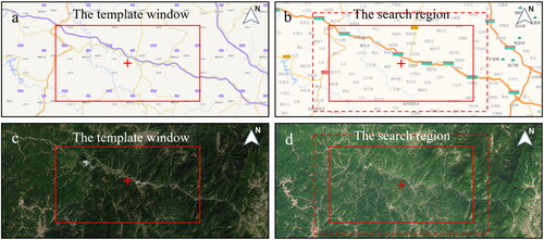
Figure 9. FOA similarity curves.

Based on the feature of FOA similarity curves, the maximum FOA value is searched through the 5-pixel neighborhood range of the existing registered result to optimize map registration result.

4. Experiments

4.1. Data sets

The experimental data are collected from two types of online tile maps include Amap and Tianditu, with Tianditu as the reference map and Amap as the registered map. To assess the impact of different regions on metrics, the study selects Beijing City, Ganzhou City and Shaxi Town, which are representative of the big city maps, small and medium city maps, and town maps respectively. To evaluate the impact of different map scales on metrics, the level 12, level 12.5, and level 13 are selected as the experimental scales. To assess the impact of registration algorithms on metrics, the PDR (Zhang and Deng 2023) and coordinate transformation algorithm are used to register the maps. The coordinates of Beijing City’s center are [116.39, 39.92], Ganzhou City’s center are [114.94, 25.83], and Shaxi Town’s center are [115.58, 26.81]. The map sizes are all 1536 pixels * 642 pixels.

4.2. Experimental setting

We implemented our methods with Python. The experiments were conducted in AMD Ryzen 7 7735H with Radeon Graphics 3.20 GHz and 16.00GB RAM.

4.3. Experimental results

4.3.1. Linear relationship results

Tables 1–3 present the Pearson correlation coefficient (PCC) values between the objective evaluation metrics and registration errors in different areas respectively. The

Table 1. Linear correlation results of metrics and registration error in Beijing city.

	Scale	Algorithm	MI	NMI	SSIM	NCC	CFOG	FOA
Vector maps	12	PDR	0.9359	0.9360	0.9346	0.9749	0.9854	0.9841
		CT	0.9346	0.9348	0.9398	0.9717	0.9938	0.9746
	12.5	PDR	0.9406	0.9406	0.9408	0.9784	0.9966	0.9787
		CT	0.9397	0.9398	0.9403	0.9757	0.9606	0.9725
	13	PDR	0.9638	0.9637	0.9738	0.9858	0.9965	0.9923
		CT	0.9620	0.9621	0.9665	0.9852	0.9966	0.9915
Remote sensing maps	12	PDR	0.8741	0.8541	0.7148	0.9252	0.9948	0.9092
		CT	0.9139	0.9027	0.5804	0.9342	0.9571	0.9271
	12.5	PDR	0.8245	0.8025	0.6949	0.9048	0.9998	0.8811
		CT	0.8808	0.8700	0.5576	0.9132	0.9617	0.9077
	13	PDR	0.8211	0.8055	0.6891	0.8867	0.9966	0.8773
		CT	0.8415	0.8335	0.3775	0.8547	0.9160	0.8591

Table 2. Linear correlation results of metrics and registration error in Ganzhou city.

	Scale	Algorithm	MI	NMI	SSIM	NCC	CFOG	FOA
Vector maps	12	PDR	0.9620	0.9618	0.9520	0.9868	0.9860	0.9823
		CT	0.9644	0.9643	0.9341	0.9943	1.0000	0.9885
	12.5	PDR	0.9632	0.9634	0.9475	0.9828	0.9860	0.9673
		CT	0.9682	0.9684	0.9447	0.9916	0.9966	0.9753
	13	PDR	0.9805	0.9805	0.9444	0.9965	0.9938	0.9871
		CT	0.9805	0.9805	0.9444	0.9965	0.9938	0.9871
Remote sensing maps	12	PDR	0.9132	0.9043	0.7620	0.9486	0.9932	0.9431
		CT	0.9132	0.9043	0.7620	0.9786	0.9932	0.9431
	12.5	PDR	0.9368	0.9279	0.7913	0.9579	0.9938	0.9587
		CT	0.9369	0.9282	0.7776	0.9566	0.9860	0.9588
	13	PDR	0.9324	0.9221	0.8007	0.9575	1.0000	0.9557
		CT	0.9459	0.9377	0.7886	0.9607	0.9938	0.9592

Table 3. Linear correlation results of metrics and registration error in Shaxi town.

	Scale	Algorithm	MI	NMI	SSIM	NCC	CFOG	FOA
Vector maps	12	PDR	0.9638	0.9634	0.9484	0.9910	0.9981	0.9896
		CT	0.9631	0.9626	0.9319	0.9946	0.9966	0.9925
	12.5	PDR	0.9566	0.9556	0.9528	0.9791	0.9933	0.9769
		CT	0.9603	0.9598	0.9479	0.9883	0.9966	0.9821
	13	PDR	0.9652	0.9645	0.9507	0.9740	0.9839	0.9317
		CT	0.9763	0.9761	0.9383	0.9960	1.0000	0.9952
Remote sensing maps	12	PDR	0.8837	0.8751	0.7427	0.9365	0.9966	0.9100
		CT	0.8883	0.8794	0.7435	0.9383	0.9966	0.9126
	12.5	PDR	0.8605	0.8348	0.7347	0.9307	1.0000	0.8915
		CT	0.8972	0.8835	0.7333	0.9455	0.9934	0.9222
	13	PDR	0.8871	0.8761	0.7657	0.9422	1.0000	0.9251
		CT	0.9154	0.9035	0.7236	0.9512	0.9825	0.9381

PCC values in tables represent the average PCC between the errors and the metrics within −10 to 10 pixels in the four directions of x = 0, y = 0, y = x, and y=-x.

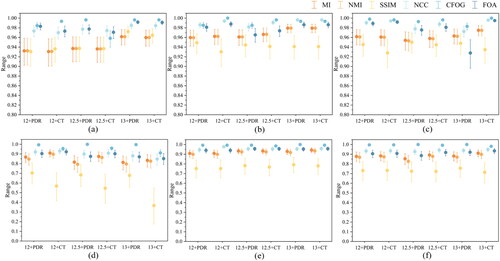
Figure 10 illustrates the distribution of 95% confidence intervals between the metrics and map registration errors. The coordinate transformation algorithm is abbreviated as ‘CT’. The FOA, CFOG and NCC all show high PCC values, and their averages are above 0.95. The mean value of MI and NMI are 0.90 and 0.92 respectively. However, The PCC value of SSIM is the lowest, with a mean value of 0.8294. SSIM shows different correlation affected by the map type, and it shows a higher correlation in the vector maps with a mean value of 0.9463, while a lower correlation in remote sensing maps with a mean value of 0.7078.

Figure 10. Confidence interval charts for different metrics. (a, b, c) represent vector maps of Beijing, Ganzhou and Shaxi, respectively. (d, e, f) represent remote sensing maps of Beijing, Ganzhou and Shaxi, respectively.

4.3.2. Optimization results

4.3.2.1. Impact of registration algorithms

To observe the effect of the registration algorithms to the optimization results, we use two different methods to align maps, and then optimized the map registration accuracy based on the FOA. Remote sensing maps is abbreviated as ‘Rmaps’. Tables 4–6 show the registration optimization values in different areas. The optimized translation values of different maps are kept within 4 pixels, and further improvement of registration accuracy can be achieved by simple translation of the registered maps. For the images registered by different algorithms, the registration results can be optimized to the same accuracy by using the FOA metric.

Table 4. Optimization results of FOA in Beijing City.

Scale	Map	Algorithm	Pre-optimization precision	Panning value(/pixel)	Post-optimization precision	FOA increase value
12	Vector maps	PDR	0.6465	(1, −1)	0.6524	0.0059
		CT	0.5972	(−1, 1)	0.6524	0.0552
	Rmaps	PDR	0.7860	(0, 0)	0.7860	0.0000
		CT	0.6851	(−1, 3)	0.7860	0.1009
12.5	Vector maps	PDR	0.6400	(0, 0)	0.6400	0.0000
		CT	0.5989	(−1, 1)	0.6400	0.0411
	Rmaps	PDR	0.7858	(0, 0)	0.7858	0.0000
		CT	0.6599	(−1, 3)	0.7858	0.1259
13	Vector maps	PDR	0.5753	(0, 0)	0.5753	0.0000
		CT	0.5626	(0, 1)	0.5753	0.0127
	Rmaps	PDR	0.7753	(0, 0)	0.7753	0.0000
		CT	0.6501	(0, 4)	0.7753	0.1252

Note: The panning value (a, b) represents the map has been translated by a pixels in the x-direction and b pixels in the y-direction, as in the table below.

Table 5. Optimization results of FOA in Ganzhou City.

Scale	Map	Algorithm	Pre-optimization precision	Panning value(/pixel)	Post-optimization precision	FOA increase value
12	Vector maps	PDR	0.7021	(0, 0)	0.7021	0.0000
		CT	0.7021	(0, 0)	0.7021	0.0000
	Rmaps	PDR	0.7804	(−1, 0)	0.7815	0.0011
		CT	0.7804	(1, 0)	0.7815	0.0011
12.5	Vector maps	PDR	0.6621	(0, 0)	0.6621	0.0000
		CT	0.6476	(0, −1)	0.6621	0.0145
	Rmaps	PDR	0.7128	(0, 0)	0.7128	0.0000
		CT	0.7036	(0, −1)	0.7128	0.0092
13	Vector maps	PDR	0.6814	(0, 0)	0.6814	0.0000
		CT	0.6739	(1, −1)	0.6814	0.0075
	Rmaps	PDR	0.7434	(0, 0)	0.7434	0.0000
		CT	0.7294	(2, −1)	0.7434	0.0140

Table 6. Optimization results of FOA in shaxi town.

Scale	Map	Algorithm	Pre-optimization precision	Panning value(/pixel)	Post-optimization precision	FOA increase value
12	Vector maps	PDR	0.6736	(0, 0)	0.6736	0.0000
		CT	0.6700	(1, 0)	0.6736	0.0036
	Rmaps	PDR	0.7436	(0, 0)	0.7436	0.0000
		CT	0.7191	(1, 0)	0.7436	0.0245
12.5	Vector maps	PDR	0.6597	(0, 0)	0.6597	0.0000
		CT	0.6586	(0, 0)	0.6586	0.0000
	Rmaps	PDR	0.7630	(0, 0)	0.7630	0.0000
		CT	0.6700	(1, −1)	0.7630	0.0930
13	Vector maps	PDR	0.6867	(0, 0)	0.6867	0.0000
		CT	0.6813	(−1, 0)	0.6867	0.0054
	Rmaps	PDR	0.7486	(0, 0)	0.7486	0.0000
		CT	0.6401	(1, −2)	0.7486	0.1085

4.3.2.2. Impact of optimization metrics

To observe the effect of different metrics to the optimization results, we employ the traditional metrics, including MI, NMI, SSIM, NCC, CFOG to optimize the registration accuracy. In this section, we add more maps of different levels for three regions as experimental data. It is worth noting that the maximum zoom level of remote sensing maps of the Amap and Tianditu can reach 18 levels in urban areas and they can reach 16 level and 18 level, respectively in nonurban areas.

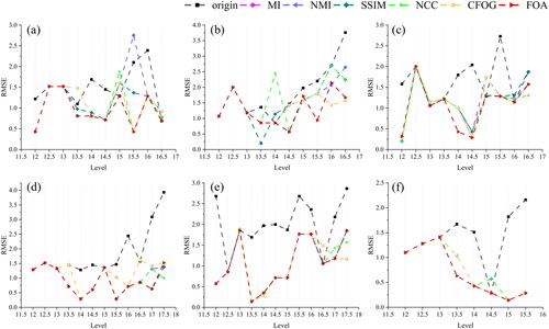
Figure 11 shows the RMSE before optimization and after optimization of the six metrics. Due to the same optimization effect of some metrics, there may be overlapping of broken lines. More original data and panning values at https://github.com/xiaoyan0916/FOA_data.git. In general, one can see that all the metrics can achieve the registration optimization in almost all cases. Compared with other metrics, FOA perform better overall. The perform of SSIM and CFOG are second to FOA due to the RMSE of them are higher than the RMSE of FOA. MI, NMI, and NCC all shows an increase in RMSE after optimization in some cases, which show the worst perform, as shown in Figure 11(a,b).

Figure 11. RMSE after optimization of different metrics. (a) Vector maps of Beijing. (b) Vector maps of Ganzhou. (c) Vector maps of Shaxi. (d) Remote sensing map of Beijing. (e) Remote sensing map of Ganzhou. (f) Remote sensing map of Shaxi.

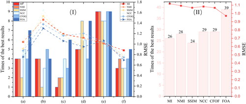
We further count the best performance times of the six metrics in all cases, and calculate their average RMSE, as shown in Figure 12. It can be found that FOA can ensure the map registration optimization to the greatest extent. In terms of the times of optimal performances, FOA performs best in the five scenarios. CFOG is optimized one more time than FOA in Figure 12(I)(b), but the average RMSE of CFOG is higher than FOA. The reason is that CFOG performs poorly at levels 14.5 and 15.5, resulting in a higher average RMSE, combining with Figure 11(b). In terms of average RMSE, FOA also performed best in the five scenarios. This is because FOA achieves the largest RMSE in level 17.5 in Figure 11(e). Overall, FOA achieves the best in both aspects as shown in Figure 12(II). Of the 62 examples, FOA achieves the lowest average RMSE at 0.97. FOA perform the best in 39 examples, accounting for 63% of the total and the optimal performance ratio of the other indicators are all less than 50%.

Figure 12. Average RMSEs and times of the best results for the six metrics in different cases. (I) (a–f) correspond to (a–f) in Figure 11. (II) The sum of times and average RMSE in (I). Bar charts and front charts correspond to times and RMSE.

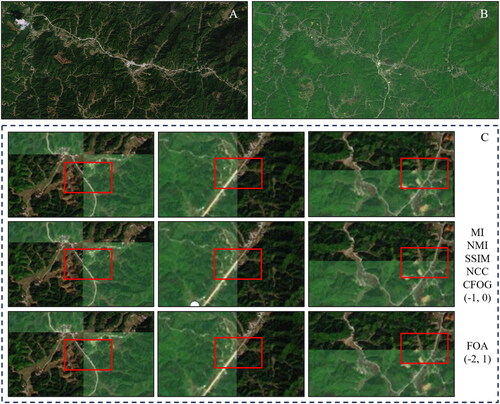
Figures 13–16 show map details after optimization in different regions. After optimization, the connections of important features such as roads and constructions in the maps are smoother, which considerably reduce the misalignment of feature matching and further improve the accuracy of map registration.

Figure 13. Optimization comparison chart of vector map (level 15.5) in Beijing. (A) Tianditu. (B) Amap. (C) The first line represents the maps before optimization, and the 2-4 lines represent the maps after optimization. The optimization metrics and offset values are indicated on the right.

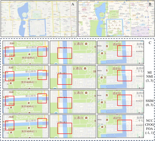
Figure 14. Optimization comparison chart of remote sensing map (level 17) in Beijing. (A) Tianditu. (B) Amap. (C) The first line represents the maps before optimization, and the 2–4 lines represent the maps after optimization. The optimization metrics and offset values are indicated on the right.

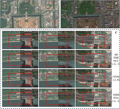
Figure 15. Optimization comparison chart of vector map (level 15) in Ganzhou. (A) Tianditu. (B) Amap. (C) The first line represents the maps before optimization, and the 2–3 lines represent the maps after optimization. The optimization metrics and offset values are indicated on the right.

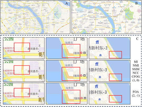
Figure 16. Optimization comparison chart of remote sensing map (level 13.5) in Shaxi. (A) Tianditu. (B) Amap. (C) The first line represents the maps before optimization, and the 2–3 lines represent the maps after optimization. The optimization metrics and offset values are indicated on the right.

4.4. Discussion and analysis

These are known from the above experimental results:

(1) The current objective evaluation metrics can all reflect the error variation, but different metrics have different sensitivity to the error variation. NCC, CFOG and FOA all keep higher correlation with error, the average PCC values are above 0.95. The scope of MI varies depending on maps, and there is the deficiency of uncertain evaluation scope. Although the NMI metric is normalized, it suffers from inaccurate evaluation. This conforms that the information entropy-based methods don’t apply to the registration and evaluation of maps. SSIM is less robust and affected by the type of maps. The correlation between SSIM and the map registration errors is higher in vector maps but lower in remote sensing maps, as shown in Tables 1–3. This is likely because SSIM is determined by the luminance, contrast, and structure of the image, while the uneven distributions of luminance in remote sensing maps lead to a partial bias in the evaluation.

(2) FOA is highly robust and more suitable for the evaluation of map registration. It can improve the accuracy of map alignment, and it’s not affected by map types, map levels and registration algorithms, as shown in Tables 4–6. The larger FOA indicates better registration accuracy, the best registration position can be found when the FOA is maximum by searching on the registered map. Moreover, FOA can optimize maps with different registration degrees to the same accuracy, which reflects the robustness of FOA index.

(3) FOA is more accurate in the evaluation of map registration. Compared with other indicators, FOA can effectively reduce the registration error in different regions, different levels and different types of maps. However, RMSE will increase after optimization for MI, NMI and NCC indicators [Figure 11(a,b,f)]. This confirms that features based on shape and structure are more resistant to map differences than features based on image information entropy and linear relationships. Although SSIM and CFOG can also improve map registration accuracy, the overall optimization effect is worse than FOA. In all scenarios, FOA achieves the lowest average RMSE and the highest number of optimal performances. What’s more, CFOG can have local multi-extremum conditions, which can affect the judgment of the optimal registration results in some cases.

(4) At present, the basic translation operation can satisfy the optimization of map registration in most scenarios. However, the optimization effects are limited by optimization operation methods, due to the inconsistencies in the registration accuracy of different regions in the map. FOA is not restricted by optimization methods.

5. Conclusion

An automatic evaluation method based on Feature Overlap Area Ratio (FOA) is proposed to address the lack of suitable objective evaluation metrics in the map registration. The method avoids the influence of finely changed features on the registration results by calculating the main features extracted by binarization in the map. Compared with classical evaluation metrics such as MI, NMI, SSIM, NCC and CFOG, the linear correlation between FOA and registration errors is stronger. The FOA is highly robust and not affected by map types, map scales and registration algorithms. Furthermore, the registration result is optimized by searching for the maximum FOA value of the registered maps, according to the best registration position can be found based on FOA. The experiments show that FOA can further optimize registration accuracy and it’s more accurate. However, inconsistencies in the registration accuracy of different map regions lead to limited optimization by simple panning operation. It is important to note that FOA can only be evaluated for the registered maps due to completely different feature characteristics in unregistered maps.

The main limitation of the proposed metric is that it cannot address the challenge of map regions with significant deformations. In the future, we will attempt to improve the optimization method.

Acknowledgments

The authors would like to thank the 318 Laboratory of Geoscience and Information Physics.

Disclosure statement

No potential conflict of interest was reported by the author(s).

Data availability statement

These data were derived from the following resources available in the public domain: https://www.amap.com and https://map.tianditu.gov.cn.

Additional information

Funding

This work was supported by National Natural Science Foundation of China under Grant [number 42172330].

References

- Chan JC-W, Canters F, Jianglin M. 2010. Fully automatic subpixel image registration of multiangle CHRIS/Proba data. IEEE Trans Geosci Remote Sens. 48 (7):2829–2839. doi: 10.1109/TGRS.2010.2042813.
- de Vos BD, Berendsen FF, Viergever MA, Sokooti H, Staring M, Išgum I. 2019. A deep learning framework for unsupervised affine and deformable image registration. Med Image Anal. 52:128–143. doi: 10.1016/j.media.2018.11.010.
- Dellinger F, Delon J, Gousseau Y, Michel J, Tupin F. 2015. SAR-SIFT: a SIFT-like algorithm for SAR images. IEEE Trans Geosci Remote Sensing. 53(1):453–466. doi: 10.1109/TGRS.2014.2323552.
- Ding D, Guopeng Z, Jianquan Z, Lanzheng C, Zhou G, Zhang J, Chen L. 2023. Improvement of adaptive Niblack algorithm based on iterative idea. Comput Appl Software. 40(3):308–315. doi: 10.3969/j.issn.1000-386x.2023.03.049.
- Edelmann D, Móri TF, Székely GJ. 2021. On relationships between the Pearson and the distance correlation coefficients. Statist Probab Lett. 169:108960. doi: 10.1016/j.spl.2020.108960.
- Guodong S, Yun X, Liang X, Hang Z, Chenkang L, Yun X, Liang X, Hang Z, Chenkang L. 2020. Binarization method of instrument image with uneven illumination and ghosting. J Appl Optics. 41(1):74–78. doi: 10.5768/JAO202041.0102002.
- Han J-Y, Guo J, Chen YJ. 2014. Registration of vector maps based on multiple geometric features in topological aspects. Survey Rev. 46(336):219–230. doi: 10.1179/1752270613Y.0000000075.
- Heinrich MP, Jenkinson M, Bhushan M, Matin T, Gleeson FV, Brady SM, Schnabel JA. 2012. MIND: modality independent neighbourhood descriptor for multi-modal deformable registration. Med Image Anal. 16(7):1423–1435. doi: 10.1016/j.media.2012.05.008.
- Houssein EH, Helmy BE-d, Oliva D, Elngar AA, Shaban H. 2021. A novel Black Widow Optimization algorithm for multilevel thresholding image segmentation. Expert Syst Appl. 167:114159. doi: 10.1016/j.eswa.2020.114159.
- Huang Q, Yang X. 2020. Subpixel image registration regularised by l1 and l2 norms. IET Image Process. 14(12):2845–2854. doi: 10.1049/iet-ipr.2019.1384.
- Jiang X, Ma J, Xiao G, Shao Z, Guo X. 2021. A review of multimodal image matching: methods and applications. Inform Fus. 73:22–71. doi: 10.1016/j.inffus.2021.02.012.
- Karantzalos K, Sotiras A, Paragios N. 2014. Efficient and automated multimodal satellite data registration through MRFs and linear programming. Computer Vision & Pattern Recognition Workshops. 335–342. doi: 10.1109/CVPRW.2014.57.
- Khalil A, Ng SC, Liew YM, Lai KW. 2018. An overview on image registration techniques for cardiac diagnosis and treatment. Cardiol Res Pract. 2018(15):1437125–1437115. doi: 10.1155/2018/1437125.
- Kong L, Yang T, Xie L, Xu D, He K. 2022. Cascade connection-based channel attention network for bidirectional medical image registration. Vis Comput. 39(11):5527–5545. doi: 10.1007/s00371-022-02678-w.
- Leyk S, Boesch R. 2010. Colors of the past: color image segmentation in historical topographic maps based on homogeneity. Geoinformatica. 14(1):1–21. doi: 10.1007/s10707-008-0074-z.
- Li J, Hu Q, Ai M. 2019. RIFT: multi-modal image matching based on radiation-variation insensitive feature transform. IEEE Trans Image Process. 29:3296–3310. doi: 10.1109/tip.2019.2959244.
- Li L, Han L, Ding M, Liu Z, Cao H. 2022. Remote sensing image registration based on deep learning regression model. IEEE Geosci Remote Sensing Lett. 19:1–5. doi: 10.1109/LGRS.2020.3032439.
- Liu J, Singh G, Al’Aref S, Lee B, Oleru O, Min JK, Dunham S, Sabuncu MR, Mosadegh B. 2019. Image registration in medical robotics and intelligent systems: fundamentals and applications. Adv Intell Syst. 1(6):1900048. doi: 10.1002/aisy.201900048.
- Liu P, Xu X, Yang M. 2022. An improved schema for vector tile map considering symbol integrity. Geomat Inform Sci Wuhan Univ. 47(3):455–462. doi: 10.13203/j.whugis20200033.
- Luft J, Schiewe J. 2021. Automatic content-based georeferencing of historical topographic maps. Transact GIS. 25(6):2888–2906. doi: 10.1111/tgis.12794.
- Ma W, Wen Z, Wu Y, Jiao L, Gong M, Zheng Y, Liu L. 2017. Remote sensing image registration with modified SIFT and enhanced feature matching. IEEE Geosci Remote Sensing Lett. 14(1):3–7. doi: 10.1109/LGRS.2016.2600858.
- Otsu N. 1979. A threshold selection method from gray-level histograms. IEEE Trans Syst Man Cybern. 9(1):62–66. doi: 10.1109/TSMC.1979.4310076.
- Parmehr EG, Fraser CS, Zhang C, Leach J. 2014. Automatic registration of optical imagery with 3D LiDAR data using statistical similarity. ISPRS J Photogram Remote Sens. 88:28–40. doi: 10.1016/j.isprsjprs.2013.11.015.
- Pingi P, Corsini M, Ganovelli F, Scopigno R. 2015. Fast and simple automatic alignment of large sets of range maps. Comput Graph. 47:78–88. doi: 10.1016/j.cag.2014.12.002.
- Rusyn B, Lutsyk O, Kosarevych R, Maksymyuk T, Gazda J. 2023. Features extraction from multi-spectral remote sensing images based on multi-threshold binarization. Sci Rep. 13(1):19655. doi: 10.1038/s41598-023-46785-7.
- Sotiras A, Davatzikos C, Paragios N. 2013. Deformable medical image registration: a survey. IEEE Trans Med Imaging. 32(7):1153–1190. doi: 10.1109/tmi.2013.2265603.
- Studholme C, Hill DLG, Hawkes DJ. 1999. An overlap invariant entropy measure of 3D medical image alignment. Patt Recog. 32(1):71–86. doi: 10.1016/S0031-3203(98)00091-0.
- Suh S, Kim J, Lukowicz P, Lee YO. 2022. Two-stage generative adversarial networks for binarization of color document images. Patt Recog. 130(13):108810. doi: 10.1016/j.patcog.2022.108810.
- Suri S, Reinartz P. 2010. Mutual-information-based registration of TerraSAR-X and Ikonos imagery in urban areas. IEEE Trans Geosci Remote Sensing. 48(2):939–949. doi: 10.1109/TGRS.2009.2034842.
- Thepade S, Das R, Ghosh S. 2014. A novel feature extraction technique using binarization of bit planes for content based image classification. J Eng. 2014:1–13. doi: 10.1155/2014/439218.
- Vakalopoulou M, Christodoulidis S, Sahasrabudhe M, Mougiakakou S, Paragios N. 2019. Image registration of satellite imagery with deep convolutional neural networks. IGARSS 2019 – 2019 IEEE International Geoscience and Remote Sensing Symposium. 4939–4942. doi: 10.1109/IGARSS.2019.8898220.
- Wang K, Zhao L, Huang X, Peng Y, Ma S, Fan H. 2020. A fast binarization method for dark and uneven illumination document images. J Optoelectron Laser. 31(12):1333–1340. doi: 10.16136/j.joel.2020.12.0252.
- Wang L, Shi W, Yang L, Weimin S, Liangliang Y. 2020. Binarization of uneven illumination document image based on gray level fluctuation. Comput Appl Software. 37(12):197–203. doi: 10.3969/j.issn.1000-386x.2020.12.031.
- Wang S, Quan D, Liang X, Ning M, Guo Y, Jiao L. 2018. A deep learning framework for remote sensing image registration. ISPRS J Photogram Remot Sens. 145:148–164. doi: 10.1016/j.isprsjprs.2017.12.012.
- Wang Y, Zhang J, Cavichini M, Bartsch D-UG, Freeman WR, Nguyen TQ, An C. 2020. Study on correlation between subjective and objective metrics for multimodal retinal image registration. IEEE Access. 8:190897–190905. doi: 10.1109/ACCESS.2020.3032348.
- Wang Z, Bovik AC, Sheikh HR, Simoncelli EP. 2004. Image quality assessment: from error visibility to structural similarity. IEEE Trans Image Process. 13(4):600–612. doi: 10.1109/tip.2003.819861.
- Wu S, Schnürer R, Heitzler M, Hurni L. 2022. Unsupervised historical map registration by a deformation neural network. Proceedings of the 5th ACM SIGSPATIAL International Workshop on AI for Geographic Knowledge Discovery. 76–81. doi: 10.1145/3557918.3565871.
- Xiong W, Zhou L, Yue L, Li L, Wang S. 2021. An enhanced binarization framework for degraded historical document images. J Image Video Proc. 2021(13):1–24. doi: 10.1186/s13640-021-00556-4.
- Yang H, Li X, Zhao L, Chen S. 2019. A novel coarse-to-fine scheme for remote sensing image registration based on SIFT and phase correlation. Remote Sens. 11(15):1833. doi: 10.3390/rs11151833.
- Ye Y, Yang C, Zhang J, Fan J, Feng R, Qin Y. 2022. Optical-to-SAR image matching using multiscale masked structure features. IEEE Geosci Remote Sensing Lett. 19:1–5. doi: 10.1109/LGRS.2022.3171265.
- Ye Y, Bruzzone L, Shan J, Bovolo F, Zhu Q. 2019. Fast and robust matching for multimodal remote sensing image registration. IEEE Trans Geosci Remote Sens. 57(11):9059–9070. doi: 10.1109/TGRS.2019.2924684.
- Ye Y, Shen L, Hao M, Wang J, Xu Z. 2017. Robust Optical-to-SAR image matching based on shape properties. IEEE Geosci Remote Sensing Lett. 14(4):564–568. doi: 10.1109/LGRS.2017.2660067.
- Ye Y, Tang T, Zhu B, Yang C, Li B, Hao S. 2022. A multiscale framework with unsupervised learning for remote sensing image registration. IEEE Trans Geosci Remote Sens. 60:1–15. doi: 10.1109/TGRS.2022.3167644.
- Zhang D, Deng J. 2023. Progressive dynamic registration method for tile maps based on optimum multi-features. Applied Sciences. 13(7):4282. doi: 10.3390/app13074282.
- Zhang L, He N, Xu C, Wang J. 2014. Road extraction from color map based on adaptive threshold algorithm in HSI space. J Beijing Union Univ. 28(03):14–19. doi: 10.16255/j.cnki.ldxbz.2014.03.016.
- Zhu B, Yang C, Dai J, Fan J, Qin Y, Ye Y. 2023. R2FD2: fast and robust matching of multimodal remote sensing image via repeatable feature detector and rotation-invariant feature descriptor. IEEE Trans Geosci Remote Sens. 61:1–15. doi: 10.1109/TGRS.2023.3264610.