Interferometric phase diagram generation method based on dot trace texture information and semantic segmentation of correlation coefficients

Abstract

This paper proposes a method for generating interferometric phase diagrams, which includes interferometric image registration based on Dot Trace Texture Information (DTTI) and interferometric phase filtering based on semantic segmentation. First, the InSAR images are sharpened according to the different backscattering characteristics of various pixel values, and DTTI is extracted to generate the Dot Trace Texture Map (DTTM). Second, SIFT feature points are extracted from two InSAR coherent complex images. They are then screened by comparison with DTTI. These selected points are used to calculate the registration relationship, ensuring precise registration of the two images. Third, the interferometric phase diagram is segmented by semantics based on correlation coefficients. For high-quality interferometric phase regions, we use two-dimensional frequency domain rotational symmetric Gaussian Laplace and wavelet domain filters successively. For low-quality regions, we use an average filter to smooth out noise. The superiority of the proposed algorithm was verified through comparative experiments.

Keywords:

• Dot trace texture information
• image registration
• SIFT algorithm
• semantic segmentation
• interferometric phase filtering

1. Introduction

Interferometric synthetic aperture radar (InSAR) measuring technology is widely employed in ground elevation measurement and surface deformation monitoring because of its advantages in extensive coverage, high spatial resolution, numerous available data sources, and all-weather, all-day functionality (Chen et al. 2022). InSAR analyses surface subsidence changes by generating interferometric phase diagram, which contain the interferometric phase information of two InSAR images after registration. The surface deformation can be measured quantitatively by phase unwrapping. In the process of generating interferometric phase diagram of InSAR, two main aspects need to be considered. One is to improve the accuracy of image registration. The other is to reduce the impact of phase noise on the quality of interferometric phase diagram.

Interferometric image registration is an important part of generating interferometric phase diagram. The accuracy of image registration directly affects the quality of the generated interferometric phase diagram, and the quality of the interferometric phase diagram further affects the accuracy of surface settlement detection (Yague-Martinez et al. 2017; Fan et al. 2020; Mao et al. 2021; Men et al. 2022). There are four main types of InSAR image registration methods for currently in use: feature-based registration (Zhang et al. 2019), region-based registration (Reddy and Chatterji 1996), hybrid model-based registration (Yang et al. 2019), and deep learning-based registration (Zhang et al. 2019). Among them, the feature-based registration method is the most popular, which extracts local or global information from prominent features, such as points, lines, and contours. the scale-invariant feature transform (SIFT) (Lowe, 2004) algorithm is a classical feature-based registration algorithm because of its scale invariance, rotation invariance, good accuracy, and robustness, which has been extensively studied and applied. It is still continuously optimized and improved in application.

Many studies have attempted to improve the accuracy of image registration in recent years. Pourfard et al. (2022) proposed a KAZE-SAR algorithm that uses non-linear diffusion filtering to establish the scale level of SIFT descriptors. It can capture the exact location of features in the down-sampling and filtering stages of SIFT, which can improve the localization accuracy and saliency of feature extraction. Zhang et al. (2019) apply a transmission algorithm based on deep learning image analogy to the pre-processing of image registration. The differences in multimodal remote sensing images are eliminated by fusing the master image structure and texture. And the SIFT algorithm is used for final registration. Fan et al. (2020) proposed a fusion framework of a deep residual encoder (DRE) and shallow feature for multi-resolution image registration. It combines the deep and shallow features (SIFT features) for image registration to improve accuracy and overall performance.

In terms of reducing the complexity of image registration, Ordóñez et al. (2021) proposed a hyperspectral maximum stable extremal region (HSI-MSER) algorithm that uses the maximum stable extremal region for image feature point detection and the SIFT algorithm for feature description. It uses less computing resources and gets better image registration results. Ye et al. (2022) proposed a multiscale framework with unsupervised learning for multimodal image registration, named MU-Net. It directly learns the end-to-end mapping from the image pairs to their transformation parameters. Ni et al. (2012) proposed a fully automated registration method based on contours and SIFT. It uses contour features to determine the overlap region and perform coarse and precise registration, improving registration accuracy and reducing runtime.

Image noise has a significant impact on image registration accuracy, therefore effective denoising is necessary. Experts have made many attempts in this regard. Dellinger et al. (2015) proposed a SAR-SIFT algorithm for image registration, and a new gradient definition is introduced to yield an orientation and a magnitude for SIFT feature points that are robust to speckle noise. Xiong et al. (2024) proposed a robust multi-view UAV SAR image registration algorithm based on the selective correlation of the log gradient descriptor for unmanned aerial vehicle (UAV) synthetic aperture radar image registration. This algorithm has developed a log gradient that effectively handles noise in dark areas while resisting speckle noise. Moreover, A histogram of oriented log gradient (HOLG) is designed to weaken the effects of striped radiation noise.

The interferometric phase diagram generated after the registration has varying degrees of noise that needs to be filtered. These noises are generally caused by the influence of thermal noise and decoherence effects on time, space, and frequency. Interferometric phase filtering methods can be generally divided into three categories (Xu et al. 2020): transform domain filtering (also known as time-frequency domain filtering), time domain filtering (also known as spatial domain filtering), and frequency domain filtering. The classical time-domain filtering methods include mean filtering, median filtering, Lee filtering, and improved filtering methods based on them (Xu et al. 2020). Li et al. (2020) proposed an enhanced Lee filtering algorithm based on inverse distance weighting, which provided a better filtering effect in the low coherence, high coherence gradient, and high phase gradient areas of InSAR interferometric phase. The Goldstein filter (Goldstein and Werner 1998) and its improved algorithm (Xu et al. 2020) are representative of frequency domain filtering. Xu et al. (2021) proposed a novel interferometric phase filtering by adopting a local fringe frequency (LFF) compensation technique, and the Goldstein filtering algorithm is used for high-coherence regions, which got the good results in noise reduction and edge preservation. Among the transform domain filtering algorithms, wavelet transform filtering and its improved algorithms are commonly used (Xu et al. 2020). Yan et al. (2021) proposed a fast non-local mean filtering method based on the wavelet packet transform to improve the denoising ability and applicability of the algorithm. Its main includes changing the processing method of the wavelet packet transform, performing wavelet packet coefficient smoothing, and reconstructing the filtered phase using the wavelet packet inverse transform.

The low accuracy of image registration and interference phase noise are the two main reasons that affect the generation of interference phase diagrams. The reason for low image registration accuracy is usually due to the low quality of registered feature points, poor feature point filtering effect, poor selection of geometric transformation models, and interference noise in the image. The quality of interferometric phase diagram is usually affected by signal processing errors, electronic device interference, and radar system noise. We are researching how to generate high-quality interferometric phase diagram. In terms of image registration, research is conducted on how to select feature pairs with high registration accuracy. We analyzed the different scattering characteristics of InSAR electromagnetic waves on different surface coverings, as well as the grayscale probability maps of grayscale images, to preprocess the registration images. Then, extract the dot texture map, which can express the boundary information of high pixel quality objects in the image. We use dot texture information that can contain high contrast and significant texture feature boundary information to guide the screen of SIFT feature points. This method can improve the registration accuracy of InSAR images, reduce computational complexity, and generate the optimal interferometric phase diagram. Due to different surface coverings, the scattering characteristics of InSAR electromagnetic waves are different, and the image quality of different objects is also different. That is to say, there are both high coherence regions and low coherence regions in an image. In terms of interferometric phase region filtering, in order to prevent error diffusion in low-quality interferometric phase regions from causing a decrease in signal-to-noise ratio in high-quality interferometric phase regions, this paper proposes a filtering method that uses the correlation coefficients of two registered images as semantics to divide them into sub regions. By using different filtering methods for different sub regions, the impact of low-quality interference phase regions on high-quality interference phase is weakened, and the overall quality of the interference phase diagram is improved. High quality interferometric phase diagram can be generated through the above two methods.

2. Methodology

In this section, the proposed method is introduced in detail. Our method has four parts: 1) Image pre-processing, which use the image sharpening to remove noises and prominent texture features. 2) Generating DTTM, which extracts image texture details and guide the screening of image feature points. 3) DTTI-SIFT registration, which uses DTTI and an improved SIFT algorithm for image registration 4) Filtering algorithm based on semantic segmentation, which segments the image into different regions according to the image semantics, and uses the different filtering algorithms for the different regions.

2.1. Image pre-processing

It is proved that there is amount of noise interference in InSAR image, which are always generated by different scattering characteristics of InSAR electromagnetic waves according to various ground covers, and influenced by error factors such as the InSAR system itself, baseline inclination, electromagnetic environment, and atmospheric interference (Lu et al. 2007; Zou et al. 2009). This results the low quality of texture information extracted from the InSAR images. Therefore, before generating DTTI, we pre-processed the images with image sharpening to remove noises and prominent texture features.

The principle of image sharpening is to highlight the details and edges of the image by enhancing the contrast between pixels in the image. We adjust the pixel values within a certain grayscale range in the image, scale them to the range of [0,1] through linear transformation, to increase the contrast between pixels within this range and other pixels. This operation enhances the texture details of the image and removes high noise and low-quality texture information.

Assuming that [a, b] represents the range of pixel values for which we need to adjust the grayscale, the process for figuring out [a, b] is as follows. First, the grayscale image’s pixel values were statistically analyzed to produce a grayscale probability map, as illustrated in Figure 1.

Figure 1. Grayscale image probability diagram.

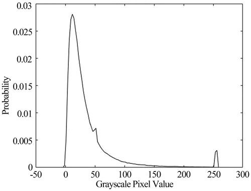
According to the statistical results of the grayscale probability map and the backscattering mechanism of electromagnetic waves of InSAR imaging, when the surface of an object is smooth and nearly perpendicular to the radar beam, the surface of the object can reflect most of the energy of the radar electromagnetic wave to the receiving antenna for the radar. As a result, high scattering feature points appear in the InSAR image, which may contain moving vehicles, glass with changing angles, moored boats, or other targets with high backward scattering coefficients. The accuracy of the image registration is disturbed by the uncertainty introduced by these ultra-high scattering feature points, which usually have pixel values close to 255 in the InSAR greyscale maps, and are commonly found in the range of values between 250 and 255. To ensure the accuracy of image registration, such features should be excluded. Areas with high surface coverage, such as forests and farmlands (in crop growing sea-son), have a low signal-to-noise ratio and serious noise interference in InSAR images due to their low microwave backscattering rate. In contrast, areas with smooth surfaces, such as rivers, lakes and other bodies of water, have reflected signals that are difficult to be captured by the receiving antenna when the angle of incidence of the InSAR electromagnetic wave is greater than 20 degrees. Therefore, these surfaces appear as black areas with low pixel values in the InSAR image. Observation areas such as forests, farmlands, rivers, lakes, etc., are mapped to InSAR grey scale images with pixel values generally within the interval [0, 50]. For objects with distinct geometric features, such as houses, roads, bridges and other objects, they do not change easily over time and have distinct light and dark differences from surrounding objects. Feature points selected at the corner locations of these objects are also easy to match, and such objects have more pronounced texture features and have pixel values generally exceeding 50 in the InSAR greyscale maps.

In order to ensure that image texture information with high contrast and distinctive features is extracted and to obtain stable image features that do not change over time and other factors, it is necessary to enhance the image contrast and to exclude those portions with grey scale pixel values close to 255 and lower than 50, retaining the remaining image grey scale information. In this way, we can extract the DTTM that can accurately reflect the stable features of the image. The steps are as follows:

1. Based on the above principles and statistical analysis, we determine the range of grayscale pixel values [a, b] for extracting DTTI. We take the pixel points whose input grayscale image pixel values within [a, b], then calculate their normalized pixel values and perform a linear transformation. (1) $$I=\{\begin{array}{cc}I,\hfill & a\le I\le b\hfill \\ 0,\hfill & \mathit{\text{else}}\hfill \end{array},$$(1) (2) $$J={\left(\frac{I-a}{b-a}\right)}^{\gamma },$$(2) Where $I$ is the pixel value of the input grayscale image. $\gamma$ is the nonlinear transformation exponent. In this paper, we perform a linear transformation for the images, taking $\gamma =1.$ $J$ is the pixel value of the transformed image.

2. $J$ is Standardized and scaled into the range [m, n], obtaining the pixel value $\mathit{\text{Km}}.$ (3) $$\mathit{\text{Km}}=J\times (m-n)+n,$$(3) Where [m, n] represents the range of values for the normalization of the input image grayscale values. This paper performs sharpening processing for the images, its value is [0, 1].

3. The sharpened pixel value $\mathit{\text{Km}}$ is transformed into a grayscale to get the image after contrast adjustment.

2.2. Generating DTTM

For feature-based image registration method, the accurate extraction of matching feature point pairs at the corresponding positions of two images is the first and crucial step. It directly determines the final registration accuracy. The classical SIFT algorithm is often used to identify and describe local features in images. It can locate important points on various scales and determine their orientation features. However, not all feature points extracted by the SIFT algorithm can be used for image registration. Therefore, a guiding strategy is needed to select the prominent feature points that meet the registration requirements. Here we propose a guiding strategy for the screening of SIFT feature points based on DTTM.

DTTM is a dot trace texture map that can display the contour information of high pixel quality objects in an image. It can display the boundary information of high contrast and prominent texture features in the image. The ability of DTTM to cover most of the high-quality information is an important indicator for evaluating the quality of image point trace texture information.

According to the Persistent Scatterer InSAR (PS-InSAR) principle, feature points are preferentially chosen at prominent locations where the image coherence is high and pixel values differ significantly from those of other nearby points. They are usually the corner points and edge points of a particular geometrical shape, or bright points in dark areas and dark points in bright areas. As a result, before screening the feature points, we first identify the prominent areas suitable for feature point screening. The algorithm of generating DTTM is as follows:

1. For an N*N pixels image, k pixels points $\alpha (x_i,y_i)$ (i = 1……k) are randomly selected. Where $(x_i,y_i)$ is the horizontal and vertical coordinates of the ith pixel point.

2. We define an updated matrix $R$ for storing the pixel points to be traversed in this cycle and a ergodic matrix $\mathit{\text{Er}}$ for cumulatively storing the coordinates of the pixel points which have been traversed. Then k pixel points $\alpha (x_i,y_i)$ are added to $R$ and $\mathit{\text{Er}}.$

3. A window of m*m pixels centered on the pixel points is created in $R.$ It is calculated that the magnitude of the gradient difference $D_i$ between pixel point $\alpha (x_i,y_i)$ and other pixel points $\alpha (x_{i\pm j},y_{i\pm j})$ in the neighborhood within the window. Where $0<j\le (m-1)/2.$ (4) $$D_i=\alpha (x_i,y_i)-\alpha (x_{i\pm j},y_{i\pm j}),$$(4)

4. Determining whether the gradient difference corresponding to point $\alpha (x_i,y_i)$ satisfies the condition $D_i>T_1.$ And if so, we assign this point to the DTTI matrix $W_i.$ Where $T_1$ is the pixel gradient difference threshold. Its value is determined by the level of detail of the desired texture information. The more detailed the texture information desired, the smaller $T_1$ is, and vice versa. Its maximum value is the maximum difference between pixels, and the minimum value is zero.

5. Determining whether the gradient difference between the neighboring pixel points $\alpha (x_{i\pm j},y_{i\pm j})$ within the m*m window that meet the conditions of step 4 and their adjacent pixel points $A(x_i,y_i)$ meets the discrimination condition $G_i\mathrm{<}{T}_2.$ Then the satisfied $A(x_i,y_i)$ is stored in the $F_i$ matrix. (5) $$G_i=\alpha (x_{i\pm j},y_{i\pm j})-A(x_i,y_i),$$(5) $T_2$ is determined by the level of detail of the desired texture information. It differs from $T_1$ in that more detailed the texture information desired, the bigger $T_2$ is, and vice versa.

6. Determining whether all the pixel points in $R$ have been traversed. If all the pixel points have been traversed, $R$ is cleared up.

7. Determining whether the pixel points in the $F_i$ are within $\mathit{\text{Er}}.$ If not, $A(x_i,y_i)$ is added into $R$ and $\mathit{\text{Er}},$ then connecting $A(x_i,y_i)$ to $\alpha (x_i,y_i)$ and removing the pixel point from $F_i.$

8. Determining whether $R$ is empty. If not, turn to step 3) and repeat until $R$ is empty. Otherwise, we end the operation.

The location information extracted using generating DTTM can be used to guide the screening of feature points, which named DTTI. The image composed of the DTTI and its connection relationships is called the DTTM.

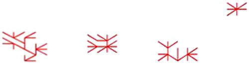
The isolated pixel point is difficult to represent the image features. Therefore, when generating DTTM, it is necessary to eliminate the isolated pixel points to prevent the generation of a dot trace texture as in Figure 2. The specific method is to set the maximum number of connecting lines between a pixel point in DTTM and other pixel points in the neighborhood to $r.$ If the number of connecting lines is greater than $r,$ this pixel point and the connecting lines between it and other pixel points are removed within the DTTM. Where the value of $r$ is determined by the size of the pixel window $m$ that is set when generating the DTTM, $r\le m^2-1.$

Figure 2. The bad DTTM.

The two most important parameters affecting the quality of the produced DTTM are $T_1$ and $T_2.$

To make the DTTI more detailed and to obtain more data in the DTTI matrix $W_i,$ it is necessary to reduce $T_1$ and increase $T_2.$ But if the value of $T_2$ is too large, it will generate too many dot traces textures, as shown in Figure 2. This will produce the a bad DTTM of the image. At the same time, if the value of $T_2$ is too large, it may mistake the noise in the image for DTTI. This is not suitable for guiding SIFT feature screening.

2.3. DTTI-SIFT registration algorithm

In this section, we propose an interferometric image registration algorithm combining DTTI and SIFT (DTTI-SIFT) to improve the registration accuracy and efficiency for SIFT feature points. In the process of generating DTTM, DTTI is extracted that can express the contour information of prominent positions in the image. It contains texture information with high contrast and prominent features, and obtains stable image features that do not change with time or other factors. DTTI is a matrix containing pixel position information, which can be used to guide the screening of image feature points. The DTTI-SIFT algorithm uses DTTI to guide SIFT feature screening. It retains SIFT feature points in the image that are consistent with the DTTI coordinate positions for image registration and eliminates the remaining feature points. The specific steps of the algorithm are as follows:

1. The classical SIFT algorithm is used to extract the feature points of the two interferometric images, and the feature vectors containing the coordinates of the feature points, the direction angle and the scale information are obtained.

2. The feature points are matched by calculating the feature point correlation coefficient and according to a set correlation threshold, and homonymous feature points are generated. Then, we use the RANSAC (Misra et al. 2021; 2023; 2024) method to remove outliers. Referring to the calculation method of the correlation coefficient of the two images, the correlation coefficient for the two feature points can be expressed as: (6) $$\gamma (s,z)=\frac{X(s,z)}{Y(s,z)},$$(6) (7) $$X=P_1{P}_2^T,$$(7) (8) $$Y=\sqrt{\sum _{j=1}^{128}{P}_1{(i,j)}^2{\left(\sum _{j=1}^{128}{P}_2{(i,j)}^2\right)}^T},$$(8) Where $\gamma (s,z)$ is the correlation coefficient of description vector between the $s$th feature point of the master image and the $\mathrm{z}$th feature point of the slave image. $P_1$ and $P_2$ are the feature point description matrices of the master and slave images respectively (each row corresponds to a 128-dimensional feature point description vector). $P_1(i,j)$ and $P_2(i,j)$ are the $j$th ($1\le j\le 128$) dimensional features of the $i$th feature point of the master and slave images respectively. The maximum value on both the rows and columns of $\gamma$ is retrieved. When it is the maximum value on the row and column at the same time and is greater than the threshold value, the sth feature point of the master image and the $\mathrm{z}$th feature point of the slave image corresponding to $\gamma (s,z)$ are the matched feature points pairs. The threshold value of the correlation coefficient depends on the specific conditions of the SIFT feature points. Given the global registration accuracy and running time of the algorithm, after many experimental tests, the threshold value of the correlation coefficient is set to 0.9 in this study.

3. The synonym feature point pair is screened based on the DTTM. The DTTI matrix $W_i$ generated in Section 2.2 and the feature vectors of all synonym SIFT feature points are traversed to find the points where the position coordinates of the feature points are consistent with the DTTI. The matrix $C_{\mathit{\text{point}}}$ is defined for storing the coordinates of the screened feature points. If the relationship between the coordinates $(x_1,y_1)$ of a point in the DTTM and the coordinates $(x_2,y_2)$ of the SIFT feature points satisfies the following in (9), the SIFT feature point should be retained. (9) $$\{\begin{array}{cc}(x_2,y_2)\in C_{\mathit{\text{point}}},\hfill & x_1=x_2\&y_1=y_2\hfill \\ (x_2,y_2)\notin C_{\mathit{\text{point}}},\hfill & \mathit{\text{else}}\hfill \end{array},$$(9)

4. After screening by the above methods, many pairs of feature points are still generally retained in the experiment. So further screening is needed. The actual situation of satellite platform operation and the principle of InSAR imaging show that the directions of images for the same satellite are basically same, even though there are deformations in the them (Dalla Torre et al. 2003; Wang et al. 2011). So, if the directional relationship between a pair of synonym feature point pair relative to other synonym feature point pair has significantly different, it is considered to be incorrectly matched. Assuming that the coordinates of a pair of synonym feature points are $(u_1,v_1)$ and $(u_2,v_2).$ The slope $K_{\mathit{\text{ab}}}$ of the line connecting the two points is: (10) $$K_{\mathit{\text{ab}}}=\frac{v_2-v_1}{u_2-u_1},$$(10)

When the slope $K_{\mathit{\text{ab}}}$ lies within ($\overline{K_{\mathit{\text{ab}}}}-\delta ,$ $\overline{K_{\mathit{\text{ab}}}}+\delta$), it is considered that the synonym feature point pair can be used for the final image registration. At the same time, the pairs of synonym feature points satisfying the above condition is put into the matrix $M_{\mathit{\text{pairs}}}.$ (11) $$\{\begin{array}{cc}(u_1,v_1),(u_2,v_2)\in M_{\mathit{\text{pairs}}},\hfill & \overline{K_{\mathit{\text{ab}}}}-\delta \le K_{\mathit{\text{ab}}}\le \overline{K_{\mathit{\text{ab}}}}+\delta \hfill \\ (u_1,v_1),(u_2,v_2)\notin M_{\mathit{\text{pairs}}},\hfill & \mathit{\text{else}}\hfill \end{array},$$(11) Where $\overline{K_{\mathit{\text{ab}}}}$ is the mean value of the slope for the connection of pairs of synonym feature points. And in the proposed algorithm of this paper, $\delta$ is set to 0.02 by repeated experimental debugging.

2.4. Filtering algorithm based on semantic segmentation

The noise can reduce the quality of the interferometric phase diagram, and error diffusion from low-quality interferometric phase regions will reduce the signal-to-noise ratio of high-quality interferometric phase regions during filtering. To improve the filtering results of the interferometric phase diagram, and reduce the impact of low-quality interferometric phase regions on high-quality interferometric phase regions, we proposed a filtering algorithm based on semantic segmentation. First, the interferometric phase diagram is performed semantic segmentation based on the correlation coefficients between images after registration. For the high-quality interferometric phase regions after segmentation, we first use the two-dimensional frequency domain rotational symmetric Gaussian Laplace filtering method for filtering, and then use the wavelet domain filtering method for filtering. For the low-quality interferometric phase regions, we use average filter to smooth out noise. Another purpose of this algorithm is to filter out phase noise as much as possible and smooth out edge details corresponding to significant changes in terrain features as little as possible. The specific steps of this algorithm are as follows:

1. The two registered images are evenly divided into several $H$*$H$ sub-images respectively, and the correlation coefficient $\mathit{\text{CC}}$ of each pair of the corresponding sub-images is calculated. Where the size $H$ of the sub-images is determined by the magnitude of the difference among local correlation coefficient for the registered images.

2. Taking the correlation coefficient $\mathit{\text{CC}}$ as the semantic of the images. The interferometric phase diagram is segmented into several regions by setting a segmentation threshold $r_{\mathrm{\text{min}}}.$ Where $r_{\mathrm{\text{min}}}$ is determined according to the probability distribution of the correlation coefficient for the images. And in the proposed algorithm, $r_{\mathrm{\text{min}}}$ takes the correlation coefficient value with the highest probability.

3. The sub-images of interferometric phase diagram with correlation coefficients less than $r_{\mathrm{\text{min}}}$ are classified as class ${\mathit{\text{Area}}}_{\mathrm{\text{min}}}.$ Whereas those with correlation coefficients more than $r_{\mathrm{\text{min}}}$ are classified as class ${\mathit{\text{Area}}}_{\mathrm{\text{max}}}.$ For the sub-images belong to ${\mathit{\text{Area}}}_{\mathrm{\text{min}}},$ the mean filtering algorithm is used to smooth the phase noise. And for the sub-images belong to ${\mathit{\text{Area}}}_{\mathrm{\text{max}}},$ the algorithm first two-dimensional frequency domain rotationally symmetric Gaussian Laplacian filtering followed by wavelet domain filtering is adopted to remove and smooth the noise.

4. For the problem of discontinuity in the boundary pixels of different classes for sub-regions in the interferometric phase diagram after the using the above filtering method, a 3*3 mean filtering is used for smoothing to obtain the final interferometric phase diagram.

3. Experiment and result analysis

In this section, we describe the experiment in detail and analyze the results. Firstly, we introduce the data used in the experiment. In addition, we will validate the performance of the proposed method on several items: 1) We compared our algorithm with the other four algorithms and observe the performance of the algorithm using the interferometric phase diagram; 2) We compared the overall registration performance of the five algorithms using five commonly used evaluation metrics; 3) We statistically compared the performance of the five algorithms on local registration through the method of image chunking statistics. After that, the performance of our proposed filtering algorithms is verified by interferometric phase diagram.

3.1. Experimental data

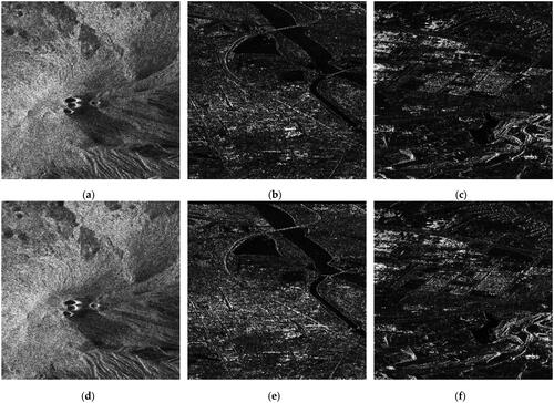
The experimental data contains three groups. The first group is the ERS1/2 images acquired during two passes through the Etna volcanic area on October9 and 10, 1994. Their azimuthal resolution is 40 m, and their range resolution is 25 m. In this research, an area of 600*600 pixels from the images is selected for the experiment. And the amplitude maps of the two complex images, as shown in Figure 3a, d. The second group is the two images acquired by the Sentinel-1 satellite (abbr. Sentinel-1) in the Inner Mongolia section of the Yellow River basin on August 6, 2022, and July 25, 2022. And the third group is the two images acquired by the Sentinel-1 satellite in the Inner Mongolia section of the Yellow River basin on May 9, 2023, and June 2, 2023. Their azimuthal resolution is 14.1 m, and their range resolution is 2.3 m. In this research, areas of 800*800 pixels are selected from the images for experimentation. The amplitude maps of two complex images for the second group are shown in Figure 3b, e. And the amplitude maps for the third group of the two complex images are shown in Figure 3c, f. The data in the preceding three groups are all SLC data and the polarization method is VV.

Figure 3. Amplitude map of the image to be registered: (a, d) the two amplitude maps for the first group of images respectively; (b, e) the two amplitude maps for the second group of images respectively; (c, f) the two amplitude maps for the third group of images respectively.

3.2. Images registration experiments and results analysis

First, the grayscale probability maps of the three images to be registered as shown in Figure 3a, b, c are drawn, as shown in Figure 4. As shown in Figure 4, the probability of the ERS1/2 images reaches its maximum value at a grayscale pixel value of around 80, and a probability mutation occurs at a grayscale pixel value of around 120. The probability of the two Sentinel-1 images reaches its maximum value at a grayscale pixel value of around 10, a probability mutation occurs at a grayscale pixel value of around 50. In order to extract DTTI that can clearly express the image without increasing the computational complexity, according to Figure 4 and the method in Section 2.1, the pixel value range for adjusting the gray level is determined to be [0.25, 0.27]. Also, the method in Section 2.1 is applied to sharpen the images to be registered. The sharpened grayscale images are shown in Figure 5.

Figure 4. Grayscale probability map: (a) the grayscale probability map of Figure 3a; (b) the grayscale probability map of Figure 3b; (c) the grayscale probability map of Figure 3c.

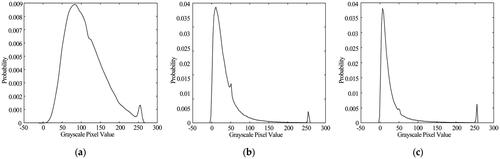
Figure 5. Images after sharpening grayscale images: (a) images after sharpening grayscale images of Figure 3a; (b) images after sharpening grayscale images of Figure 3b; (c) images after sharpening grayscale images of Figure 3c.

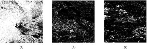
Second, the DTTM was produced using the method discussed in Section 2.2. In this paper, after repeated tests, we set the window size m = 3, the pixel gradient difference thresholds $T_1$=80 and $T_2$=100. And the maximum number $r$ of connected lines between a pixel in DTTM and other pixels in the neighborhood is 4. The obtained DTTMs are shown in Figure 6. At the same time, the DTTI matrix $W_i$ can be generated. Then, we use the classical SIFT algorithm to extract the feature points of the three groups of InSAR images respectively, as shown in Figure 3. Furthermore, the feature points are screened according to the DTTI matrix $W_i.$ And the feature point pairs with a slope of the connecting line greater than the threshold are eliminated. The transformation matrix between the master image and the slave image is calculated by the affine transformation method based on the final reserved feature point pairs. Next, the position coordinates for the pixel points of the slave image are calculated based on the transformation matrix. The slave image is interpolated 10 times by the bilinear interpolation method and then resampled. The values of pixels accurately registered with the master image are extracted to construct a new image, which is the accurate registration result of the slave image. The complex conjugate of the registered slave image is multiplied by the master image to produce the phase diagram shown in Figure 7d, e, f.

Figure 6. DTTM of three images: (a) the DTTM of Figure 3a; (b) the DTTM of Figure 3b; (c) the DTTM of Figure 3c.

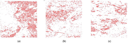
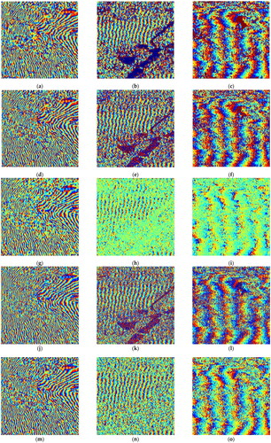
Figure 7. Interferometric phase diagrams generated after registered of three groups of images using four registration algorithms: (a, b, c) the interferometric phase diagrams generated using the classical SIFT algorithm for the three groups of images respectively; (d, e, f) the interferometric phase diagrams generated using the DTTI-SIFT algorithm for the three groups of images respectively; (g, h, i) the interferometric phase diagrams generated using the KAZE-SAR algorithm for three groups of images respectively; (j, k, l) the interferometric phase diagrams generated using the MU-Net algorithm for three groups of images respectively; (m, n, o) the interferometric phase diagrams generated using the ORB algorithm for three groups of images respectively.

To demonstrate the advantages of the proposed algorithm, the same three groups of experimental images were accurately registered using the classical SIFT algorithm, the ORB algorithm (Rublee et al. 2011; Misra et al. 2021, 2022), the KAZE-SAR algorithm and the MU-Net algorithm. The obtained interferometric phase diagrams are shown in Figure 7 (a), (b), (c), (g–o). It can be seen from Figure 7 that the definition and the number of interferometric fringes in the interferometric phase diagram generated after registration with the DTTI-SIFT algorithm are better than those with the classical SIFT algorithm, the ORB algorithm, the KAZE-SAR algorithm and the MU-Net algorithm.

To compare the registration performance of the above five algorithms and verify the advantages of the proposed DTTI-SIFT algorithm, we carried out the statistical analysis of the registration experimental results using five common evaluation indicators. They are correlation coefficient (CC), mean square error (MSE), normalized correlation coefficient (NCC), mutual information (MI), and normalized mutual information (NMI). The results of the statistical analysis are shown in Tables 1-3.

Table 1. Comparison of evaluation indicators for the registration performance of the first group images.

	SIFT	ORB	KAZE-SAR	MU-Net	DTTI-SIFT
CC	0.8498	0.7690	0.7806	0.7820	0.8542
MSE	6166.3	9493.7	9051.4	8995.2	5992.5
NCC	0.5086	0.2413	0.2708	0.2761	0.5993
MI	0.5288	0.3855	0.3982	0.4006	0.5466
NMI	1.034	1.0021	1.0254	1.0255	1.0352

Table 2. Comparison of evaluation indicators for the registration performance of the second group images.

	SIFT	ORB	KAZE-SAR	MU-Net	DTTI-SIFT
CC	0.7973	0.7267	0.7323	0.7537	0.8207
MSE	20.1115	26.8327	26.2855	24.3145	17.7824
NCC	0.3434	0.1226	0.1397	0.2055	0.4219
MI	0.0924	0.0162	0.0189	0.0352	0.1423
NMI	1.0124	1.0021	1.0025	1.0047	1.0192

Table 3. Comparison of evaluation indicators for the registration performance of the third group images.

	SIFT	ORB	KAZE-SAR	MU-Net	DTTI-SIFT
CC	0.8111	0.6945	0.7358	0.7328	0.8389
MSE	15.2188	24.6538	26.0748	21.524	12.9810
NCC	0.4740	0.1502	0.1438	0.2595	0.5515
MI	0.1586	0.0166	0.0200	0.0463	0.2248
NMI	1.0223	1.0023	1.0027	1.0064	1.0319

From Tables 1-3, it shows that the three group images registered with the DTTI-SIFT algorithm outperformed the classical SIFT algorithm, the ORB algorithm, the KAZE-SAR algorithm and the MU-Net algorithm in five evaluation metrics: CC, MSE, NCC, MI and NMI. The results of the registration using the DTTI-SIFT algorithm outperformed the other four algorithms in overall registration performance, pixel value difference and probabilistic correlation for the three group images. In the experiment, the evaluation index of the SIFT algorithm after registration was better than that of the MU-Net algorithm because the MU-Net algorithm is suitable for the registration of multimodal image pairs with large deformation, while the SIFT algorithm has a better registration effect in the registration of images with obvious features and little deformation.

To illustrate the improvement in local registration performance of the DTTI-SIFT algorithm compared to the other four algorithms, the registered image pairs were uniformly divided into sub-images with 2*2 pixels. And the correlation coefficients of the sub-image pairs are calculated and counted for comparison with the classical SIFT algorithm, the ORB algorithm, the KAZE-SAR algorithm and the MU-Net algorithm, as shown in Figure 8.

Figure 8. Distribution map of the correlation coefficient for the Sub-blocks of the three groups of images: (a, b, c) the distributions of the correlation coefficient for each Sub-block of the three groups of images after registration using the classical SIFT algorithm respectively; (d, e, f) the distributions of the correlation coefficient for each Sub-block of the three groups of images after registration using the DTTI-SIFT algorithm respectively; (g, h, i) the distributions of the correlation coefficient for each Sub-block of the three groups of images after registration using the KAZE-SAR algorithm respectively; (j, k, l) the distributions of the correlation coefficient for each Sub-block of the three groups of images after registration using the MU-Net algorithm respectively; (m, n, o) the distributions of the correlation coefficient for each Sub-block of the three groups of images after registration using the ORB algorithm respectively.

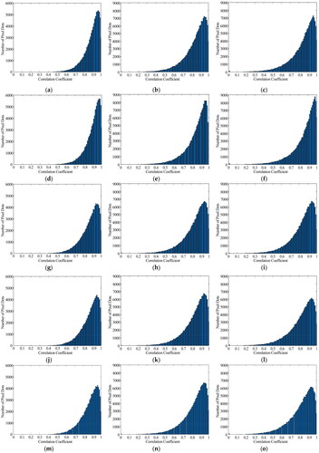
The statistics results of Figure 8 (a), (d), (g), (j), (m) show that the number of sub-image pairs with correlation coefficients between 0.96 and 0.98 is the highest, accounting for 18.879% of the total when using the classical SIFT algorithm. When using the ORB algorithm, the number of sub-image pairs with correlation coefficients between 0.94 and 0.96 is the highest, accounting for 14.948% of the total. When using the KAZE-SAR algorithm, the number of sub-image pairs with correlation coefficients between 0.94 and 0.96 is the highest, accounting for 15.310% of the total. And when using the MU-Net algorithm, the number of sub-image pairs with correlation coefficients between 0.94 and 0.96 is the highest, accounting for 15.256% of the total. While using the DTTI-SIFT algorithm, the number of sub-image pairs with correlation coefficients between 0.96 and 0.98 is the highest, accounting for 20.065% of the total. Moreover, using the classical SIFT algorithm, the ORB algorithm, the KAZE-SAR algorithm, the MU-Net algorithm and the DTTI-SIFT algorithm for the registration of the three groups of images, the correlation coefficients of the subblocks after registration that are greater than 0.8 respectively account for 84.944%, 76.524%, 77.315%, 77.385% and 86.527% of the total; And the correlation coefficients of the subblocks after registration that are less than 0.6 respectively account for 1.182%, 2.208%, 2.253%, 2.257% and 0.988% of the total.

The statistics results of Figure 8 (b), (e), (h), (k), (n) show that the number of sub-image pairs with correlation coefficients between 0.95 and 0.97 is the highest, accounting for 13.748% of the total when using the classical SIFT algorithm. When using the ORB algorithm, the number of sub-image pairs with correlation coefficients between 0.94 and 0.96 is the highest, accounting for 12.799% of the total. When using the KAZE-SAR algorithm, the number of sub-image pairs with correlation coefficients between 0.94 and 0.96 is the highest, accounting for 12.774% of the total. And when using the MU-Net algorithm, the number of sub-image pairs with correlation coefficients between 0.94 and 0.96 is the highest, accounting for 12.786% of the total. While using the DTTI-SIFT algorithm, the number of sub-image pairs with correlation coefficients between 0.96 and 0.98 is the highest, accounting for 15.715% of the total. Moreover, using the classical SIFT algorithm, the ORB algorithm, the KAZE-SAR algorithm, the MU-Net algorithm and the DTTI-SIFT algorithm for the registration of the three groups of images, the correlation coefficients of the subblocks after registration that are greater than 0.8 respectively account for 71.517%, 68.296%, 68.650%, 68.540% and 74.892% of the total; And the correlation coefficients of the subblocks after registration that are less than 0.6 respectively account for 5.618%, 6.570%, 6.452%, 6.402% and 5.008% of the total.

The statistics results of Figure 8 (c), (f), (i), (l), (o) show that the number of sub-image pairs with correlation coefficients between 0.95 and 0.97 is the highest, accounting for 13.668% of the total when using the classical SIFT algorithm. When using the ORB algorithm, the number of sub-image pairs with correlation coefficients between 0.93 and 0.95 is the highest, accounting for 11.771% of the total. When using the KAZE-SAR algorithm, the number of sub-image pairs with correlation coefficients between 0.94 and 0.96 is the highest, accounting for 12.786% of the total. And when using the MU-Net algorithm, the number of sub-image pairs with correlation coefficients between 0.93 and 0.97 is the highest, accounting for 11.669% of the total. While using the DTTI-SIFT algorithm, the number of sub-image pairs with correlation coefficients between 0.97 and 0.99 is the highest, accounting for 16.249% of the total. Moreover, using the classical SIFT algorithm, the ORB algorithm, the KAZE-SAR algorithm, the MU-Net algorithm and the DTTI-SIFT algorithm for the registration of the three groups of images, the correlation coefficients of the subblocks after registration that are greater than 0.8 respectively account for 69.887%, 64.436%, 68.540%, 64.311% and 74.543% of the total; And the correlation coefficients of the subblocks after registration that are less than 0.6 respectively account for 6.985%, 8.356%, 6.402%, 8.292% and 5.824% of the total.

From the above statistical analysis, it can be seen that the DTTI-SIFT algorithm, which uses DTTI to guide SIFT feature point screening, can not only improve the global performance for image registration but also the local correlation, compared to the classical SIFT algorithm, the ORB algorithm, the KAZE-SAR algorithm and the MU-Net algorithm.

Finally, the filtering algorithm based on the semantic segmentation proposed above is used to deal with the interferometric phase diagram obtained after registration. First, the image pairs after registration are uniformly segmented into sub-blocks of 6*6 pixels, and then the correlation coefficient of the sub-image pairs is calculated. Based on statistical analysis, the correlation coefficient CC = 0.65 is used as the threshold. Second, the interferometric phase diagrams shown in Figure 7 (d), (e), (f) are performed semantic segmentation according to the correlation coefficient of the registered images and its threshold. For the high-coherence and low-coherence sub-images of the interferometric phase diagrams, the proposed algorithm in Section 2.4 is employed to finish the interferometric phase filtering respectively. And the interferometric phase diagrams after filtering and removing the flat earth effect are shown in Figure 9 (a), (b), (c).

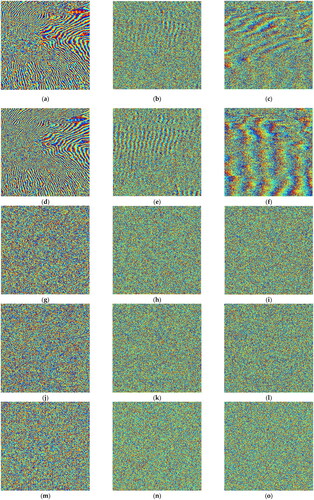
Figure 9. Interferometric phase diagrams of three groups of images after registration with the DTTI-SIFT algorithm: (a, b, c) the interferometric phase diagram obtained by filtering the three groups of images using the proposed algorithm; (d, e, f) the interferometric phase diagram obtained by filtering the three groups of images using the filtering method combining two-dimensional frequency domain filtering and wavelet filtering; (g, h, i) the interferometric phase diagram obtained by filtering the three groups of images using the adaptive direction filtering algorithm based on optimal integration; (j, k, l) the interferometric phase diagram obtained by filtering the three groups of images using the two-dimensional frequency domain filtering algorithm; (m, n, o) the interferometric phase diagram obtained by filtering the three groups of images using the wavelet filtering algorithm.

In order to prove the superiority of the proposed filtering algorithm based on semantic segmentation, it is compared with two algorithms without semantic segmentation. First, the filtering method that combines two-dimensional frequency domain filtering and wavelet filtering without semantic segmentation is used to filter the whole interferometric phase diagram obtained after the registration of the DTTI-SIFT algorithm. The interferometric phase diagrams after filtering and removing the flat earth effect are shown in Figure 9 (d–f). Second, the adaptive direction filtering algorithm based on optimal integration (Jiang et al. 2019) is used to filter the whole interferometric phase diagram obtained after the registration of the DTTI-SIFT algorithm. The interferometric phase diagrams after filtering and removing the flat earth effect are shown in Figure 9 (g–i).

In order to demonstrate the influence of two-dimensional frequency domain filtering and wavelet filtering in the proposed filtering algorithm based on semantic segmentation, ablation experiments were conducted on them. The entire interferometric phase diagram obtained after registration with the DTTI-SIFT algorithm was filtered using two-dimensional frequency domain filtering and wavelet filtering, respectively. The filtered and ground effect removed interferometric phase diagrams are shown in Figure 9 (j–l) and Figure 9 (m–o), respectively.

From Figure 9, it can be seen that the proposed filtering algorithm in this paper can improve the definition of the interferometric fringes. It can restrain the spread of phase errors from low-quality phase regions to the high-quality ones. And there are fewer noise patches in the interferometric phase diagram after filtered. The edge information is basically retained, not smoothed significantly. The optimization effect of the interferometric phase diagram is most noticeable in low-coherence regions such as rivers and lakes. Overall, the proposed filtering algorithm is better than the filtering method combining two-dimensional frequency domain filtering and wavelet filtering, the adaptive direction filtering algorithm based on optimal integration, the two-dimensional frequency domain filtering algorithm, and the wavelet filtering algorithm.

4. Conclusion and discussion

In this paper, we propose an interferometric phase diagram generation method based on DTTI and semantic segmentation of correlation coefficients. It contains two stages. The first is an interferometric image registration algorithm which extracting SIFT features based on dot trace texture information. Before screening the SIFT feature points, DTTI is extracted based on the sharpened grayscale image, which reflects the edges, contours and structural features of the image. Then the SIFT feature points screening is performed with guidance from DTTI. In this way, the number of SIFT feature points used for registration is reduced. Most importantly, this can also improve the stability and accuracy of the SIFT algorithm and obtain the SIFT feature points located at prominent positions in the image for accurate image registration. The experimental results and their statistical analysis show that the proposed registration algorithm can be used for the accurate registration of complex InSAR images. Its local correlations and the global evaluation indicators CC, MSE, NCC, MI, and NMI are better than the classical SIFT algorithm, the KAZE-SAR algorithm and the MU-Net algorithm. The second is a filtering algorithm based on the semantic segmentation of correlation coefficients. The different filtering methods are used for sub-regions of the interferometric phase diagram with different correlations. The experiments results show that the proposed filtering algorithm can improve the quality of the interferometric fringes, restrain the spread of phase errors, and retain the edge information. Its effectiveness are better than the filtering method combining two-dimensional frequency domain filtering and wavelet filtering, the adaptive direction filtering algorithm based on optimal integration, the two-dimensional frequency domain filtering algorithm, and the wavelet filtering algorithm.

Although the proposed method can produce high-quality interferometric phase diagram for the images of InSAR, the experimental images used in this paper covers a small area. For the registration of InSAR images in large-scale complex geographical environments, the signal-to-noise ratio of images for different areas will vary because of the different backward scattering characteristics and coherence. If the proposed DTTI-SIFT algorithm is used for the DTTI extraction in them, the results may contain many errors and noises. This may lead to incorrect screening of SIFT feature points. It is the focus of our next research.

Acknowledgments

Authors would like to show their gratitude to the editors and the anonymous reviewers for their insightful comments.

Data availability statement

The Sentinel-1 datasets were freely provided by Copernicus Open Access Hub, https://scihub.copernicus.eu/dhus/#/home.

Disclosure statement

The authors declare no conflict of interest.

Additional information

Funding

This research was funded by Natural Science Foundation of Inner Mongolia Autonomous Region (2022QN06005), the Basic Scientific Research Funds for Colleges and Universities directly under the Inner Mongolia Autonomous Region (JY20220225), the Scientific Research Start-up Funds of Inner Mongolia University of Technology (DC2200000948), and the Open Foundation of State key Laboratory of Networking and Switching Technology (Beijing University of Posts and Telecommunications) (SKLNST-2021-1-19).

References

- Chen B, Li Z, Zhang C, Ding M, Zhu W, Zhang S, Han B, Du J, Cao Y, Zhang C, et al. 2022. Wide area detection and distribution characteristics of landslides along Sichuan expressways. Remote Sens. 14:3431–3452.
- Dalla Torre A, Van Leeuwen F. 2003. A detailed analysis of the operational orbit of the hipparcos satellite. Space Sci Rev. 108(3):451–470. doi: 10.1023/A:1026215716256.
- Dellinger F, Delon J, Gousseau Y, Michel J, Tupin F. 2015. SAR-SIFT: a SIFT-like algorithm for SAR images. IEEE Trans Geosci Remote Sens. 53:453–466.
- Fan R, Hou B, Liu J, Yang J, Hong Z. 2020. Registration of multiresolution remote sensing images based on L2-siamese model. IEEE J Sel Top Appl Earth Obs Remote Sens. 14:237–248.
- Goldstein RM, Werner CL. 1998. Radar interferogram filtering for geophysical applications. Geophys Res Lett. 25(21):4035–4038. doi: 10.1029/1998GL900033.
- Jiang H, Ma Y, Su Z, Dai M, Yang F, He X. 2019. Speckle-interferometric phase fringe patterns de-noising by using fringes’ direction and curvature. Opt. Lasers Eng. 119:30–36.
- Li T, Chen KS, Lee JS. 2020. Enhanced interferometric phase noise filtering of the refined InSAR filter. IEEE Geosci Remote Sens Lett. 17:1528–1532.
- Lowe DG. 2004. Distinctive Image Features from Scale-Invariant Keypoints. International Journal of Computer Vision. 60:91–110. 10.1023/B:VISI.0000029664.99615.94.
- Lu Z, Kwoun O, Rykhus R. 2007. Interferometric synthetic aperture radar (InSAR): its past, present and future. Photogramm Eng Rem S. 73:217–221.
- Mao S, Yang J, Gou S, Jiao L, Xiong T, Xiong L. 2021. Multi-scale fused SAR image registration based on deep forest. Remote Sens. 13:2227–2245.
- Men P, Guo H, An J, Li G. 2022. An improved L2Net for repetitive texture image registration with intensity difference heterogeneous SAR images. Remote Sens. 14:2527–2547.
- Misra I, Rohil MK, Moorthi SM, Dhar D. 2021. FIRM: framework for image registration using multistage feature detection and mode-guided motion smoothness keypoint optimization. IEEE Trans Geosci Remote Sens. 60:1–12.
- Misra I, Rohil MK, Moorthi SM, Dhar D. 2022. Feature based remote sensing image registration techniques: a comprehensive and comparative review. Int J Remote Sens. 43(12):4477–4516. doi: 10.1080/01431161.2022.2114112.
- Misra I, Rohil MK, Moorthi SM, Dhar D. 2023. MIRACLE: multi-satellite Island image registration using anisotropic coherence locality enhanced nonlinear diffusion and Mahalanobis distance guided marginalization. Int J Remote Sens. 44(12):3753–3776. doi: 10.1080/01431161.2023.2225713.
- Misra I, Rohil MK, Moorthi SM, Dhar D. 2024. Direct feature extraction and image co-registration of morphological structure from Bayer pattern raw planetary images. Expert Syst Appl. 238:122274. doi: 10.1016/j.eswa.2023.122274.
- Misra I, Rout L, Arya S, Bhateja Y, Moorthi SM, Dhar D. 2021. Phobos image enhancement using unpaired multi-frame acquisitions from Indian Mars Color Camera. Planet Space Sci. 201:105215. doi: 10.1016/j.pss.2021.105215.
- Ni X, Cao C, Ding L, Jiang T, Zhang H, Jia H, Li G, Zhao J, Chen W, Ji W, et al. 2012. A fully automatic registration approach based on contour and SIFT for HJ-1 images. Sci China Earth Sci. 55(10):1679–1687. doi: 10.1007/s11430-012-4455-7.
- Ordóñez Á, Acción Á, Argüello F, Heras DB. 2021. HSI-MSER: hyperspectral image registration algorithm based on MSER and SIFT. IEEE J Sel Top Appl Earth Obs Remote Sens. 14:12061–12072.
- Pourfard M, Hosseinian T, Saeidi R, Motamedi SA, Abdollahifard MJ, Mansoori R, Safabakhsh R. 2022. KAZE-SAR: SAR image registration using KAZE detector and modified SURF descriptor for tackling speckle noise. IEEE Trans Geosci Remote Sens. 60:1–12.
- Reddy BS, Chatterji BN. 1996. An FFT-based technique for translation, rotation, and scale-invariant image registration. IEEE Trans Image Process. 5(8):1266–1271.
- Rublee E, Rabaud V, Konolige K, Bradski G. 2011. ORB: an efficient alternative to SIFT or SURF. In Proceedings of the 2011 International Conference on Computer Vision. 2564–2571. Barcelona, Spain.
- Wang T, Perissin D, Rocca F, Liao MS. 2011. Three Gorges Dam stability monitoring with time-series InSAR image analysis. Sci China Earth Sci. 54(5):720–732. doi: 10.1007/s11430-010-4101-1.
- Xiong X, Jin G, Xu Q, Liu X, Shi Q. 2024. Robust multi-view UAV SAR image registration based on selective correlation of log gradient descriptor. Int J Appl Earth Obs Geoinf. 127:103678. doi: 10.1016/j.jag.2024.103678.
- Xu G, Gao Y, Li J, Xing M. 2020. InSAR phase denoising: a review of current technologies and future directions. IEEE Geosc Rem Sen M. 8:64–82.
- Xu H, Li Z, Li S, Liu W, Li J, Liu A, Li W. 2021. A nonlocal noise reduction method based on fringe frequency compensation for SAR interferogram. IEEE J Sel Top Appl Earth Obs Remote Sens. 14:9756–9767.
- Yague-Martinez N, De Zan F, Prats-Iraola P. 2017. Coregistration of interferometric stacks of sentinel-1 TOPS data. IEEE Geosci Remote Sens Lett. 14:1002–1006.
- Yan Z, Yan H, Wang T. 2021. A fast non-local means filtering method for interferometric phase based on wavelet packet transform. Radio Sci. 56:1–14.
- Yang H, Li X, Zhao L, Chen S. 2019. A novel coarse-to-fine scheme for remote sensing image registration based on SIFT and phase correlation. Remote Sens. 11(15):1833. doi: 10.3390/rs11151833.
- Ye Y, Tag T, Zhu B, Yang C, Li B, Hao S. 2022. A multiscale framework with unsupervised learning for remote sensing image registration. IEEE Trans Geosci Remote Sens. 60:1–15.
- Zhang J, Ma W, Wu Y, Jiao L. 2019. Multimodal remote sensing image registration based on image transfer and local features. IEEE Geosci Remote Sens Lett. 16:1210–1214.
- Zhang H, Ni W, Yan W, Xiang D, Wu J, Yang X, Bian H. 2019. Registration of multimodal remote sensing image based on deep fully convolutional neural network. IEEE J Sel Top Appl Earth Obs Remote Sens. 12:3028–3042.
- Zou W, Li Y, Li Z, Ding X. 2009. Improvement of the accuracy of InSAR image co-registration based on tie points–a review. Sensors. 9(2):1259–1281. doi: 10.3390/s90201259.