Extracting multilane roads from OpenStreetMap through graph convolutional neural network and road mesh relationship analysis

Abstract

Multilane roads in vector data are comprised of parallel line features that represent the same road. The extraction of these features is crucial for updating maps and cartographic generalization. This article addresses previous object-level extraction limitations by introducing a mesh-based method that employs a GCNN model to classify them based on geometric features and proximity relationship. A bidirectional region growing clustering method (BRGC) is designed to cluster the identified multilane road meshes belonging to the same road into groups considering their spatial relationships. The object-level multilane roads are extracted based on the clustering results. Validation using road data from OpenStreetMap in Chengdu and Zhengzhou achieved a classification f1-score >90% for multilane road mesh. Moreover, the object-level multilane detection precision and recall were 88.05% and 92.72% on the Chengdu dataset, and 86.99% and 91.37% on the Zhengzhou dataset, which demonstrates the proposed method effectively extracts multilane roads at the object level, aligning with real-world scenarios and human cognition.

Keywords:

• Cartographic generalization
• road network
• multilane road extraction
• graph convolutional neural network

1. Introduction

With the series of fundamental scale geodatabases gradually being established, the rapid development of urbanization demands a shorter update cycle for existing road network databases. Efficient management of road network data at various scales and hierarchical levels presents a challenge and research hotspot in geodatabase management technology. An essential aspect of effectively addressing this challenge entails automatically identifying the same geographical elements across different datasets and establishing the matching relationships among them. (Tong et al. 2014; Kim et al. 2017; Ali Abbaspour et al. 2018; Chehreghan and Ali Abbaspour 2018). Therefore, the accurate and rapid identification and establishment of matching relationships among the entities with the same names at different scales constitute the foundation for the subsequent updating, integration, and fusion of road data, and are of great significance.

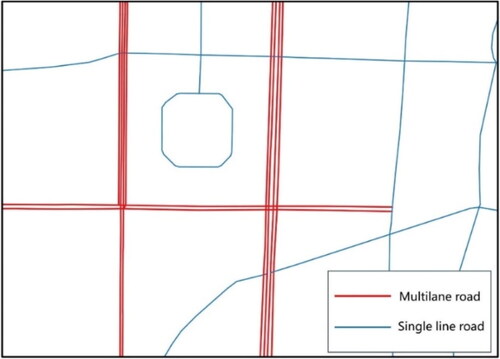
Nevertheless, matching road networks at different scales presents a set of challenges. One specific challenge arises from the transformation of a multilane road into a single or dual lane road as the scale decreases, leading to one-to-many (1:N) or many-to-many (N:M) matching relationships between the same road. Multilane roads are a type of salient road pattern in large-scale vector maps composed of a set of approximately parallel road line segments representing the same road (Li et al. 2014; Wu et al. 2022; Xu et al. 2019), as the red road segments depicts in Figure 1. In different road data with varying scales, when the number of line features forming the same road is different, it is challenging to accurately identify their corresponding relationships by solely relying on existing map matching technology (Guo et al. 2017). By detecting multilane roads, the complex relationships between road segments in different datasets can be simplified into a one-to-one (1:1) relationship, reducing the difficulty of matching process. Accordingly, multilane road extraction is a crucial step in road network matching, and it significantly contributes to the management of multiscale geodatabases. Furthermore, the multilane road extraction also provides valuable information for the cartographic generalization of road networks (Chen et al. 2009; Touya 2010; Zhou and Li 2016; Shoman and Gülgen 2017; Yu et al. 2020), facilitating the determination of the specific set of road segments that require typification (Stefanakis 2015).

Figure 1. Example of multilane roads and single-lane roads.

Within the high level of detail (LoD) datasets, urban arterial roads are commonly organized as multilane roads, considering the physical separator between lanes. These roads play a crucial role in facilitating the movement of people and goods, forming the major pattern of urban transportation and spatial structure (Jiang 2009; Gülgen 2014; Hu et al. 2017; Wang, You, and Wang 2017; Hong and Yao 2019; Mann et al. 2022), which are crucial for many modern application such as geographical analysis (Heinzle et al. 2006; Grigorescu et al. 2022), traffic planning (Li et al. 2019) and location-based service (LBS). However, in most of the common datasets, such as OpenStreetMap (OSM), the multilane attributes might not be stored explicitly in many regions.

Attribute information, such as road names, facilitates the rapid extraction of multilane roads. However, practical applications encounter challenges due to the low quality of road network data, including the absence or inconsistency of attribute information (Li et al. 2014). For instance, a multilane road that maintains spatial continuity may be assigned different names in various administrative regions. To overcome these limitations, resent studies have developed algorithms for the automatic identification of multilane roads from a geometric perspective. These studies have attained a promising recognition accuracy by focusing on linear road segments or polygonal road meshes as identification elements. Nevertheless, these approaches still exhibit areas for improvement. For instance, while recognition results based on road meshes can ascertain whether a road is a multilane road, scant attention has been devoted to extracting independent multilane roads, ie, at the object level, which hold significant implications for subsequent tasks such as cartographic generalization and map matching.

In this study, we propose a novel framework for multilane road detection at the object level. This framework also employs the strategy of classifying road meshes based on shape features. The design of the entire framework is as follows. First, a graph convolutional neural network (GCNN) is introduced to identify the multilane road meshes by considering the geometric features of the meshes and their neighbors. Second, considering the spatial relationships among the meshes of the same single multilane road, a bidirectional region growing clustering (BRGC) method is proposed to cluster the multilane meshes into groups based on their extension and parallel relationships. Finally, the meshes in each group are merged, and the multilane roads are extracted considering the overlap relation between the combined meshes and the road network.

The remainder of this article is organized as follows. Section 1 introduces the related research background and research significance. Section 2 introduces the related studies. Section 3 explains the proposed multilane road extraction framework in detail. Section 4 presents various experiments and discussions about the extraction results. Section 5 summarizes the whole paper and provides an outlook for future research.

2. Related work

2.1. Approaches for extracting multilane roads

Depending on the geometry types of the processed features, the existing methods for multilane road extraction can be categorized into two groups: segment-based methods and mesh-based methods.

The segment-based methods rely on proximity and similarity of geometric features such as distance, orientation, and length of the line features of multilane roads. Thom (2002) identified dual-lane roads by using deflection angle and extension orientation of road segments as constraints. Yang et al. (2011) first determined a set of candidate road segments that can form dual-lane roads based on the buffer analysis, calculated the distances and orientation angles between the road segments in the set to extract dual-lane road segments, and finally merged the dual-lane road segments into dual-lane roads according to the principle of good extensibility. In his article, the Hausdorff distance was used instead of the perpendicular distance between road segments. Based on this process, subsequent studies further refined the algorithmic details to enhance its performance. For instance, improvements have been made in the calculation methods for distances between road segments (Gong et al. 2021; Xing et al. 2018), as well as optimizations in the selection criteria (Zhang et al. 2016). It should be noted that the segment-based methods need to calculate the spatial relationships between a large number of line segments and are therefore time-consuming (Li et al. 2014). Furthermore, these methods rely on traffic directions, but the absence of such information in many datasets, especially those with poor-quality data, poses a significant challenge. (Wu et al. 2022).

Considering that the geometric features (eg, size and shape) of road meshes within multilane roads are significantly different from those of other meshes, the mesh-based methods are designed to extract multilane roads by classifying the road mesh types. The shape descriptors of road meshes are first established, and rule-based methods (Touya 2010) and machine learning methods such as decision trees (Li et al. 2014), random forests (Xu et al. 2019), and density peak clustering (Wu et al. 2022) are subsequently introduced to detect meshes within multilane roads. Current mesh-based studies have obtained promising results in multilane road mesh detection. However, the main purpose of multilane road detection is to extract clusters of line features that belong to different roads, that is, to extract multilane roads at the object level. The existing research results can only distinguish the road segments between multilane and single-lane types, remaining at the ‘feature-level’ extraction. Further research needs to be carried out for extracting multilane roads at the object level to support the subsequent tasks such as cartographic generalization and map matching.

2.2. Graph convolutional neural network for vector data analysis

Deep learning is a powerful tool for extracting implicit information from raw data, such as RGB values of remote sensing images or trajectory data coordinates. Unlike the regular structure of such data, the vector spatial data have unstructured characteristics, wherein spatial entities exhibit inconsistent neighborhood structures. Given these characteristics, researchers have effectively utilized graph theory methods to analyze vector spatial data. By abstracting geographical entities as graph nodes and representing relationships between entities as graph edges, various GCNN models have been introduced to tackle spatial data analysis tasks, including pattern recognition and map generalization.

Pattern recognition, which is an essential data augmentation step, involves identifying specific geographic features, structures, or patterns from vector data. Recently, GCNN models have been applied to the recognition of specific structures and patterns for a wide range of map elements, such as buildings (Yan et al. 2019, Zhao et al. 2020, Yan et al. 2020, Yan et al. 2021, Martin 2024), roads (Wang et al. 2020, Yang et al. 2022) and drainage (Yu et al. 2022, Liu et al. 2023, Yu et al. 2023, Wang et al. 2023).

In terms of cartographic generalization, the GCNN model has been proven effective in the application of typical cartographic generalization operators such as selective omission and simplification. For example, for the selective omission task, Wang and Qian (2023) and Guo et al. (2023) introduced GCNN models to identify crucial linear objects from road and drainage networks at a larger scale respectively, aiming at facilitating the generation of smaller-scale datasets. In terms of simplification, Zhou et al. (2023) proposed a multi-task GCNN model to learn the removal and movement knowledge of building node, in order to solve the building simplification problem.

Inspiring from the existing research, this article endeavors to construct a graph representation of road meshes. A GCNN model is introduced to learn the high-level features of road meshes and realize the extraction of multilane road meshes.

3. Methodology

3.1. Research method framework

The framework of the proposed approach is illustrated in Figure 2. It comprises three main steps:

Figure 2. Framework of the proposed approach.

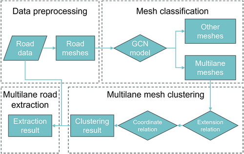
• Data preprocessing: According to the closure principle, road mesh polygons are constructed from the original road network data, and the shape descriptors of the meshes are calculated.

• Mesh classification: According to the topological relationship between road meshes, a graph structure of road meshes is constructed. The meshes are classified into multilane road meshes and other meshes using a semi-supervised classification approach with a GCNN model.

• Mesh clustering and multilane road extraction: Two kinds of spatial relationships, extension relationship and parallel relationship, between adjacent meshes belonging to the same multilane road are extracted. The detected multilane road meshes are clustered into groups considering their spatial relationships, and the clustered road meshes are combined and overlapped with the road network to extract multilane roads at the object level.

3.2. Data preprocessing

Road meshes are constructed considering the closure principle at first. Based on their location, meshes are classified as either multilane road meshes (those located inside multilane roads) or other meshes. Typically, a polygon’s shape is characterized using basic indicators such as area, convexity, compactness, ellipticity and rectangularity. These indicators have been proven effective for classifying polygon shapes (Yan et al. 2019). Considering the unique morphological characteristics of multilane road meshes, various indicators have been proposed in previous studies, which are listed in Table 1, and their meanings are described in Figure 3.

Figure 3. Indicators of individual meshes: (a) demonstrates the relevant parameters of parallelism and elongation, where $L_{\mathit{\text{SBR}}}$ and $W_{\mathit{\text{SBR}}}$ represent the length and width of the minimum bounding rectangle, SBRO indicates the main direction of the minimum bounding rectangle, and Primary Edges are depicted as bold line segments; (b) presents the convex hull and minimum enclosing circle (MEC) of the mesh.

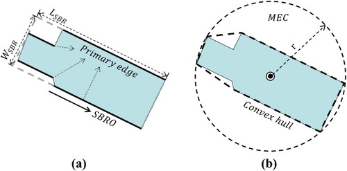
Table 1. Descriptions of the descriptors of individual road meshes.

Index	Notation/equation	Description
Area	$A_m$	Mesh area
Perimeter	$P_m$	Mesh perimeter
Compactness	$\frac{4\pi A_m}{{P_m}^2}$	Quadratic relationship between the area and the perimeter (Touya 2010); The value ranges from 0 to 1, where a circle shape has the highest value of 1
Parallelism	$\sum \frac{L_{\mathit{\text{primary}}\_\mathit{\text{edge}}}}{P_m}$	The ratio of the total length of the primary edges to the mesh perimeter (Li et al. 2014)
Width	$\frac{A_m}{L_{\mathit{\text{centerline}}}}$	The ratio of the mesh area to the length of the centerline (Li et al. 2014)
Concavity	$\frac{A_m}{A_{\mathit{\text{convex}}}}$	Area ratio of a mesh to its convex hull (Basaraner and Cetinkaya 2017)
Circularity	$\frac{A_m}{{\pi r}^2}$	Area ratio of a mesh to its minimum enclosing circle (Xu et al. 2019)
Elongation	$\frac{L_{\mathit{\text{SBR}}}}{W_{\mathit{\text{SBR}}}}$	Length-width ratio of the mesh SBR (Burghardt and Steiniger 2005)

Feature selection plays a crucial role in classification tasks (Peng et al. 2005), which influences the performance and efficiency of the classification model. To ensure that the selected indicators encompass all potential factors influencing the classification results, while minimizing feature correlations, selecting the optimal combination of features is important. Based on the findings of Wu’s (2022) research, this study selects width, perimeter, area, elongation, and compactness as indicators for classification. Among them, width, perimeter and area exhibit a long-tailed distribution. To mitigate outlier influence, they are normalized using Equation (1)(1) $${\left(A_j\right)}_{i\_\mathit{\text{dx}}}=\left|{\mathrm{\text{log}}}_{{A_j}_{\mathrm{\text{max}}}}\left({\left(A_j\right)}_i\right)\right|$$(1) : (1) $${\left(A_j\right)}_{i\_\mathit{\text{dx}}}=\left|{\mathrm{\text{log}}}_{{A_j}_{\mathrm{\text{max}}}}\left({\left(A_j\right)}_i\right)\right|$$(1) where ${(A_j)}_i$ and ${(A_j)}_{i\_\mathit{\text{dx}}}$ are the $j_{\mathit{\text{th}}}$ features of mesh $i$ before and after normalization, respectively, and ${A_j}_{\mathrm{\text{max}}}$ denotes the maximum value of the $j_{\mathit{\text{th}}}$ feature among all meshes.

3.3. Road mesh classification

Different from the existing methods that involve classification only considering the features of individual meshes, this study introduced a GCN-based method to represent and learn mesh features by aggregating the feature information of adjacent meshes in a specific neighborhood to the current mesh.

A graph structure representation $G=(V,E,A)$ of the road meshes is first constructed, where $V$ is the graph node set abstracted from road meshes, $E$ denotes the set of edges between graph nodes. Two meshes are considered adjacent if the geometric intersection between the two meshes forms a line segment. In the graph structure, corresponding graph nodes are connected by edges. $A$ is an adjacency matrix, recording the adjacent relationship between the nodes of the entire graph. $A_{i,j}=1$ if graph node $v_i$ is adjacent to $v_j$ and 0 otherwise.

3.3.1. Graph convolution operation

This study introduces a graph convolution operation based on the graph Fourier transform (Kipf and Welling 2017), which has been effectively used in various vector data analysis tasks, such as building pattern recognition (Yan et al. 2019) and specific structure detection in road networks (Wang et al. 2020; Yang et al. 2022). The Fourier transform is a mathematical technique that transforms a signal between the spatial and frequency domains and expands the signal in the Laplacian eigenfunctions. The Laplace matrix L of a graph is a real symmetric matrix. The graph Fourier transform and the inverse transform of any signal $f(n)$ defined at the vertices of the graph G can be expressed as (2) $$\widehat{f}\left({\lambda }_l\right)=X^{T}f$$(2) (3) $$f\left(n\right)=\mathit{\text{Xf}}$$(3) where $X$ and $X^T$ are a set of orthogonal eigenvectors of the graph Laplacian matrix L, and ${\left\{{\lambda }_l\right\}}_{l=0}^{N-1}$ are their corresponding eigenvalues.

According to the convolution theorem, the convolution of a function $f$ on the graph and a filter $g_{\theta }$ can be expressed as: (4) $$g_{\theta }\mathrm{\hspace{0.17em}*\hspace{0.17em}}f=X{g}_{\theta }\left(\mathrm{\Lambda }\right)X^{T}f$$(4) where $g_{\theta }(\mathrm{\Lambda })$ is a function of the eigenvalues of L. To address the problem of excessively high computational complexity for large-scale graphs in convolution operations, Hammond (2011) proposed a local filter based on Chebyshev polynomials and used it to approximate $g_{\theta }(\mathrm{\Lambda })$ as follows: (5) $$g_{{\theta }^{\prime }}\left(\mathrm{\Lambda }\right)=\sum _{k=0}^{K-1}{\theta }_k^{\prime }{T}_k\left(\tilde{\mathrm{\Lambda }}\right)$$(5) where $T_k\left(x\right)=2x{T}_{k-1}\left(x\right)-T_{k-2}\left(x\right),$ with $T_0\left(x\right)=1,$ $T_1\left(x\right)=x.$ ${\theta }_k^{\prime }$ is the polynomial coefficient vector, and $\tilde{\mathrm{\Lambda }}$ is the scaled eigenvector matrix. The graph convolution operation of the K-order local neighborhood is realized by the K-order Chebyshev polynomials of the Laplace matrix.

3.3.2. GCNN model architecture

The GCNN models can be formed by stacking multiple graph convolutional layers. We adopt a multilayer GCNN model that is oriented toward the classification of graph nodes. As demonstrated in Figure 4, the sample model contains two graph convolutional layers and a fully connected layer.

Figure 4. Architecture of the GCNN model.

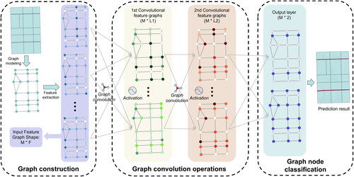
After constructing the graph structure of road meshes, the mesh shape features are extracted as the input node features according to the method in Section 2.2 and then propagated through multiple hidden layers, where the $j_{\mathit{\text{th}}}$ output feature of the ${(l+1)}_{\mathit{\text{th}}}$ hidden layer is calculated as follows: (6) $$H_j^{\left[l+1\right]}=\sigma \left(\sum _{i=1}^N\left(g_{{\theta }^{\prime }}\left(\mathrm{\Lambda }\right)H_i^{\left[l\right]}\right)+b_j^{\left[l\right]}\right)$$(6) where $\sigma (·)$ is a nonlinear activation function, $H_i^{\left[l\right]}$ is the $i_{\mathit{\text{th}}}$ input feature map of the $l_{\mathit{\text{th}}}$ layer, $N$ is the feature dimension of the $l_{\mathit{\text{th}}}$ layer, $g_{{\theta }^{\prime }}\left(\mathrm{\Lambda }\right)$ is a Chebyshev polynomial of order K, and $b_j^{\left[l\right]}$ is the bias of the $l_{\mathit{\text{th}}}$ layer.

The GCNN model is trained by a semi-supervised strategy. A graph with both labeled and unlabeled graph nodes is input into the model. The model propagates information across the graph structure, leveraging both labeled and unlabeled nodes. Initially, the model is trained on the labeled data. The differences between the predicted outcomes and labels (ie, the loss function) are calculated using cross-entropy. The selection of loss function is based on Kipf and Welling (2017), Yan et al. (2019, 2022). By incorporating information from both labeled and unlabeled nodes, the model can effectively utilize the available data to enhance learning outcomes.

The model outputs an $M\times 2$ matrix, with each row containing the classification prediction probability to the corresponding road mesh. The final classification result for each mesh, is determined by the column with the highest probability value in the corresponding row. As illustrated in the prediction results in Figure 4, the red meshes correspond to multilane road meshes, and the blue meshes correspond to other road meshes.

3.4. Meshes clustering and multilane roads extraction

Although the extraction results of multilane road mesh reflect the locations of multilane roads in the road network, they do not indicate the correspondence between road segments and different roads. This information is crucial for various subsequent tasks, including multilane road generalization, road network data matching and updating. To achieve the object-level multilane road extraction, it is necessary to cluster the multilane road meshes into groups based on the corresponding roads to which they belong.

In this study, a bidirectional region growing clustering (BRGC) method for multilane road meshes is proposed based on the extension characteristics between meshes in adjacent lanes and the parallel characteristics between meshes in different lanes of the same multilane road. After clustering, the meshes in each group are separately combined. The extraction results for multilane road are obtained by considering the overlap relationships between the combined meshes and the road network. The BRGC method comprises two progressive steps: (1) detection of the extension relation between meshes and (2) detection of the parallel relation between the combined meshes.

3.4.1. Detection of the extension relation

Approximate distance is often maintained between adjacent lanes of multilane roads. At large scales, the meshes within adjacent lanes are usually characterized by an arrangement extending along the main orientation of the road, such as ${\mathit{\text{mesh}}}_{i-1},{\mathit{\text{mesh}}}_i,\text{and}{\mathit{\text{mesh}}}_{i+1}$ in Figure 5(a). In this article, this arrangement characteristic is defined as the extension relationship. The meshes with an extension relationship are recorded as an extension relationship group. In most straight sections of multilane roads (Figure 5(a)), adjacent road meshes satisfy the following basic construction conditions:

Figure 5. Extension relationship between meshes: (a) straight portion of the multilane roads: $\alpha$ represents the turning angle of the road network contour, $e$ and $\beta$ denotes the common edge and centroid angle between adjacent road meshes, respectively; (b) intersection portion of the multilane roads: ${\mathit{\text{Orient}}}_i$ and ${\mathit{\text{Orient}}}_{i-1}$ represents the main directions of the road meshes; (c) and (d) the extension relationship groups containing long and narrow road meshes ${\mathit{\text{mesh}}}_{\mathit{\text{mid}}}$ and ${\mathit{\text{mesh}}}_{\mathit{\text{end}}}:$ the red rectangle in (d) represents the matching template created by the central road mesh.

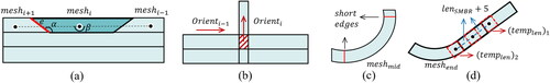
1. Interaction of short edges. The lengths of the common edges of adjacent meshes are less than a certain length. As shown in Figure 5(a), the red line segment e connecting different lanes of the multilane road forms a certain angle $\alpha$ with the lane line features, and its length is relative short to the other edges of the mesh polygon.

2. Straight line arrangement. Adjacent meshes are extended along a specific orientation. As shown in Figure 5(a), this property manifests as the fact that the angle $\beta$ between the centroids of any three adjacent meshes is greater than a certain angle.

3. Consistent principal orientation. The angle $\gamma$ between the principal orientations of adjacent meshes is less than a certain angle. The orientation of the long side of the minimum bounding rectangle of the mesh is used as the principal orientation (Wang and Burghardt 2020).

   Apart from the majority of straight sections, there are also special circumstances that require special handling in specific locations within the road network:

4. Multilane road intersections: The ‘small mesh’ that forms at the intersection of two multilane roads (the mesh represented by the red hatched lines in Figure 5(b)) should belong to two extension relation groups simultaneously. In this case, if Condition C is considered, the extension relation group perpendicular to the principal orientation will be disrupted, resulting in incomplete clustering. Therefore, for a mesh with an area less than the minimum area threshold ${\delta }_{\mathit{\text{minA}}}$ and a number of adjacent meshes not less than 4, condition C is not considered in the detection process.

5. The long curved multilane road meshes (eg, ${\mathit{\text{mesh}}}_{\mathit{\text{mid}}}$ in Figure 5(c) and ${\mathit{\text{mesh}}}_{\mathit{\text{end}}}$ in Figure 5(d)). Compared with that of other meshes, the position of the centroid of these meshes is not fixed, and the angle between the centroids of three adjacent meshes in the same extension relation group may be too large, that is, condition B is not satisfied. In this regard, according to the positions of the curved meshes associated with three adjacent meshes, the following measures are taken:

•   a) If the curved mesh is in the middle position (eg, ${\mathit{\text{mesh}}}_{\mathit{\text{mid}}}$ in Figure 5(c)), only condition A is considered when detecting the extension relation;

•   b) If the curved mesh is located near an edge (eg, ${\mathit{\text{mesh}}}_{\mathit{\text{end}}}$ in Figure 5(d)), a template matching method motivated by Xing et al. (2021) is used to check the extension relation between meshes. With the centroid of ${\mathit{\text{mesh}}}_{\mathit{\text{mid}}}$ as the reference, an initial square template with a side length of 10 m is created, and its orientation is determined by the long side of the SMBR of ${\mathit{\text{mesh}}}_{\mathit{\text{mid}}}.$ The length and width of the SMBR of ${\mathit{\text{mesh}}}_{\mathit{\text{mid}}}$ are defined as ${\mathit{\text{len}}}_{\mathit{\text{SMBR}}}$ and ${\mathit{\text{wid}}}_{\mathit{\text{SMBR}}},$ respectively. The clockwise rotation angles with respect to the true north direction are defined as the edge orientations, denoted as ${\mathit{\text{orient}}}_{\mathit{\text{len}}}$ and ${\mathit{\text{orient}}}_{\mathit{\text{wid}}},$ respectively. The matching templates ${({\mathit{\text{temp}}}_{\mathit{\text{len}}})}_1$ and ${({\mathit{\text{temp}}}_{\mathit{\text{wid}}})}_1$ are created along the above two orientations according to the length of ${\mathit{\text{len}}}_{\mathit{\text{SMBR}}}+5$ and ${\mathit{\text{wid}}}_{\mathit{\text{SMBR}}}+5.$ The area ratios of the intersection of the matching template and the meshes to the area of the corresponding matching template, ${\mathit{\text{IoU}}}_{\mathit{\text{len}}/\mathit{\text{wid}}}=\frac{{\mathit{\text{area}}({\mathit{\text{temp}}}_{\mathit{\text{len}}/\mathit{\text{wid}}}\cap \mathit{\text{mesh}}}_{\mathit{\text{end}}})}{\mathit{\text{area}}({\mathit{\text{temp}}}_{\mathit{\text{len}}/\mathit{\text{wid}}})}$ are calculated. If ${\mathit{\text{IoU}}}_{\mathit{\text{len}}}>0.6$ or ${\mathit{\text{IoU}}}_{\mathit{\text{wid}}}>0.6,$ then a matching template ${({\mathit{\text{temp}}}_{\mathit{\text{len}}})}_2$ or ${({\mathit{\text{temp}}}_{\mathit{\text{wid}}})}_2$ with the same length is constructed with the opposite orientation of the corresponding orientation ${{\mathit{\text{oppo}}}_{\mathit{\text{len}}}=\mathit{\text{orient}}}_{\mathit{\text{len}}}+180$ or ${{\mathit{\text{oppo}}}_{\mathit{\text{wid}}}=\mathit{\text{orient}}}_{\mathit{\text{wid}}}+180.$ If the IoU value between this template and the mesh at the other end is greater than 0.6, then the three meshes are recorded as an extension relation group.

In summary, the framework for detecting extension relationships between multilane meshes (Algorithm A) is illustrated by the flowchart in Figure 6.

Figure 6. The flowchart of Algorithm A.

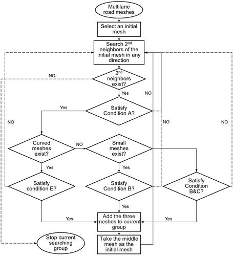
The detailed strategy is as follows (Algorithm A):

• Step 1. Determine the turning point of the mesh polygon boundary based on a rotation angle threshold ${\delta }_{\mathit{\text{TA}}},$ representing the mesh boundary as a set of connected segments.

• Step 2. Select an initial ${\mathit{\text{node}}}_i$ from the graph structure for the current extension relation group.

• Step 3. Search a neighbor ${\mathit{\text{node}}}_j$ of ${\mathit{\text{node}}}_i$ and a neighbor ${\mathit{\text{node}}}_k$ of ${\mathit{\text{node}}}_j$ that both satisfy Condition A.

• Step 4. Check if there are curved meshes among the three meshes. If so, use Condition E to determine if the three meshes have an extension relationship.

• Step 5. If no curved mesh is found, check if there are meshes with an area smaller than the threshold ${\delta }_{\mathit{\text{minA}}}.$ If so, use Condition B to determine if the three meshes have an extension relation.

• Step 6. If neither a curved mesh nor a small mesh is found, Conditions B and C are used to determine the extension relation between the three meshes.

• Step 7. Add the three meshes that satisfy the extension relation to the current extension relation group ${\mathit{\text{Extension}}\_\mathit{\text{list}}}_l$ in order.

• Step 8. Continue searching for neighbor nodes starting from ${\mathit{\text{node}}}_j$ and ${\mathit{\text{node}}}_k.$

• Step 9. Repeat steps 3–8 until no new mesh with the extension relation can be detected at both ends of the current extension relation group.

• Step 10.  Select a new start node from the graph structure and repeat the above steps until all nodes have been processed.

• Step 11.  Merge the meshes in the same extension relation group and store them into the combined extension mesh list $\mathit{\text{eMesh}}\_\mathit{\text{list}}.$

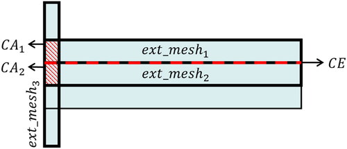
3.4.2. Parallel relation detection and multilane road extraction

The combined meshes obtained by Algorithm A usually exhibit elongated characteristics, as ${\mathit{\text{ext}}\_\mathit{\text{mesh}}}_1,$ ${\mathit{\text{ext}}\_\mathit{\text{mesh}}}_2$ and ${\mathit{\text{ext}}\_\mathit{\text{mesh}}}_3$ shown in Figure 7. We define the relationship between adjacent meshes belonging to the same road as parallel relation (the relationship between ${\mathit{\text{ext}}\_\mathit{\text{mesh}}}_1$ and ${\mathit{\text{ext}}\_\mathit{\text{mesh}}}_2$). The intersection of the two meshes is a line segment $\mathit{\text{CE}}$ (red dashed line) that overlaps one of the lanes of the multilane road. ${\mathit{\text{Ext}}\_\mathit{\text{mesh}}}_1$ and ${\mathit{\text{ext}}\_\mathit{\text{mesh}}}_3,$ as well as ${\mathit{\text{ext}}\_\mathit{\text{mesh}}}_2$ and ${\mathit{\text{ext}}\_\mathit{\text{mesh}}}_3$ are meshes associated with different roads, with no parallel relation. Their intersections are polygons ${\mathit{\text{CA}}}_1$ and ${\mathit{\text{CA}}}_2.$

Figure 7. The parallel relationship between meshes: $\mathit{\text{CE}}$ represents the common segment of ${\mathit{\text{ext}}\_\mathit{\text{mesh}}}_1$ and ${\mathit{\text{ext}}\_\mathit{\text{mesh}}}_2;$ ${\mathit{\text{CA}}}_1$ and ${\mathit{\text{CA}}}_2$ denote the common areas of ${\mathit{\text{ext}}\_\mathit{\text{mesh}}}_1$ and ${\mathit{\text{ext}}\_\mathit{\text{mesh}}}_3$ and ${\mathit{\text{ext}}\_\mathit{\text{mesh}}}_2$ and ${\mathit{\text{ext}}\_\mathit{\text{mesh}}}_3,$ respectively.

Building upon the common geometric types of road meshes after processing with Algorithm A, this article proposes an approach (Algorithm B) to detect parallel relationship and extract the multilane roads. The specific steps are as follows:

• Step 1. Randomly select ${\mathit{\text{ext}}\_\mathit{\text{mesh}}}_i\mathrm{ }$ from the $\mathit{\text{eMesh}}\_\mathit{\text{list}}.$ Find another mesh ${\mathit{\text{ext}}\_\mathit{\text{mesh}}}_j$ that is topologically adjacent to ${\mathit{\text{ext}}\_\mathit{\text{mesh}}}_i.$ Calculate the length $L_{i,j}$ of the common edge between the two meshes.

• Step 2. If $L_{i,j}>{\delta }_{\mathit{\text{LC}}},$ store ${\mathit{\text{ext}}\_\mathit{\text{mesh}}}_j$ in the ${\mathit{\text{Coordinate}}\_\mathit{\text{list}}}_l.$

• Step 3. Repeat steps 2 and 3 until no new meshes with a parallel relation are found to the current meshes.

• Step 4. Remove the meshes in ${\mathit{\text{Coordinate}}\_\mathit{\text{list}}}_l$ from $\mathit{\text{eMesh}}\_\mathit{\text{list}}$ and merge them. Store the combined mesh into the combined parallel mesh list $\mathit{\text{cMesh}}\_\mathit{\text{list}}.$

• Step 5. Repeat steps 1 to 4 until $\mathit{\text{eMesh}}\_\mathit{\text{list}}$ is empty.

• Step 6. Based on the overlap relationship between road segments and the meshes in $\mathit{\text{cMesh}}\_\mathit{\text{list}},$ extract multilane roads at the object level.

4. Experiments and analysis

To validate the effectiveness of the proposed approach, we conducted experiments on the real-world data from the OpenStreetMap website. This section presents a description of the experimental data and process, as well as an analysis and discussion of the obtained results.

4.1. Experimental data and preprocessing

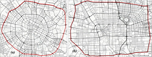
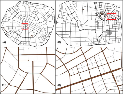
Two cities with highly developed road transportation systems, Chengdu, and Zhengzhou, were selected as the experimental areas. Dataset 1 is comprised of the Chengdu Ring Expressway and its inner roads, while dataset 2 includes the Third Ring Road of Zhengzhou and its internal roads. Figure 8 displays the road network data for the experimental areas in the two cities (road networks within the red rings).

Figure 8. Experimental data of the two cities.

Road meshes were constructed and classified according to section 2.2 are shown in Table 2. To assess the completeness of the multilane roads extraction result, the multilane road segments in the two datasets were manually labeled. Additionally, considering features such as road names and extensibility, the multilane road segments were grouped according to the roads to which they belong. The statistics for each type of road mesh, the total length and the number of multilane roads groups for both datasets are shown in Table 2.

Table 2. Sample set statistics.

	Multilane road mesh	Other mesh	Total mesh	Total length of multilane road (km)	Number of multilane roads
Chengdu	3986	1426	5412	1412.82	151
Zhengzhou	4063	1799	5862	1520.16	139

4.2 Experimental results and analysis

4.2.1. Classification results of multilane road meshes

The semi-supervised learning strategy described in section 3.3.2 was employed to initially train the GCNN model. Following the construction of the road meshes in the form of graph structures, the graph nodes were divided into training and testing sets, adhering to a predefined ratio. In this section, we conducted experiments to test the sensitivity of the GCNN model to parameters and compared the classification accuracy of different methods.

(1) Parameter sensitive analysis

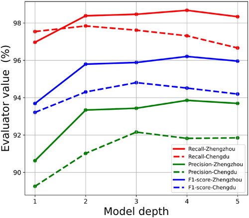
Based on the approach outlined in section 3.2, four descriptors of road mesh were first computed, and the graph representations of the two datasets were established. We conducted two sets of experiments to investigate several factors that influence the classification performance of the proposed model, including model depth, Chebyshev polynomials order, and input variables. Three classic evaluators, ie, recall, precision and f1-score, are selected to evaluate the classification results of multilane road meshes, which are calculated as follows: (7) $$\mathit{\text{Recall}}=\frac{\mathit{\text{TP}}}{\mathit{\text{TP}}+\mathit{\text{FN}}}\times 100\mathrm{\%}$$(7) (8) $$\mathit{\text{Preci}}\mathrm{s}\mathit{\text{ion}}=\frac{\mathit{\text{TP}}}{\mathit{\text{TP}}+\mathit{\text{FP}}}\times 100\mathrm{\%}$$(8) (9) $$\mathit{\text{IoU}}=\frac{\mathit{\text{TP}}}{\mathit{\text{TP}}+\mathit{\text{FP}}+\mathit{\text{FN}}}\times 100\mathrm{\%}$$(9)

Since the proposed GCNN model contains only several convolutional layers and a fully connected layer, the model depth can be varied by adjusting the number of convolutional layers. The model depth varied from 1 to 5 layers. To ensure a controlled environment, we used four features as the model’s input feature and labeled 35% of the graph nodes. The training and testing sets were balanced in terms of the distribution between multilane road meshes and other types of meshes. Each convolutional layer was approximated by first-order Chebyshev polynomials. Figure 9 reports the results on two datasets with different model depths. The results show that as the model depth increased from 1 to 3, there was a consistent improvement in precision, recall, and f1-score. However, as the model depth continued to increase, a declining trend emerged. One possible reason for this trend could be that as the model depth increases beyond a certain point, it becomes more prone to overfitting. The model starts to memorize the training data instead of learning general patterns, resulting in decreased performance on unseen data. Additionally, deeper models may become more complex and harder to optimize, leading to diminishing returns or even degradation in performance.

Figure 9. Model performances varying the model depth.

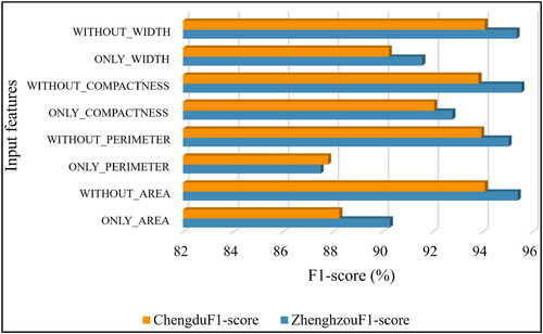
Figure 10 shows the performances by using only one descriptive indicator at a time or all the indicators except for one as the input features. The model adopted a four-layer-depth architecture with other hyperparameter remained the same with the previous experiment. The f1-score of the model’s classification results slightly decreases when one of the input factors missing. It indicates that the model relies on each of the four indicators to make accurate predictions. For individual indicator, relatively higher f1-scores were achieved when only the compactness or width indicator was considered, suggesting that these two indicators played a more crucial role when extracting multilane road meshes. This might be attributed to the narrow and long characteristics of the multilane road meshes, with the values of width and compactness aptly emphasizing the slender attributes of the polygons.

Figure 10. Model performances varying different indicators as input features.

(2) Comparative analysis

A three-layer GCNN model was applied as the model architecture. A classic machine learning method, support vector machine (SVM), which has been introduced to multilane road mesh classification, was chosen for comparative trial. We utilized a semi-supervised learning approach to train both the GCNN model and SVM method, where 15%, 25%, and 35% of the graph nodes were randomly selected for the training set. The remaining nodes were utilized as the testing set to evaluate the model’s performance. F1-score was used as the metric to evaluate the classification performance, as it considered both precision and recall, providing a balanced assessment of a model’s performance. Figure 11 illustrates the f1-score value of all methods across the two datasets under different label rates.

Figure 11. The f1-score of multilane road mesh detection results by the SVM and GCN models on two datasets.

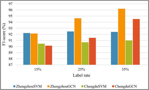
The comparison of the experimental results revealed that both approaches achieved high accuracy with a small number of samples. Specifically, on the Zhengzhou dataset, the f1-scores of both models surpassed 92%, whereas on the Chengdu dataset, the f1-scores of the two models exceeded 90%. A detailed analysis of the results of the two models is given below:

First, the SVM model slightly outperforms the GCNN model with a label rate of 15%. At 25% and 35% label rate, the GCNN model demonstrates significantly superior performance compare to the SVM model. The possible reasons that the GCNN model outperforms the SVM models are as follows: first, since GCNN is specifically designed to handle data with graph structure, it can effectively capture the relationships and dependencies between nodes in the graph, which may contain important information for classification tasks. Moreover, GCNN can learn feature representations directly from graph-structured data through message passing between neighboring nodes in the graph. This allows the model to automatically extract relevant features and patterns, potentially leading to better representations for classification.

Second, there is a consistent increase in accuracy for the GCNN model in both datasets while the label rate increases. This suggests that the GCNN model requires a greater number of training samples to ensure optimal performance compared to the SVM model, possibly due to the larger number of trainable parameters in the model. In addition, the ability to utilize graph structure may account for this trend. GCN is specifically designed to leverage the structural information encoded in graph data. As the label rate increases, providing more labeled data, GCN can effectively exploit the relationships between nodes in the graph to improve its performance.

The results of the multilane road mesh extraction on two datasets were imported into ArcMap and shown in Figure 12(a) and (b), respectively. Figure 12(c) and (d) give detailed presentations of the local region.

Figure 12. Multilane road mesh extraction results. Global for (A) Chengdu and (B) Zhengzhou, (C) and (D) are local for them.

3.2.2. Mesh clustering and multilane road extraction results

Based on the classification results of multilane road meshes, the BRGC method in Section 2.4 was implemented to divide the multilane road meshes into different groups according to the road to which they belong. Some obviously erroneous extracted multilane meshes are removed before the algorithm implementation. Considering the characteristics and parameter tuning experiments, the parameter thresholds involved in the method are set as follows (Table 3).

Table 3. Parameter setting for Algorithm A and B.

Algorithm	Parameter	Value
A	${\delta }_{\mathit{\text{TA}}}$	$17°$
A	${\delta }_{\mathit{\text{EL}}}$	$180 m$
A	${\delta }_{\mathit{\text{minA}}}$	$500{ m}^2$
B	${\delta }_{\mathit{\text{CL}}}$	$100 m$

Figures 13 and 14 depict the implementation process of the BRGC algorithm for extracting object-level multilane roads on datasets from Chengdu and Zhengzhou, respectively. To illustrate the results clearly, we selected typical regions in each dataset for detailed presentation. Subfigure (A) shows the multilane road meshes detected by the GCNN model. Multilane road meshes with extension relationships were first clustered and merged using algorithm A. The generated combined meshes are distinguished by different colors in subfigures (B). The road meshes in subfigures (C), depicted in varying colors, represent the combined road meshes with parallel relationships obtained using algorithm B. Subfigures (E) displays the extraction result of multilane roads, with road segments associated with different roads shown in distinct colors, while the gray roads denote single-lane roads.

Figure 13. The implementation process of BGRC in Chengdu dataset. The multilane road meshes (subfigure (a)) are first clustered and merged using algorithm A (subfigure (B)), and then processed by algorithm B (subfigure (C)). the object-level extraction results of multilane roads are represented in subfigure (C) by various colors.

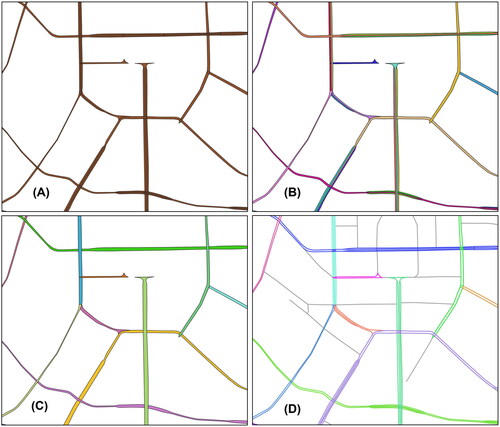
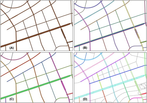
Figure 14. The implementation process of BGRC in Zhengzhou dataset. The multilane road meshes (subfigure (a)) are first clustered and merged using algorithm A (subfigure (B)), and then processed by algorithm B (subfigure (C)). the object-level extraction results of multilane roads are represented in subfigure (C) by various colors.

The experimental results unequivocally showcase the efficacy of algorithm A in accurately discerning the extension relationship between adjacent road meshes, thereby adeptly clustering them within the same lane. Leveraging this outcome, algorithm B efficiently clusters and amalgamates the road meshes based on their parallel relationships. Finally, the road segments associated with different roads are accurately extracted, realizing the object-level extraction of multilane roads.

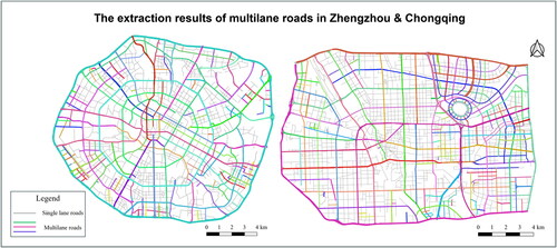
The extraction results of multilane road on the two datasets are displayed in Figure 15. Bold road segments, distinguished by various colors, denote distinct multilane road sections belonging to separate roads, whereas gray segments signify single-lane roads that remained unextracted.

Figure 15. Extraction results for multilane roads in two datasets, where the bold road segments in various colors denote the extracted multilane roads associated with different roads, whereas the grey segments denote the single-lane road.

3.2.3. Evaluation and analysis of the extraction results

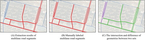
To measure the completeness of the multilane road extraction results, the experimental results were quantitatively evaluated by comparing the intersection and difference of geometries between the extracted and manually labeled multilane roads. The sets of extracted and labeled multilane road segments were denoted as $S_A$ and $S_B,$ as illustrated by the red road segments in Figure 16(A) and (B), respectively. The intersection of the two sets $S_A\cap S_B$ (represented by the green road segments in Figure 16(C)) comprised the correctly extracted multilane road segments (true-positive/TP), and their length was denoted as true-positive (TP). The complement of $S_B$ in $S_A$ (illustrated by the red road segments in Figure 16(C)) represented the multilane road segments that have been mistakenly extracted, and their length was denoted as false-positive (FP). The complement of $S_A$ in $S_B$ (represented by the purple road segments in Figure 16(C)) contained the misidentified multilane road segments, and their length was denoted as false-negative (FN).

Figure 16. The intersection and difference of geometries between the extracted and labeled multilane road.

The conventional evaluation metrics in the machine learning, namely precision, recall, and intersection over union (IoU), were used to evaluate the effectiveness of the proposed approach, as calculated using Equations (7)–(9). The statistical results for the two datasets are shown in Table 4.

Table 4. Statistics and evaluation of the multilane road extraction results.

	TP (km)	FP (km)	FN (km)	Precision (%)	Recall (%)	IoU (%)
Chengdu	1393.94	48.66	18.89	96.63	98.66	95.38
Zhengzhou	1500.92	64.09	19.24	95.90	98.73	94.74

As shown in Table 4, the recall rates for both datasets exceeded 98.5%, indicating that the majority of the multilane roads in the two road networks were accurately extracted. The precision values for the two datasets were 96.63% and 95.90%, respectively, suggesting that a small number of multilane roads were erroneously extracted. An in-depth analysis revealed that extraction errors mainly occurred at complex intersections, such as interchanges, where certain ramps connecting main roads were misidentified as multilane roads.

Furthermore, to assess the effectiveness of the proposed BRGC method, the extraction results were quantitatively evaluated at the object level. As illustrated in Figure 17(A) and (B), the extracted and labeled multilane roads of the cities were stored in two lists, ${\mathit{\text{List}}}_{\mathit{\text{detected}}}$ and ${\mathit{\text{List}}}_{\mathit{\text{labeled}}},$ respectively. Each multilane road was treated as an individual object. A verification process was conducted to evaluate the precision of the extraction of each multilane road, utilizing the IoU value (${\mathit{\text{IoU}}}_M$) as a metric to compare the detected instances of road with their corresponding labeled roads. Assuming $M_A$ denote a specific detected multilane road, while $M_B$ denote a labeled multilane road, the ${\mathit{\text{IoU}}}_M$ value between these two roads is defined as follows: (10) $${\mathit{\text{IoU}}}_M=\frac{\mathit{\text{Len}}(M_A\hspace{0.17em}\bigcap \hspace{0.17em}{M}_B)}{\mathit{\text{Len}}(M_A\hspace{0.17em}\bigcup \hspace{0.17em}{M}_B)}$$(10) where $\mathit{\text{Len}}(M_A\bigcap M_B)$ and $\mathit{\text{Len}}(M_A\bigcup M_B)$ denote the total lengths of the intersection and union between $M_A$ and $M_B.$ With regard to the IoU threshold for object detection tasks, this study selected 0.8 as the threshold for assessing the accurate extraction of multilane roads. A value of ${\mathit{\text{IoU}}}_M\ge 0.8$ signified a correctly extracted multilane road, labeled as TP–MR (depicted by the roads in Figure 17(C)), while ${\mathit{\text{IoU}}}_M<0.8$ indicated the absence of a matching relationship between the two multilane roads. Road features in ${\mathit{\text{List}}}_{\mathit{\text{detected}}}$ without corresponding matches in ${\mathit{\text{List}}}_{\mathit{\text{labeled}}}$ were labeled as FP-MR (shown as the roads in Figure 17(D)), while roads in ${\mathit{\text{List}}}_{\mathit{\text{labeled}}}$ without corresponding matches in ${\mathit{\text{List}}}_{\mathit{\text{detected}}}$ were labeled as FN–MR (represented by the roads in Figure 17(E)). Table 5 shows the statistics of the numbers of TP–MR, FP–MR and FN–MR roads in the extraction results. The recall and precision of the object-level road extraction results are calculated using Equations (7)(7) $$\mathit{\text{Recall}}=\frac{\mathit{\text{TP}}}{\mathit{\text{TP}}+\mathit{\text{FN}}}\times 100\mathrm{\%}$$(7) and (8)(8) $$\mathit{\text{Preci}}\mathrm{s}\mathit{\text{ion}}=\frac{\mathit{\text{TP}}}{\mathit{\text{TP}}+\mathit{\text{FP}}}\times 100\mathrm{\%}$$(8) .

Figure 17. Results of multilane road extraction in two cities.

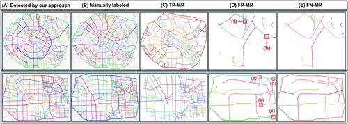
Table 5. Statistics of the multilane road extraction results at the object level.

	TP–MR	FP–MR	FN–MR	Precision–MR (%)	Recall–MR (%)
Chengdu	140	19	11	88.05	92.72
Zhengzhou	127	19	12	86.99	91.37

The result reveals that the proposed method can effectively extract multilane roads at the object level with satisfactory quality, achieving a precision of over 86% and a recall exceeding 90%. Specifically, 140 out of the 151 multilane roads from the Chengdu dataset and 127 out of the 139 multilane roads from the Zhengzhou dataset had an IoU value greater than 0.8, indicating the effectiveness of our method in comprehensively extracting multilane roads from complex road networks. Moreover, the low number of errors in the extraction process, with only 19 roads incorrectly identified in both the two datasets, respectively, further confirms the high reliability of our approach.

Figure 18 provides a detailed demonstration of cases with both erroneous extractions and omitted extractions in the multilane road extraction results, with subfigures showing the corresponding rectangular ranges of the same letters in the FR–MR subfigures of Figure 17. We observed that these errors can be categorized into two cases.

Figure 18. Examples of inaccurate extraction.

The first case involves incomplete extraction due to disruptions in the extension relationships detected during the execution of algorithm A. The main causes of extension relationship disruption are twofold. Firstly, when two road segments with roughly the same direction intersect, they form a small angle (eg, $\mathit{\text{Angle}}\_a$ and $\mathit{\text{Angle}}\_b$ in yellow meshes in Figure 18(a) and (b)) that is smaller than the turning angle threshold ${\delta }_{\mathit{\text{TA}}}$ set in algorithm A. When detecting extension relationships, the meshes formed by these road segments do not satisfy the interaction of short edges rule (condition A in 2.4.1), resulting in the disruption of extension relationships. Secondly, certain ring roads form groups of meshes with extension directions approximately perpendicular to each other at the locations of interchanges, making them difficult to be effectively identified only through geometric methods (eg, the East Third Ring Road and the South Third Ring Road Figure 18(c), and the East Third Ring Road and the North Third Ring Road Figure 18(d) in Zhengzhou City).

The second case arises from specific ramp segments at interchanges forming road meshes linking two multilane roads ($\mathit{\text{Mesh}}\_e$ in Figure 18(e), and $\mathit{\text{Mesh}}\_f$ in Figure 18(f)), where algorithm B erroneously clusters meshes meant for distinct multilane roads, resulting in the erroneous inclusion of more than two roads in the extracted multilane road (eg, the multilane road in Figure 18(e) contains both road $\mathit{\text{MR}}\_e1$ and $\mathit{\text{MR}}\_e2,$ and the multilane road in Figure 18(f) contains both road $\mathit{\text{MR}}\_f1$ and $\mathit{\text{MR}}\_f2$).

3.3. Discussion

3.3.1. Characteristics of the proposed method

The experimental results verify that the proposed method can effectively extract multilane roads in urban road networks. The extraction results are in line with the actual conditions and human cognition. Compared with the existing multilane road identification methods, the proposed method has the following two characteristics:

First, the GCNN model considers the correlations among the local features of road meshes. This represents a significant advancement in deep learning, specifically in the field of convolutional deep learning, where novel vector features are derived through convolution operations. By extracting high-level structural features from shallow geometric features, the GCNN model can better differentiate between multilane road meshes and other types of road meshes.

Second, the extraction of multilane roads at the object level is addressed. The existing multilane road extraction methods based on road meshes can address the extraction of multilane roads at the ‘feature’ level, whereas applications such as map matching and cartographic generalization require the individual processing of specific multilane roads. To address this challenge, clustering based on the spatial relationships among multilane road meshes is performed to achieve the extraction of multilane roads at the object level. Comparatively, the results obtained with the proposed method exhibit greater semantic granularity and hold greater practical value than the current methods.

3.3.2. Limitations

Our method has the following limitations that should be further addressed in future research.

First, due to the irregular features of road meshes in some interchange areas, the multilane roads that visually appear as a single entity are fragmented. The complex and unpredictable shape of road meshes in these areas poses a challenge for clustering and grouping based solely on spatial relationships. To address this issue in future research, we plan to first identify the interchange segments in the road network and subsequently develop algorithms that align with human visual cognition for more accurate multilane road extraction.

Second, due to the reliance on closed polygonal regions formed by road segments, the proposed method based on road meshes fails to identify a small number of suspended multilane roads within the road networks. This limitation represents an inherent defect in all mesh-based methods.

5. Conclusion

Considering the significant differences in geometry among the meshes within multilane roads and other road meshes, this paper proposes a multilane road extraction method based on road meshes. First, a GCNN model is used to comprehensively consider the geometric features of the road meshes themselves and other meshes in the local neighborhood to extract the multilane road meshes. Then, the clustering of multilane road meshes is realized with a region-growing method in both the vertical and horizontal dimensions according to the spatial relationship among the multilane road meshes. Finally, the extraction of multilane roads at the object level is realized based on the spatial relationship between the grouped meshes and the road networks.

The effectiveness of the proposed method is validated using road network data from two cities, Chengdu and Zhengzhou. The experimental results demonstrate that the GCNN model obtained satisfactory results when classifying multilane road mesh, with an f1-score over 90% on both datasets. Moreover, the object-level extraction results of multilane roads achieved a precision and recall of 88.05% and 92.72% for the Chengdu dataset and 86.99% and 91.37% for the Zhengzhou dataset.

Furthermore, there are some limitations of the proposed method. First, the irregular features of road mesh in interchange areas lead to fragmentation of visually connected multilane roads, making clustering and grouping difficult based solely on spatial relationships. Second, some suspended multilane roads that fail to form closed polygonal regions were not extracted, which is an intrinsic deflect of the mesh-based methods. Further research can refer to the detection of complex interchange structures in road network, as they are prevalent and play a crucial role in the connectivity of road networks. Moreover, simplifying and re-representing the detected multilane roads may be a direction for future research, as it is crucial for tasks such as map matching and cartographic generalization.

Acknowledgments

This work was supported by the National Natural Science Foundation of China [42371461].

Disclosure statement

The authors declare that they have no known competing financial interests or personal relationships that could have appeared to influence the work reported in this paper.

Additional information

Funding

This work was supported by the National Natural Science Foundation of China [42371461].

References

- Ali Abbaspour R, Chehreghan A, Karimi A. 2018. Assessing the efficiency of shape-based functions and descriptors in multi-scale matching of linear objects. Geocarto Int. 33:879–892. doi: 10.1080/10106049.2017.1316777.
- Basaraner M, Cetinkaya S. 2017. Performance of shape indices and classification schemes for characterising perceptual shape complexity of building footprints in GIS. Int J Geogr Inf Sci. 31:1952–1977. doi: 10/ghz25g.
- Burghardt D, Steiniger S. 2005. Usage of principle component analysis in the process of automated generalisation. In: Proceeding of the 22th International Cartographic Conference (ICC), p. 9–16.
- Chehreghan A, Ali Abbaspour R. 2018. A geometric-based approach for road matching on multi-scale datasets using a genetic algorithm. Cartograph Geograph Inform Sci. 45(3):255–269. doi: 10.1080/15230406.2017.1324823.
- Chen J, Hu Y, Li Z, Zhao R, Meng L. 2009. Selective omission of road features based on mesh density for automatic map generalization. Int J Geogr Inf Sci. 23:1013–1032. doi: 10.1080/13658810802070730.
- Gong X, Wu F, Xing R, Du J, Liu C. 2021. LCBRG: a lane-level road cluster mining algorithm with bidirectional region growing. Open Geosci. 13:835–850. doi: 10.1515/geo-2020-0271.
- Grigorescu I, Kucsicsa G, Mitrică B, Mocanu I, Dumitrașcu M. 2022. Driving factors of urban sprawl in the Romanian plain. Regional and temporal modelling using logistic regression. Geocarto Int. 37:7220–7246. doi: 10.1080/10106049.2021.1967465.
- Gülgen F. 2014. Road hierarchy with integration of attributes using fuzzy-AHP. Geocarto Int. 29:688–708. doi: 10.1080/10106049.2013.837102.
- Guo X, Liu J, Wu F, Qian H. 2023. A method for intelligent road network selection based on graph neural network. ISPRS International Journal of Geo-Information. 12(8):336. doi: 10.3390/ijgi12080336.
- Guo Q, Xie Y, Liu J, Wang L, Zhou L. 2017. Algorithms for road networks matching considering scale variation and data update. Acta Geo Cartograph Sinica. 46(3):381–388. doi: 10.11947/j.AGCS.2017.20160364.
- Heinzle F, Anders K-H, Sester M. 2006. Pattern recognition in road networks on the example of circular road detection. In Raubal M, Miller HJ, Frank AU, Goodchild MF, editors. Geographic information science, lecture notes in computer science. Berlin, Heidelberg: Springer Berlin Heidelberg, p. 153–167. doi: 10.1007/11863939_11.
- Hong Y, Yao Y. 2019. Hierarchical community detection and functional area identification with OSM roads and complex graph theory. Int J Geogr Inf Sci. 33:1569–1587. doi: 10.1080/13658816.2019.1584806.
- Hu Z, Jia T, Wang G, Wang J, Meng L. 2017. Computing a hierarchy favored optimal route in a Voronoi-based road network with multiple levels of detail. Int J Geogr Inf Sci. 31:2216–2233. doi: 10.1080/13658816.2017.1356460.
- Jiang B. 2009. Street hierarchies: a minority of streets account for a majority of traffic flow. Int J Geogr Inf Sci. 23:1033–1048. doi: 10.1080/13658810802004648.
- Kim I-H, Feng C-C, Wang Y-C. 2017. A simplified linear feature matching method using decision tree analysis, weighted linear directional mean, and topological relationships. Int J Geograph Inform Sci. 31:1042–1060. doi: 10.1080/13658816.2016.1267736.
- Kipf TN, Welling M. 2017. Semi-supervised classification with graph convolutional networks. In: Proceedings of the 5th International Conference on Learning Representations (ICLR), p. 1–14. doi: 10.48550/arXiv.1609.02907.
- Li Q, Fan H, Luan X, Yang B, Liu L. 2014. Polygon-based approach for extracting multilane roads from OpenStreetMap urban road networks. Int J Geogr Inf Sci. 28:2200–2219. doi: 10.1080/13658816.2014.915401.
- Li Y, Fei T, Zhang F. 2019. A regionalization method for clustering and partitioning based on trajectories from NLP perspective. Int J Geogr Inf Sci. 33:2385–2405. doi: 10.1080/13658816.2019.1643025.
- Liu C, Zhai R, Qian H, Gong X, Wang A, Wu F. 2023. Identification of drainage patterns using a graph convolutional neural network. Trans GIS. 27(3):752–776. doi: 10.1111/tgis.13041.
- Liu K, Gao S, Lu F. 2019. Identifying spatial interaction patterns of vehicle movements on urban road networks by topic modelling. Comput Environ Urban Syst. 74:50–61. doi: 10.1016/j.compenvurbsys.2018.12.001.
- Mann D, Rankavat S, Joshi PK. 2022. Road network drives urban ecosystems - a longitudinal analysis of impact of roads in the central Himalaya. Geocarto Int. 37:1100–1125. doi: 10.1080/10106049.2020.1750064.
- Martin K. 2024. Learning from Vector Data: Enhancing Vector-Based Shape Encoding and Shape Classification for Map Generalization Purposes. Cartography and Geographic Information Science. 51(1):146–167. doi: 10.1080/15230406.2023.2273397.
- Peng H, Long F, Ding C. 2005. Feature selection based on mutual information criteria of max-dependency, max-relevance, and min-redundancy. IEEE Transactions on Pattern Analysis and Machine Intelligence. 27(8):1226–1238. doi: 10.1109/TPAMI.2005.159.
- Shoman W, Gülgen F. 2017. Centrality-based hierarchy for street network generalization in multi-resolution maps. Geocarto Int. 32:1352–1366. doi: 10.1080/10106049.2016.1208683.
- Stefanakis E. 2015. SELF: semantically enriched line simplification. Int J Geogr Inf Sci. 29:1826–1844. doi: 10.1080/13658816.2015.1053092.
- Thom S. 2002. A strategy for collapsing OS Integrated Transport NetworkTM dual carriageways. Presented at the 8th ICA workshop on generalisation and multiple representations, Leicester, UK.
- Tong X, Liang D, Jin Y. 2014. A linear road object matching method for conflation based on optimization and logistic regression. Int J Geogr Inf Sci. 28:824–846. doi: 10.1080/13658816.2013.876501.
- Touya G. 2010. A road network selection process based on data enrichment and structure detection: road network selection. Trans GIS. 14:595–614. doi: 10/d2vj6k.
- Wang M, Ai T, Yan X, Xiao Y. 2020. Grid pattern recognition in road networks based on graph convolution network model. Geomat Inform Sci Wuhan Univ. 45(12):1960–1969. doi: 10.13203/j.whugis20200022.
- Wang D, Qian H. 2023. Graph neural network method for the intelligent selection of river system. Geocarto International. 38(1):2252762. doi: 10.1080/10106049.2023.2252762.
- Wang W, Yan H, Lu X, He Y, Liu T, Li W, Li P, Xu F. 2023. Drainage pattern recognition method considering local basin shape based on graph neural network. Int J Digital Earth. 16(1):593–619. doi: 10.1080/17538947.2023.2172224.
- Wang X, Burghardt D. 2020. Using stroke and mesh to recognize building group patterns. Int J Cartogr. 6:71–98. doi: 10/gnpwzf.
- Wang X, You S, Wang L. 2017. Classifying road network patterns using multinomial logit model. J Transp Geogr. 58:104–112. doi: 10.1016/j.jtrangeo.2016.11.013.
- Wu K, Xie Z, Hu M. 2022. An unsupervised framework for extracting multilane roads from OpenStreetMap. Int J Geogr Inf Sci. 36:2322–2344. doi: 10.1080/13658816.2022.2107208.
- Xing R, Wu F, Gong X, et al. 2021. The template matching approach to combined collinear pattern recognition in building groups. Acta Geodaet Cartograph Sinica, 50(6):800–811. doi: 10.11947/j.AGCS.2021.20200298.
- Xing R, Wu F, Zhang H, Gong X. 2018. Dual-carriageway road extraction based on facing project distance. Geomat Inform Sci Wuhan Univ. 43(1):152–158. doi: 10.13203/j.whugis20150783.
- Xu Y, Xie Z, Wu L, Chen Z. 2019. Multilane roads extracted from the OpenStreetMap urban road network using random forests. Trans GIS. 23:224–240. doi: 10.1111/tgis.12514.
- Yan X, Ai T, Yang M, Tong X, Liu Q. 2020. A graph deep learning approach for urban building grouping. Geocarto Int. 37(10):2944–2966. doi: 10.1080/10106049.2020.1856195.
- Yan X, Ai T, Yang M, Tong X. 2021. Graph convolutional autoencoder model for the shape coding and cognition of buildings in maps. Int J Geogr Inf Sci. 35(3):490–512. doi: 10.1080/13658816.2020.1768260.
- Yan X, Ai T, Yang M, Yin H. 2019. A graph convolutional neural network for classification of building patterns using spatial vector data. ISPRS J Photogramm Remote Sens. 150:259–273. doi: 10.1016/j.isprsjprs.2019.02.010.
- Yang B, Luan X, Li Q. 2011. Generating hierarchical strokes from urban street networks based on spatial pattern recognition. Int J Geogr Inf Sci. 25:2025–2050. doi: 10/bpwt3x.
- Yang M, Jiang C, Yan X, Ai T, Cao M, Chen W. 2022. Detecting interchanges in road networks using a graph convolutional network approach. Int J Geogr Inf Sci. 36:1119–1139. doi: 10.1080/13658816.2021.2024195.
- Yu H, Ai T, Yang M, Huang L, Yuan J. 2022. A recognition method for drainage patterns using a graph convolutional network. Int J Appl Earth Obs Geoinformation. 107:102696. doi: 10.1016/j.jag.2022.102696.
- Yu H, Ai T, Yang M, Huang W, Harrie L. 2023. A graph autoencoder network to measure the geometric similarity of drainage networks in scaling transformation. Int J Digital Earth. 16(1):1828–1852. 10.1080/17538947.2023.2212920.
- Yu W, Zhang Y, Ai T, Guan Q, Chen Z, Li H. 2020. Road network generalization considering traffic flow patterns. Int J Geogr Inf Sci. 34:119–149. doi: 10.1080/13658816.2019.1650936.
- Zhang H, Wu F, Zhang J, Li J. 2016. A method considering shape feature and semantic information for dual-carriageway roads recognition. J Geomat Sci Technol. 33(3):301–305 + 312. doi: 10.3969/j.issn.1673-6338.2016.03.016.
- Zhao R, Ai T, Yu W, He Y, Shen Y. 2020. Recognition of building group patterns using graph convolutional network. Cartograph Geograph Inform Sci. 47(5):400–417. doi: 10.1080/15230406.2020.1757512.
- Zhou Q, Li Z. 2016. Empirical determination of geometric parameters for selective omission in a road network. Int J Geogr Inf Sci. 30:263–299. doi: 10.1080/13658816.2015.1085538.
- Zhou Z, Fu C, Weibel R. 2023. Move and remove: multi-task learning for building simplification in vector maps with a graph convolutional neural network. ISPRS J Photogramm Remote Sens. 202:205–218. doi: 10.1016/j.isprsjprs.2023.06.004.