Warming inland water in peninsular Spain revealed by landsat 5 analysis

Abstract

Lakes and reservoirs provide habitat for a wide range of species and are essential components of numerous ecosystems. In Spain, these water bodies are particularly important and sensitive, so studying the impact of climate change critical for their long-term management and maintenance. This study aims to identify warming trends in these water bodies and determine whether they vary by season or geographical location by processing time series data of surface temperatures from Landsat 5 images to identify changes in the surface temperature of lakes and reservoirs between 1994 and 2011. This analysis revealed that 87% of water bodies exhibit a warming trend, with an average increase in water surface temperature of +0.037 °C per year. The Ebro and Guadalquivir depressions exhibited the highest temperature increases. However, temperature changes vary across the peninsula, generally associated with air surface temperatures, and are influenced by altitude in the mountain areas and Atlantic winds in the west depressions. The trends indicate a seasonal pattern: in summer, the number of water bodies with high temperatures increases, while in autumn there are more lakes and reservoirs with intermediate temperatures. In winter and spring, the number of water bodies with low temperatures decreases and they are located further north. The influence of factors such as climate and local conditions should be investigated to better understand the warming of these water bodies.

Keywords:

• water
• temperature
• spatial–temporal
• Landsat
• Inland

Introduction

Inland waters provide habitat for a wide range of species, and they are essential components in the hydrological, nutrient and carbon cycles (Moss 2012; Dörnhöfer and Oppelt 2016) but their ecological functions are threatened by eutrophication, inorganic and organic contaminants, morphological alterations, and overexploitation, especially in arid or semi-arid regions (Klein et al. 2014) such as Spain (Brönmark and Hansson 2002).

The problem is getting worse as climate change rapidly warms lakes around the world (Schneider and Hook 2010) and impacts many physical, chemical and bioecological processes resulting in changes in species composition (Armstrong et al. 2021), oxygen concentration (Dekker and Hestir 2012; Dörnhöfer and Oppelt 2016), and acidification, etc. (Brönmark and Hansson 2002). In this context, consistent and frequent temperature data for inland waters is particularly important because water temperature is one of the most direct indicators of climate change in these ecosystems (Schneider et al. 2009). This is why it is so important to have a good knowledge of inland water temperature dynamics, especially considering its continuity, completeness and time horizons (Zhu et al. 2022).

Although efforts are being made to model the temperature of inland water bodies worldwide (Piccolroaz et al. 2024), integrative, regular and consistent long-term monitoring approaches are necessary for a comprehensive understanding of lake ecology (Dekker and Hestir 2012; Hestir et al. 2015). Many researchers have compared the long-term changes in water surface temperature (WST) in different parts of Europe (Dokulil 2014; Lieberherr and Wunderle 2018; Dokulil et al. 2021; Stefanidis et al. 2022) and the world (Schneider et al. 2009; Schneider and Hook 2010, 2012; O'Reilly et al. 2015; Piccolroaz et al. 2020; Woolway et al. 2020), showing that water temperature has increased over time but warming rates depend on a combination of geographic coordinates, elevation, climate, and local characteristics. Therefore, studies should be adapted to the local geographical conditions. Most monitoring programs are data field-based but extensive, systematic extensive water temperature data is historically lacking because it is labor-, cost-, and time-intensive, so it is difficult to capture.

In Spain, all studies of WST are limited to the few water bodies and locations for which long-term temperature records are available. Consequently, these studies focus on the analysis of a few water bodies. Serra et al. (2020) analyzed water temperature changes in Lake Banyoles over the past four decades; Ramos-Fuertes et al. (2020) studied the thermal response of Sanabria Lake to global change; and Chao Rodríguez et al. (2014) obtained water surface temperatures of Arreo lake in the north of Spain from 2001 to 2011 using Landsat 5 data. Due to the variation in characteristics of individual inland water surface temperature and their responses to climate change across, it is not clear how inland water bodies in Spain have responded to climate change in the past. There is no assessment of the temporal and spatial variation characteristics of water surface temperature using a consistent method on a national scale.

In this regard, remote sensing can provide tailored solutions for this type of regional study, so it has become an important tool in water quality research and monitoring given its frequency and global coverage (Baughman and Conaway 2021).

Many studies have showed that thermal infrared (TIR) remote sensing data, available only from a restricted number of sensors, can be used to obtain surface temperature and analyze time series to detect global trends in lake surface temperature with respect to climate warming (Alcântara et al. 2010; Schneider and Hook 2010, 2012; Politi et al. 2012; Chao Rodríguez et al. 2014; Huang et al. 2015; Tavares et al. 2019; Wang et al. 2021).

Most continental water bodies in medium-sized arid regions, such as Spain, are not large, so a sensor that combines good spatial and temporal resolution is particularly valuable. Landsat is a better tool than other satellites for studying the dynamics of water bodies due to its spatial resolution and the length of the series to be studied. In 2017, the Earth Resources Observation and Science (EROS) Center released archived Landsat imagery that had been rigorously processed and radiometrically calibrated to provide remote sensing scientists with a common and consistent dataset, including Landsat Level-2 Surface Temperature (LST).

However, LST has not been widely used in water studies despite its suitable spatial resolution (Schaeffer et al. 2018; Duan et al. 2020; Baughman and Conaway 2021). So, an effort has to be made to propose and validate a Landsat water surface temperature (LWST) processing methodology to water applications fitted suitable for the geographic conditions of each region.

Therefore, the main objective of this paper is to study the long term changes in inland water surface temperature in Spain from 1994 to 2011, through the analysis of temporal trend and spatial pattern over time by using remote sensing to answer questions such as: Is there a warming trend on the surface of continental water bodies in Spain? Are there seasonal or geographical variations in this trend? The answers to these questions provide scientific support for the management of wetland ecosystems with the advantages of large research scope and high spatial–temporal resolution of temperature data.

Materials and methods

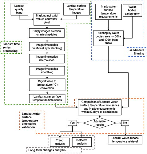
First, Landsat surface temperature (LST) images were processed by removing non-valid values according to the quality band, masking the water pixels, and creating empty images to replace the missing images. The time series composition was done by the layer stacking approach. It was then interpolated to fill in the missed values, smoothed to remove outliers, and converted to Celsius. Second, LWST time series were validated with field data to assess the degree of agreement once the data processing methodology had been applied. Finally, if a successful validation was obtained, trend and isotherm analyses would be carried out to study the long-term changes in WST (Figure 1).

Figure 1. Flow chart of the research process.

Study area

For lake selection, a minimum surface area of 50 hectares was established. This threshold helps prevent adjacency errors in the NIR region caused by nearby land surfaces and bottom reflectance during sensor acquisitions (Zibordi et al. 2014; Arias-Rodriguez et al. 2023). Additionally, this area size ensures an adequate number of pixels can be retrieved from image acquisition, based on the sensor’s spatial resolution of 30 × 30 meters, which will serve as the source of radiometric data. Thus, the size was determined according to the following criteria: (1) each water body must have at least three pixels on each side, (2) in situ data points must be at least one pixel away from the edge, to avoid land proximity influence, and (3) Each water body should have a safety margin to account for seasonal fluctuations of the water surface. This was obtained by comparing the Ministry for the Ecological Transition and the Demographic Challenge (MITECO) boundaries with high-resolution images from Google Maps.

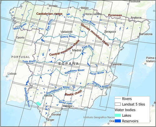
Then, an initial selection of inland waters in Spain with an area larger than 50 ha was done using the inland water boundaries from cartography supplied by the MITECO, water bodies with elongated shapes, e.g. dammed rivers, were excluded because their variability could affect the results. This was done using the elongation ratio equation (Re), which is the relationship between the area and the square of the length (Sukristiyanti et al. 2018). The preliminary selection yielded 325 water bodies, including 53 lakes (18 artificial, 23 natural and 12 heavily modified) and 272 reservoirs, all of them located in mainland Spain (Figure 2).

Figure 2. Location of the studied water bodies.

Input data

Landsat surface temperature data

The Landsat water surface temperature (LWST) data was obtained from the USGS Landsat surface temperature (LST) provisional product with a spatial resolution of 30 meters and a temporal resolution of 16 days. The LST was derived using Landsat 5 Thematic Mapper (TM), North American Regional Reanalysis (NARR) weather data, the Moderate Resolution Atmospheric Transmission (MODTRAN) model, and ASTER emissivity data (Malakar et al. 2018; Zanter 2021).

All the available LST data for peninsular Spain, 11,481 images in total, were downloaded from 1994 to 2011. Landsat 5 collection 2 level 2 scenes were downloaded in bulk from the EROS Earth Explorer website (https://earthexplorer.usgs.gov). Every image package included twelve output raster layers. The raster layers used in this research are surface temperature (ST) and pixel quality assessment (PIXELQA), which assigns each pixel a condition (clear terrain, water terrain, cloud shadow, or snow/ice) based on spectral information and confidence level (low, medium, and high).

Water surface temperature in situ measurements for landsat data validation

The water surface temperature data measured in the field provided by MITECO will be used to validate the Landsat water surface temperature time series. A total of 46,086 points providing surface temperature in degrees Celsius in 677 water bodies were obtained between 1994 and 2020.

Sampling was confined to water bodies with a surface area greater than or equal to 50 ha because smaller water bodies could not be studied with Landsat due to the image pixel size. In total, 36,105 sampling data points were preliminarily selected. Finally, only sampling points located more than 120 meters from the shore were selected by using the inland water boundaries from cartography supplied by MITECO because, although the surface temperature product has a spatial resolution of 30 meters, the original thermal band is 100 meters. In this way, the ground effect is removed as the pixel is resampled. The sampling data used for validation are 3,032 (Figure 3 and Table 1), located in 70 water bodies, of which 17 are lakes and 53 are reservoirs.

Figure 3. Available Landsat images and selected in situ surface temperature data per year.

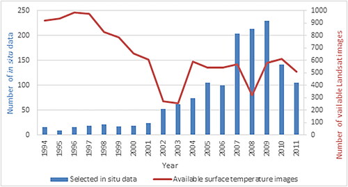
Table 1. Number of selected in situ points for every filtering process.

Filtering process	Number of in situ data	Number of water bodies
Initial	46086	677
In water bodies with surface area ≥ 50 ha	36105	432
Located more than 120 m from the shore	3032	70

Landsat water surface temperature time series processing

Data filtering

LST images were masked to null values according to the quality band (QA_PIXEL) to obtain standard values without clouds. Then, empty images were created to get images for missing dates and construct image data cubes representing evenly spaced time series associated to spatially aligned pixels. The water boundary was obtained based on quality band (QA_PIXEL) by using the ‘water with low sets’ class, which is used for masking surface temperature images.

Time series creation

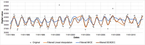
Subsequently, the LST image time series composition or data cube construction was carried out using the layer stacking approach. The imputation of missing values was carried out with the linear interpolation method. Three imputation methods were tested to determine which one was the most accurate and the least computationally expensive: lineal interpolation (Ponkina et al. 2021), the Multivariate Imputation by Chained Equations (MICE) (van Buuren and Groothuis-Oudshoorn 2011) and the Seasonally Decomposed Missing Value Imputation method (SEADEC) (Moritz and Bartz-Beielstein 2016) (Figure 4). By visual inspection, MICE was the least reliable method and linear interpolation and SEADEC got similar results with differences only in periods with more missing data (years 2002, 2003 and 2008). To quantify the difference between the linear interpolation and SEADEC methods, the general trend was calculated and compared (see the section ‘Water Surface Temperature Trend Analysis’) for five water bodies with varying trend levels distributed across the study area. The results showed a mean difference value of 0.0007 between the two methods. Consequently, the linear interpolation method was selected because the SEADEC method is computationally more expensive, especially considering the amount of data involved.

Figure 4. Comparison of imputation methods: Example with filtered time series.

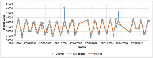
Then, smoothing with the Whittaker filter to eliminate outliers was done (Figure 5). The Whittaker smoother (Whittaker 1922) is a penalized least squares algorithm that minimizes fitting error and penalizes the roughness of the smooth curve. It can effectively balance the fidelity of the original time series and roughness of the fitted time series (Kong et al. 2019; Zeng et al. 2020; Liu et al. 2022).

Figure 5. Interpolation and filtering process example.

Conversion to celsius

Finally, given that LWST images are in scaled Kelvin values (SKV), it is necessary to convert them to degrees Celsius ($T(°C)$) to compare them with the field values. The following equations were used (Zanter 2021): (1) $$T(°K)=\mathit{\text{SKV}}\mathrm{ }\mathrm{*}\mathrm{ }0.00341802+149$$(1) (2) $$T(°C)=T(°K)-273.15$$(2)

At the end of the processing, a time series of water surface temperature was obtained for each water body for each available Landsat tile, so the tile with the most valid data was selected. Then, pixels that were classified as water throughout the whole time series were selected. Finally, 325 time series were obtained, given that water bodies with dry periods were discarded.

Landsat water surface temperature time series validation with in situ data

Because there was a lack of images during the studied period and the time series will be used to analyze long-term changes, they were validated to assess the performance of the processing methodology. So, the filtered in situ temperature measures for a three-day window of coincidence with the Landsat images were compared. A three-day time window was selected because there is a negative correlation between accuracy and the length of the time window (Zeng et al. 2023) and three-day windows have proven to be sufficient in previous studies (Schaeffer et al. 2018). The agreement was quantified by using the Pearson correlation coefficient and p-value to consider whether the correlation was statistically significant (Schaeffer, Seegers, et al. 2018; Baughman and Conaway 2021).

Water surface temperature trend analysis

Once the image data cube evenly representing the time series of water surface temperature had been obtained for every water body in the study, the general trend for each spatially aligned pixel from 1994 to 2011 was obtained. The trend analysis was done by fitting a linear least-square regression model as a function of time (Mahmoudi et al. 2019; Wang et al. 2021). The slope of the line indicates the positive or negative direction of the trend. The F test of the ANOVA regression was used to test the null hypothesis that the slope (regression coefficient) is null. Considering an alpha level of 0.1, if the p-value of the F-test statistic is less than the selected alpha level, the null hypothesis can be rejected (Wanishsakpong and McNeil 2016; Chambers and Hastie 1991; Mahmoudi et al. 2019).

A p-value and slope were obtained for every pixel from each water body, and the average of all pixels with significative slope within each water body was calculated and analyzed.

To compare the trends in water surface temperature with the surrounding air temperatures, daily mean data from all stations available at the Spanish State Meteorological Agency (AEMET) were downloaded, the trends were calculated by fitting a linear regression, and the resulting trend values were interpolated using the Inverse Distance Weighting (IDW) method (Tanır Kayıkçı and Zengin Kazancı 2016).

To quantify the rate of increase, the mean WST for each water body was determined, and the annual mean was calculated only for water bodies with a significant trend. The difference for each year was then calculated to obtain the mean difference.

Isotherm analysis

The spatial variation in the WST over time was studied with an isotherm-based method tested in the research of Wang et al. (2021). A total of three isotherms were created: 10 °C, 20 °C and 25 °C. A raster was created in the GIS software (ArcGIS Pro 3.1.2) by interpolating the mean WST of all studied water bodies every 16 days, so the calculated raster represents the hypothetical WST for each pixel, assuming all pixels represent water. To dismiss errors, none of the natural water bodies were included because of their high degree of variability. Finally, three different isotherms were calculated for each raster. If more than one isotherm was created for one temperature value, the longest isotherm was selected to calculate X (Longitude or East) and Y (Latitude or North) coordinates of its central point and the total length of the curve.

Once the central coordinates and length of the longest isotherms of temperatures 10 °C, 20 °C and 25 °C were obtained the seasonal behavior and the interannual changes or long-term trends were analyzed. To detect the long-term trend an analytical adjustment by regression was made by adjusting linear regression models as a function of time, confirming the significance of the slope of the straight line (Mahmoudi et al. 2019; Wang et al. 2021).

The data supporting the findings of this study are available from the corresponding author upon reasonable request.

Results and discussion

Landsat water surface temperature time series validation

After the Landsat time series processing, the time series were validated with a three-day window match-up for in situ points. Only data points with three or more coincidences were selected to compute the Pearson correlation coefficient. Finally, 341 coincidences were obtained in 23 in situ points in 20 inland water bodies (Figure 6). The Pearson correlation coefficient ranged from 0.60 to 0.98 with all p-values less than 0.1. In 87% of the cases, the p values were less than 0.05 (Table 2), which indicates a sufficiently significant correlation. This supports the use of remote sensing data in the analyses carried out.

Figure 6. Location of in situ data point coincident with landsat water surface temperature time series in a three-day window. The in situ identifier corresponds to Table 2.

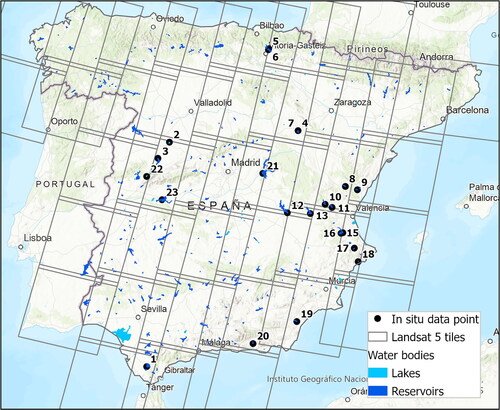
Table 2. Summary of agreement between landsat water surface temperature time series and in situ water temperature.

Id	Water body name	Field point code	Tiles	# of coincident data	Pearson	P-value
1	Barbate reservoir	AA00000750	201035	7	0,98	0,00
2	Riolobos reservoir	DURIO1	202031	5	0,93	0,02
3	Santa Teresa reservoir	DUTER1	202032	5	0,92	0,03
4	La Tranquera reservoir	EB00000553	200031	17	0,65	0,00
5	Ullivarri-Gamboa reservoir	EB00000827	201030	14	0,76	0,00
6	Ullivarri-Gamboa reservoir	EB00000829	201030	14	0,65	0,05
7	La Tranquera reservoir	EB0553-FQ	200031	5	0,97	0,01
8	Arenós reservoir	JU06140034	199032	9	0,75	0,02
9	Sichar reservoir	JU06150028	198032	10	0,98	0,00
10	Benagéber reservoir	JU06660017	199032	7	0,65	0,09
11	Loriguilla reservoir	JU06660020	199032	9	0,67	0,05
12	Alarcón reservoir	JU06910006	200032	9	0,82	0,01
13	Contreras reservoir	JU06930008	199033	14	0,63	0,02
14	Tous reservoir	JU07460013	199033	16	0,60	0,01
15	Escalona reservoir	JU07690008	199033	61	0,63	0,00
16	Escalona reservoir	JU07690041	199033	18	0,67	0,00
17	Beniarrés reservoir	JU08210023	198033	19	0,96	0,00
18	Amadorio reservoir	JU08470015	198033	14	0,97	0,00
19	Cuevas de Almanzora reservoir	MA1014B001	199034	9	0,94	0,00
20	Benínar reservoir	MA1043B006	200034	21	0,96	0,00
21	Buendía reservoir	TA56201002	200032	38	0,63	0,00
22	Baños reservoir	TACC576996	202032	9	0,81	0,01
23	Valdecañas reservoir	TACC652014	202032	11	0,85	0,00

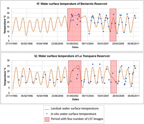
The lack of images between 2002 and 2003 and in 2008 affects the LWST time series behavior, especially because the non-available images correspond to winter periods (Figure 7). Despite the underestimation of LWST in 2002, 2003, and 2008 with respect to in situ values, the accuracy obtained is acceptable.

Figure 7. Landsat and in situ water surface temperature time series. (a) Beniarrés reservoir, point code: JU08210023, slope: 0.0053 (p 0.03) and (b) La tranquera reservoir, point code: EB00000553, slope: 0.0071 (p 0.002).

The overall performance of the time series processing methodology of the LST product was achieved for all points with a Pearson correlation coefficient and significative (p < 0.1) in all cases. If there is a correlation between LWST time series and in situ surface temperature, the LWST time series could be sufficient for determining historical seasonal trends and assessing the inter-annual variability of water bodies. This is similar to results in previous studies in which authors concluded, that due to the high performance in open water pixels, Landsat satellite time series can supplement traditional in situ sampling by providing data for most water bodies for an extended period (Schaeffer et al. 2018; Duan et al. 2020; Baughman and Conaway 2021).

Water surface temperature trend analysis

To determine whether the slope was significant linear least-square regression was done for all the water surface temperature time series for all pixels in every water body.

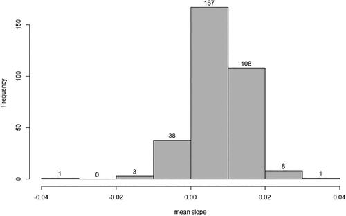
Most pixels, 70.13%, have a statistically significant positive trend (p < 0.1), 5.66% have a statistically significant negative trend, and 24.21% have no significant trend. The average of all pixels with a significant slope was 0.0072, which means that the WST increased in the 18-year study period, from 1994 to 2011. The mean significant slope for all pixels in each water body shows that 87% of water bodies have a positive mean slope (Figure 8). This means that the temperature has increased in those water bodies during the study period.

Figure 8. Mean of significant slope for each water body.

This is consistent with trends in the temperature of inland water bodies in other countries around the world. Wang et al. (2021) concluded that the temperature of lakes in China has shown an upward trend from 2000 to 2010; Schneider et al. (2009) found that lakes in California and Nevada (North America) had a rapid warming trend from 1991 to 2008; Aranda et al. (2021) analyzed monthly, seasonal and annual surface temperature trends in 14 Chilean lakes between 2000 and 2016 period with the results showing that 12 of them presented a statistically significant increase in surface temperature; Dokulil (2014) found that most inland waters in Europe showed a warming trend between 1960 and 2010; and Schneider and Hook (2010, 2012) concluded that the surface temperatures of 169 of the largest inland water bodies worldwide have been increasing with the greatest warming in the middle and high latitudes of the Northern Hemisphere, and particularly in Northern Europe.

The results presented in this paper show that this warming trend represents an average of +0.037 °C per year in water bodies with a significant trend, which means a total of +0.592 °C over the entire study period. These results are consistent with those obtained by O’Reilly et al. (2015) for the whole world (+0.034 °C per year) and by Woolway et al. (2020a) for Europe (+0.035 °C per year). However, they are much higher than those of Virdis et al. (2020) for Sardinia (+0.01 °C per year), and considerably lower than those estimated by Schneider and Hook (2010) for Eastern Europe (+0.06 °C per year). The differences can be explained by the high spatial variability that WST trends can present as well as variations in the study periods. For example, Sardinia is a small island in the central Mediterranean Sea, and its climatic conditions are very different from those of the Iberian Peninsula.

In this study area, the WST trend distribution (Figure 9) is highly irregular due to its complicated orography and the diversity of climatic regions.

Figure 9. Daily mean air temperature trend interpolation (hatch) in peninsular Spain and significative WST mean slope for each water body (points). Only water bodies with more than 60% of pixels with significant slope are shown.

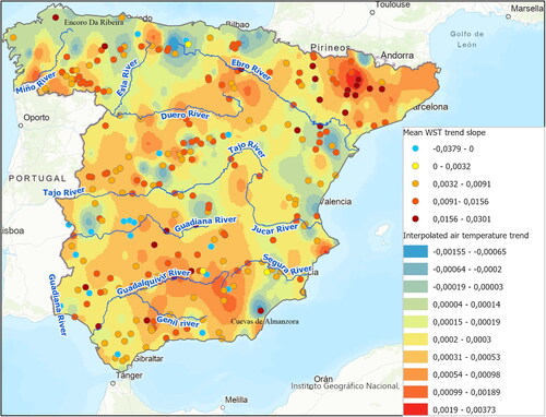
There is a pronounced warming trend in the water bodies of the Ebro River depression, located in the southern part of the Pyrenees. The warming trends in the Guadalquivir River basin are somewhat more variable and dispersed (Figure 9). These depressions are situated at altitudes of 200 and 100 meters, respectively, and feature a ‘continentalized Mediterranean with warm summers’ climate in the first one, and a ‘warm inland Mediterranean’ climate in the second, with both areas partial exhibiting an ‘arid Mediterranean’ climate (Instituto Geográfico Nacional, no date).

On the other hand, there are also elevated warming trends in high-altitude areas, such as the Montes de León (between the Miño and Esla rivers), as well as in the Cantabrian Range and the Central Mountain Chain in the middle part of the peninsula (see Figure s 2 and 9). These areas have altitudes ranging from 2,188 to 2,650 m above sea level (ASL), so water bodies that are geographically very close may experience different climates, e.g. a ‘subhumid continentalized Mediterranean’ climate, a ‘mountain’ climate, or a ‘transitional oceanic’ climate.

The trends are less pronounced on the northern plateau, which is situated at an altitude of 750 m ASL and experiences a ‘continentalized Mediterranean with cold winters’ climate. In contrast, the WST trends in water bodies on the southern plateau of the peninsula are much more varied. This region, with a slightly lower altitude (600 m ASL), falls within the ‘continentalized Mediterranean with warm summers’ and ‘Mediterranean inland warm’ climate zones. Here, water bodies exhibit a wide range of warming trends, some of which show a significant tendency to warm, some a moderate trend, and a few with hardly any tendency at all.

The results indicate a clear warming trend in the water masses of these areas. While this trend cannot be directly attributed to altitude or climate alone, it is likely to be influenced by a combination of climatic and other factors. These include local characteristics (O'Reilly et al. 2015), altitude and geographical position (Stefanidis et al. 2022), and solar radiation (Woolway et al. 2020).

Generally, the WST trend spatial patterns and air temperature trends coincide (Schneider and Hook 2010; Woolway et al. 2020; Wang et al. 2021). Our results show this relationship, particularly in the Ebro and Guadalquivir river depressions. However, there are zones where water bodies appear to warm more than the surrounding air (Austin and Colman 2007; Schneider and Hook 2010; O'Reilly et al. 2015). In Spain, this effect is observed at several locations across the study area. In some cases, an inverse relationship occurs; water bodies with high warming tendencies are situated in environments with negative air temperature trends. Examples of this include the Cuevas de Almanzora reservoir in the Southeast and the Encoro Da Ribeira reservoir in the Northwest of the peninsula, and several water bodies south of the Ebro River (Figure 9). This local variability could be explained by the greater influence of several combined elements in the so-called atmospheric circulation modes (Hernández et al. 2015) or by some other element, such as a strong altitudinal gradient (Sánchez et al. 2022) resulting from the complex peninsular orography.

The most significant warming trends were observed in the southern part of the peninsula trends become less pronounced in the central plateau to the north. However, there are strong warming trends further north, in the Northeastern (Pyrenees) and Northwest (Galicia) (Figure 10). The coastal influence is evident in both air temperature and WST trends on the East–West axis (Figures 9 and 10). In the East, the Mediterranean Sea appears to soften the warming trend that is occurring in the interior areas, but to the west is a cluster of water bodies with negative trends, indicating a cooling between 1994 and 2011, which may be due to the influence of fresh and humid Atlantic winds that penetrate the area through the Guadiana and Tajo depressions (García Vega and García de Pedraza 1991) (Figure 10).

Figure 10. Interpolated mean WST trend in peninsular Spain with IDW method.

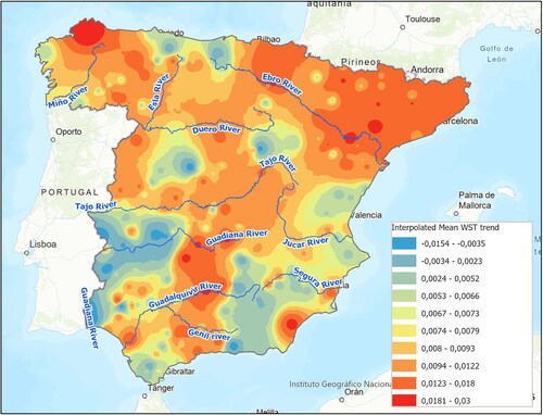
This outcome agrees with the global findings revealing increased warming in water bodies in temperate regions of the Northern Hemisphere (Schneider and Hook 2010; Piccolroaz et al. 2020), increasing warming trends in the southwest northeastern Europe (Lieberherr and Wunderle 2018), and in Mediterranean lakes (Virdis et al. 2020).

However, more research is needed to fully understand the warming processes in the Iberian Peninsula water bodies, because, although they seem to be influenced by global factors such as the increasing trend in air temperature associated with climate change (del Río et al. 2011; Ríos-Cornejo et al. 2015), there are other more local influences such as geomorphology, elevation, and climate that need to be analyzed.

Isotherm analysis

Seasonal variation

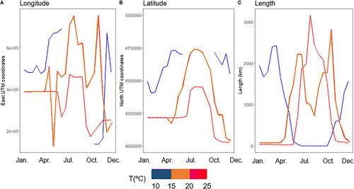
Low temperatures occur in the Iberian Peninsula at latitudes above 4,350,000 N, meaning the water bodies in Andalusia maintain temperatures above 10 °C throughout the year. During spring, between February and June, the 10 °C isotherm move from the water bodies located in the peninsular center to those located further north, gradually disappearing (Figure 11b). There is a western movement at the end of spring and during the autumn. On the other hand, the number of water bodies with10 °C or lower temperatures increases between October and March, after which temperatures rise until June, when no water bodies in the Iberian Peninsula have 10 °C or less (zero length of the 10 °C isotherm, Figure 11c).

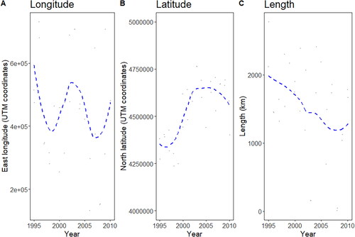
Figure 11. Seasonal changes in a) longitude of the midpoint, (b) latitude of the midpoint, (c) length of the isotherms 10 °C, 20 °C and 25 °C inland WST in Spain during year 2010.

This WST seasonal spatial pattern may be closely related to air temperature (Alvarez Cobelas & Rojo García-Morato, 2021), but it is even more strongly associated with land surface temperature (LST). On the peninsula, land surface warming begins in April in the East and decreases between September and October. Temperatures decrease earlier in the Northwest (Khorchani et al. 2018).

The 25 °C isotherm generally appears stable in water bodies in the south and part of the center region of the peninsula until summer (June), after which they are further north, remaining stable at those latitudes until September. This displacement occurs because a range of higher temperatures affects the water bodies in these territories. In October, the reverse movement occurs, bringing temperatures of 25 °C back to the water bodies of the southern peninsula (Figure 11b). There are areas of the peninsula in which water temperatures reach 25 °C, even in the autumn months, e.g. November 2010 (Figure 12). However, during autumn, winter and spring very few water bodies on the peninsula reach 25 °C. Their number increases rapidly from June to August, when it decreases again until the end of October (length of the isotherm 25 °C in Figure 11c). The longitudinal movement of the 25° isotherm has a similar pattern of latitude, it increases in summer and rapidly decreases in early autumn (Figure 11a).

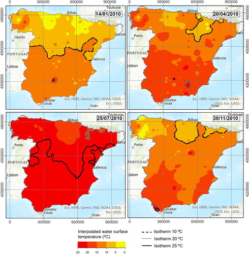
Figure 12. Location of the isotherms 10 °C, 20 °C and 25 °C inland WST in different seasons during the year 2010.

As previously mentioned, the warming of water bodies parallels that of the LST. The heat moves northeast through the Guadalquivir depression, reaching 25 °C WST in most of the peninsula, but not the Mediterranean and the Cantabrian coasts. The Ebro basin is characterized by a perpendicular pattern, that is warming towards the northwest from its mouth in the Mediterranean. This area has certain water bodies outside the pattern, influenced by the Pyrenees’ orography.

Regarding intermediate temperatures (20 °C), the largest number of water bodies with this temperature occurs in the months of May and October, with a minimum in August coinciding with the greatest presence of water bodies at 25 °C. During the summer months, in which there are no water bodies at 10 °C, the 20 °C isotherm takes its place (Figure 11b) occupying positions further north than the 25 °C isotherm (July 2010, Figure 12).

The seasonal spatial distribution of the WST shows practically the same pattern in all seasons (Figure 12) – South–North gradient with localized areas of lower temperatures. In winter (01/14/2010 in Figure 12), the water bodies in the southern half of the peninsula have temperatures between 10 and 15 °C, while most in the northern half range between 5 and 10 °C. Two localized areas have water temperatures below 5 °C, influenced by the Pyrenees and Cantabrian mountain ranges and the Cantabrian Sea. A similar pattern occurs in spring, but with each area experiencing a WST higher range (04/20/2010 in Figure 12). The autumn shows a similar distribution (11/30/2010 in Figure 12), but in this case, the influence of the Betic System in the southeast of the peninsula is evident. In summer, almost all water bodies have temperatures of 25 °C or higher, with only a few having lower temperatures of about 20 °C. The areas with lower temperature ranges are practically the same in all seasons (<5 °C in Winter, <10° C in Spring and Autumn, <20 °C in Summer, see Figure 12).

There are significant spatial and seasonal differences in WST throughout peninsular Spain. This variability appears to be strongly related to air temperature or LST and its associated components such as vegetation cover (Khorchani et al. 2018), although the influence of other local components, such as those derived from the country’s complex orography (altitude, slopes, very local microclimates, etc.) must also be considered (Sánchez et al. 2022). In some cases, the lakes of the peninsula show greater sensitivity to variations in atmospheric circulation modes (ACM) than to individual local meteorological variables (Hernández et al. 2015).

Long term tendencies

To study interannual changes by month in the 10 °C, 20 °C and 25 °C isotherms, the trend slope and p-value of longitude and latitude coordinates and length for each isotherm was analyzed for every month between 1994 and 2011 (Table 3). The results show that the 10 °C isotherm has a statistically significant (p < 0.1) negative trend slope in September, October and December for X-central coordinate (or longitude).

Table 3. Trend slope and p-value of longitude and latitude coordinates and length of isotherms 10ºC, 20ºC and 25ºC for each month from 1994 to 2011.

Month	Slope Isotherm 10ºC	p-value	Slope Isotherm 20ºC	p-value	Slope Isotherm 25ºC	p-value
Longitude
January	−47.86206	0.98	−1544.549	0.67	−991.5659	0.64
February	−1903.188	0.54	143.6676	0.90	0	0.91
March	−2021.019	0.25	4686.336	0.15	453.5949	0.44
April	−605.9494	0.86	3988.531	0.11	2782.055	0.25
May	−3527.173	0.43	2287.408	0.31	6071.056	0.02*
June	0	0.74	−1641.126	0.34	2091.991	0.59
July	0	0.86	−1475	0.55	−998.4874	0.19
August	0	0.93	2057.775	0.37	281.6293	0.67
September	−12601.61	0.01*	−983.1453	0.39	−1418.796	0.61
October	−7685.64	0.05*	1943.151	0.16	−430.9965	0.83
November	−1572.138	0.78	−3712.518	0.29	−7730.225	0.09*
December	−5325.773	0.06*	−3741.66	0.23	−1783.632	0.59
Latitude
January	9793.491	0.005*	−2685.004	0.18	−2938.565	0.28
February	9237.682	0.008*	1304.762	0.52	−2611.667	0.49
March	3640.95	0.14	1291.38	0.32	7636.204	0.11
April	−875.6807	0.28	690.4239	0.79	2933.916	0.34
May	−116.7445	0.45	804.7101	0.78	−1265.329	0.42
June	0	0.45	959.3492	0.34	−1808.512	0.21
July	0	0.93	−459.032	0.44	522.0772	0.85
August	0	0.52	699.2438	0.32	2322.054	0.19
September	−1068.291	0.37	2641.068	0.03*	3410.819	0.10*
October	0	1	3384.899	0.23	−1309.704	0.32
November	722.7777	0.55	311.2409	0.73	−4613.935	0.07*
December	7534.344	0.02*	−1253.506	0.63	−2189.86	0.38
Length
January	−13.25814	0.35	−0.5007776	0.92	1.076808	0.38
February	−9.159196	0.56	9.300592	0.10*	0.7455181	0.70
March	−19.82289	0.12	1.308572	0.42	1.365169	0.28
April	−7.52237	0.42	−6.926845	0.57	−1.432626	0.57
May	1.009959	0.45	2.650647	0.88	−14.68862	0.05*
June	0	0.91	−14.79569	0.35	−9.68697	0.51
July	0	0.79	−6.954177	0.49	10.85281	0.31
August	0	0.68	−20.1464	0.01*	9.389652	0.10*
September	−4.609443	0.05*	−18.00391	0.14	8.977678	0.48
October	−15.42589	0.001*	−0.2185724	0.97	0.282008	0.97
November	−47.82879	0.001*	6.059229	0.63	−2.261955	0.52
December	−37.02459	0.009*	−1.693451	0.73	−2.243785	0.38

*Statistically significant p-value.

This suggests that over the studied years, the 10 °C isotherm has been shifting westward. Additionally, its central Y coordinate (latitude) shows a significant positive trend from December to February, while the isotherm is also becoming shorter. This implies that between 1994 and 2011, there were fewer water bodies with a temperature of 10 °C, and these bodies of water were located further north.

The 25 °C isotherm does not show clear a movement pattern. In May it moved eastward, in September it moved northward, and in November it moved to the south-west. What it does show is that in August, the month where the land surface temperature is highest in the Iberian Peninsula (Figure 12), the length of the 25 °C isotherm has a significant positive trend.

In contrast, the 20 °C isotherm shows few significant trends. At the end of summer (September), it tends to move northward. There is a significant trend for it to decrease in length in August, but there is little tendency for it to increase in length in February (Table 3).

This shows: (1) a greater northward trend and decreasing length temperatures of 10° C in winter and (2) at the end of summer, the 20° C isotherm tends to remain further north and its length decreases (3) the 25° C isotherm increased in length, which means that in 2011 there were more water bodies with a surface temperature of 25° C.

Illustrative months were selected to visualize the interannual movements and lengths of WST 10° C and 25° C isotherms, considering the months when each isotherm has significative trend in central coordinates or length (Table 3). Assuming December as the representative month of WST 10° C, the spatial changes from 1994 to 2011 were studied using the midpoint of the longest 10° C isotherm. As can be seen from Figures 13 and 15, the isotherm gradually shifted northward by approximately 4,625,000 North UTM (latitude) coordinate, until 2007, then it started to move southward about 4,375,000 N. In the longitude direction, the central point shows a cycle movement with no big movements, first westward about 400,000E before 1997, then gradually moved eastward by about 550,000 East UTM (longitude) coordinate and repeated the same movement to the coordinate 500,000 E in 2011. The length of the January 10° isotherm decreased from 2,400 km in 1994 to 1,900 km in 2011.

Figure 13. Interannual changes in a) longitude of the midpoint, (b) latitude of the midpoint, (c) length of isotherm 10 °C in Spain inland water bodies in December from 1994 to 2011.

In the case of WST 25 °C, the length and midpoint of the longest August 25 °C isotherm were analyzed to study interannual movement (Figures 14 and 15). Although the central coordinate of the 25 °C isotherm did not move much to the north (from coordinate 4,400,000 N in 1994 to coordinate 4,500,000 N in 2011) or to the east (from coordinate 450,000E in 1994 to coordinate 460,000E in 2011), its length varies from 1,750 km in 1994 to 2,000 km in 2011.

Figure 14. Interannual changes in a) longitude of the midpoint, (b) latitude of the midpoint, (c) length of isotherm 25 °C in Spain inland water bodies in August from 1994 to 2011.

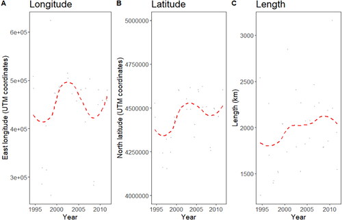
Figure 15. Location of the isotherms 10 °C, 20 °C and 25 °C WST in 1995, 2001 and 2009.

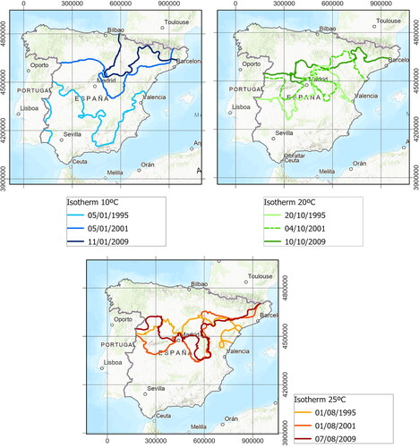
Thus, while the 10 °C isotherm decreased in length and its central point moved towards the north of the peninsula above 4,625,000 N in 2011, the 25 °C isotherm increased in length and its central point has also moved towards the north, reaching 4,500,000 N in 2011.

The 20 °C isotherm exhibits a distribution pattern that combines characteristics of the previous ones. It shifts northward, though less pronouncedly than the 10 °C isotherm, while extending in length similarly to the 25 °C isotherm, folding within its zone of influence (slightly to the north-central area of the peninsula) (Figure 15).

In summary, by the end of the period from 1994 to 2011, an increasing number of water bodies had reached temperatures of 25 °C. However, this temperature is not reached by water bodies located in the northern region of the peninsula. As temperatures decline in autumn, there is also a growing prevalence of water bodies with relatively warm temperatures (20 °C) situated farther north that at the beginning of the period. During winter, there was a noticeable decrease in the number of water masses that cooled with temperatures dropping to 10 °C or below. Additionally, these cool water bodies were also positioned considerably farther north that in 1994.

The outcomes agree with several authors who studied interannual variations of WST and found that the most visible trend and pattern changes occurred during the coldest seasons. Niedrist et al. (2018) studied a 44-year time series of water temperature from a small mountain lake in Austria and observe a significant long-term warming trend. However, but this occurred only from August to December with a significant autumn/winter warming effect of lake water together with an increasing intensity of temperature fluctuations in this seasonally ice-covered mountain lake, suggesting that current broad scale estimates of climate change impacts on lakes, based on summer temperature measurements and surface layers, do not fully reflect the effect of climate change. Woolway et al. (2019) investigated the changes in annual minimum surface water temperature in eight European lakes (one in Ireland, five in the UK, one in Austria and one in Switzerland) and found that between 1973 and 2014, the annual minimum lake surface temperature had increased at an average rate of + 0.35 °C per decade, which is comparable to the rate of summer average lake surface temperature change during the same period (+ 0.32 °C per decade) As a result of the rapid warming of annual minimum lake surface temperatures, some of the lakes studied no longer reach important minimum winter surface temperature thresholds, with complex and significant potential implications for the lakes and the ecosystem services they provide. Öğlü et al. (2020) determined long-term trends and detected changes in the frequency of extreme events in the surface water temperature of Lake Peipsi in Russia between 1950 and 2018. Their results showed that, although the average surface temperature had not increased significantly on an annual basis since 1950, it rose rapidly in the winter season during the last decade. Aguilar-Lome et al. (2021) evaluated the space-temporal variation of the water surface temperature of Lake Titicaca in the Central Andes during the period 2000 to 2020 and found that there is a general increasing trend of the average LWST during the coldest time (winter) of the year. Huang et al. (2023) simulated lake surface water temperature between 1979 and 2018 for 91 large lakes across China. Most these lakes showed significant warming trends with a higher rate in winter and spring than in summer and autumn.

In the Mediterranean geographical setting, Virdis et al. (2020) examined 24 lakes on the island of Sardinia between 1999 and 2018. They observed a warming trend of 0.01 °C per year, predominantly occurring during winter. Conversely, there was a tendency towards cooling during the summer months.

These results are critical for the ecology of lakes and continental water bodies. For example, freshwater biodiversity can be negatively impacted because communities at sites with faster rates of warming had fewer gains in taxon richness, functional richness, and abundance (Haase et al. 2023). Regarding freshwater fauna, many fish species have limited capacity to disperse in response to new environmental conditions (Carosi et al. 2023), so their situation is likely to worsen, as rising temperatures could encourage an increase in invasive fish species (Woodward et al. 2010).

On the other hand, the increase in water temperature affects the growth of phytoplankton (Tewari 2022), and many species of cyanobacteria prefer warmer temperatures (Glibert 2020), with some thriving above 25 °C (Paerl and Huisman 2009). Additionally, the complex dynamics in the water column and between species can lead to nonlinear effects, so the results could be more severe than initially expected (Jöhnk et al. 2008; Griffith and Gobler 2020). From the periodic data obtained in this research, it is possible to derive models (Zhu et al. 2022; Piccolroaz et al. 2024) that enable the daily study of temperature dynamics in these bodies of water and their evolution in the context of climate change.

Conclusions

This research shows that during the period from 1994 to 2011 there was an average warming of water bodies of +0.037 °C per year. This is similar in magnitude to that found in large areas of the world and Europe, but this trend is distributed variably across the entire peninsular territory.

Differences appear to be associated with air temperature and land surface temperature but, in certain areas, altitude has a greater influence, with the water bodies of the mountain Montes de León, Cantabrian Range, and Central Mountain Chain showing more pronounced trends. The influence of southwest–northeast Atlantic winds on the cooling of a group of water bodies in the Guadiana basin was also revealed.

The trends have not been fully explained, so the influence of factors such as climate and other local conditions such as elevation, geomorphology, winds, even vegetation cover, or their combination, must be studied.

Throughout the period from 1994 to 2011, the long-term warming trend differed according to the seasons. There was an increase in the number of water bodies with high temperatures during the summer, despite no geographical displacement on the peninsula. In autumn, there were more water bodies with intermediate temperatures and they were situated farther north than at the beginning of the period. During winter and spring, water bodies with cold temperatures were located further north and were less numerous.

Regarding the implemented methodology, it has been demonstrated that the Landsat 5 surface temperature product can be successfully applied to describe a historical series of temperature for continental water bodies in Spain.

This work has a temporal limitation, as it analyzes a relatively short time span to study the phenomenon of warming in inland water bodies. However, applying the developed methodology to other sensors will allow extending the study period, expanding it to the present. Clearly, other study field areas can benefit from the application of this methodology. However, there is potential for improvement by, e.g. combining data from different sources and interpolation processes to reduce data gaps and achieve a more robust and adjusted time series.

In the present era of global climate change, in which temperature plays an important role in freshwater bodies ecology, enhancing our comprehension of the warming mechanisms impacting these ecosystems is imperative. Continuous long-term monitoring, covering wide spatial and temporal scopes, is essential to safeguard their sustainability and ensure the continuity of the ecosystem services they offer.

In that regard, we aim for this paper to be a valuable and practical tool in achieving that goal.

Acknowledgments

We thank the ©Ministerio para la Transición Ecológica y el Reto Demográfico (MITECO) for providing us water surface temperature field data. This research did not receive any specific grant from funding agencies in the public, commercial, or not-for-profit sectors. There are no relevant financial or non-financial competing interests to report.

Disclosure statement

No potential conflict of interest was reported by the authors.

References

- Aguilar-Lome J, Soca-Flores R, Gómez D. 2021. Evaluation of the Lake Titicaca’s surface water temperature using LST MODIS time series (2000–2020). J South Am Earth Sci. 112:103609. doi: 10.1016/j.jsames.2021.103609.[Mismatch]
- Alcântara EH, Stech JL, Lorenzzetti JA, Bonnet MP, Casamitjana X, Assireu AT, Novo EMLdM 2010. Remote sensing of water surface temperature and heat flux over a tropical hydroelectric reservoir. Remote Sens Environ. 114(11):2651–2665. doi: 10.1016/j.rse.2010.06.002.
- Alvarez Cobelas M, Rojo García-Morato C. 2021. That twenty years is nothing for gravel-pit limnology. Limnetica. 40(1):169–187. doi: 10.23818/limn.40.12.
- Aranda A, Rivera-Ruiz D, Rodríguez-López L, Pedreros P, Arumí-Ribera J, Morales-Salinas L, Fuentes-Jaque G, Urrutia R. 2021. Evidence of climate change based on lake surface temperature trends in south central Chile. Remote Sens. 13(22):4535. doi: 10.3390/rs13224535.
- Arias-Rodriguez LF, Tüzün UF, Duan Z, Huang J, Tuo Y, Disse M. 2023. Global water quality of inland waters with harmonized landsat-8 and sentinel-2 using cloud-computed machine learning. Remote Sens. 15(5):1390. doi: 10.3390/RS15051390/S1.
- Armstrong JB, Fullerton AH, Jordan CE, Ebersole JL, Bellmore JR, Arismendi I, Penaluna B, Reeves GH. 2021. The importance of warm habitat to the growth regime of cold-water fishes. Nat Clim Chang. 11(4):354–361. doi: 10.1038/s41558-021-00994-y.
- Austin JA, Colman SM. 2007. Lake Superior summer water temperatures are increasing more rapidly than regional temperatures: a positive ice-albedo feedback. Geophys Res Lett. 34(6):L06604. doi: 10.1029/2006GL029021.
- Baughman CA, Conaway JS. 2021. Comparison of historical water temperature measurements with Landsat analysis ready data provisional surface temperature estimates for the Yukon River in Alaska. Remote Sens. 13(12):2394. doi: 10.3390/rs13122394.
- Brönmark C, Hansson LA. 2002. Environmental issues in lakes and ponds: current state and perspectives. Envir Conserv. 29(3):290–307. doi: 10.1017/S0376892902000218.
- Carosi A, Lorenzoni F, Lorenzoni M. 2023. Synergistic effects of climate change and alien fish invasions in freshwater ecosystems: a review. Fishes. 8(10):486. doi: 10.3390/fishes8100486.
- Chambers JM, Hastie TJ. 1991. Linear Models. Statistical Models in S. London: Chapman & Hall. doi: 10.1201/9780203738535.
- Chao Rodríguez Y, el Anjoumi A, Domínguez Gómez JA, Rodríguez Pérez D, Rico E. 2014. Using Landsat image time series to study a small water body in Northern Spain. Environ Monit Assess. 186(6):3511–3522. Available at: doi: 10.1007/S10661-014-3634-8/FIGURES/11.
- Dekker AG, Hestir EL. 2012. ‘Evaluating the feasibility of systematic inland water quality monitoring with satellite remote sensing’, publications.csiro.au [Preprint]. Available at: https://publications.csiro.au/rpr/download?pid=csiro:EP117441&dsid=DS10 (Accessed: 1 April 2023).
- del Río S, Herrero L, Pinto-Gomes C, Penas A. 2011. Spatial analysis of mean temperature trends in Spain over the period 1961–2006. Global Planet Change. 78(1-2):65–75. doi: 10.1016/j.gloplacha.2011.05.012.
- Dokulil MT. 2014. Impact of climate warming on European inland waters. IW. 4(1):27–40. doi: 10.5268/IW-4.1.705.
- Dokulil MT, de Eyto E, Maberly SC, May L, Weyhenmeyer GA, Woolway RI. 2021. Increasing maximum lake surface temperature under climate change. Clim Change. 165(3-4):1–17. doi: 10.1007/S10584-021-03085-1/FIGURES/6.
- Dörnhöfer K, Oppelt N. 2016. Remote sensing for lake research and monitoring – recent advances. Ecol Indic. 64:105–122. doi: 10.1016/j.ecolind.2015.12.009.
- Duan SB, Li ZL, Zhao W, Wu P, Huang C, Han XJ, Gao M, Leng P, Shang G. 2020. Validation of Landsat land surface temperature product in the conterminous United States using in situ measurements from SURFRAD, ARM, and NDBC sites. Int J Digital Earth 14(5): 640–660. doi: 10.1080/17538947.2020.1862319.
- García Vega C, García de Pedraza L. 1991. ‘Contrastes meteorológicos en la península ibérica: cuenca atlántica frente a zona mediterránea’, Repositorios AEMET [Preprint]. https://repositorio.aemet.es/bitstream/20.500.11765/905/1/contrastes_cal92.pdf (Accessed: 1 June 2024).
- Glibert PM. 2020. Harmful algae at the complex nexus of eutrophication and climate change. Harmful Algae. 91:101583. doi: 10.1016/J.HAL.2019.03.001.
- Griffith AW, Gobler CJ. 2020. Harmful algal blooms: a climate change co-stressor in marine and freshwater ecosystems. Harmful Algae. 91:101590. doi: 10.1016/J.HAL.2019.03.008.
- Haase P, Bowler DE, Baker NJ, Bonada N, Domisch S, Garcia Marquez JR, Heino J, Hering D, Jähnig SC, Schmidt-Kloiber A, et al. 2023. The recovery of European freshwater biodiversity has come to a halt. Nature. 2023 620(7974):582–588. doi: 10.1038/s41586-023-06400-1.
- Hernández A, Trigo RM, Pla-Rabes S, Valero-Garcés BL, Jerez S, Rico-Herrero M, Vega JC, Jambrina-Enríquez M, Giralt S. 2015. Sensitivity of two Iberian lakes to North Atlantic atmospheric circulation modes. Clim Dyn. 45(11-12):3403–3417. doi: 10.1007/S00382-015-2547-8/TABLES/5.
- Hestir EL, Brando VE, Bresciani M, Giardino C, Matta E, Villa P, Dekker AG. 2015. Measuring freshwater aquatic ecosystems: the need for a hyperspectral global mapping satellite mission. Remote Sens Environ. 167:181–195. doi: 10.1016/j.rse.2015.05.023.
- Huang L, Wang X, Yan Y, Jin L, Yang K, Chen A, Zheng R, Ottlé C, Wang C, Cui Y, et al. 2023. Attribution of lake surface water temperature change in large lakes across China over past four decades. JGR Atmospheres. 128(21): e2022JD038465. doi: 10.1029/2022JD038465.
- Huang Y, Liu H, Hinkel K, Beck R, Yu B, Wu J. 2015. Analysis of water temperature variability of Arctic lakes using Landsat-8 data. International Geoscience and Remote Sensing Symposium (IGARSS), 2015-November, pp. 2501–2503. doi: 10.1109/IGARSS.2015.7326318.
- Instituto Geográfico Nacional. (no date) El clima en España. https://www.ign.es/espmap/mapas_clima_bach/pdf/Clima_Mapa_1_2texto.pdf. (Accessed: 1 June 2024).
- Jöhnk KD, Huisman JEF, Sharples J, Sommeijer BEN, Visser PM, Stroom JM. 2008. Summer heatwaves promote blooms of harmful cyanobacteria. Global Change Biol. 14(3):495–512. doi: 10.1111/j.1365-2486.2007.01510.x.
- Khorchani M, Martin-Hernandez N, Vicente-Serrano SM, Azorin-Molina C, Garcia M, Domínguez-Duran MªA, Reig F, Peña-Gallardo M, Domínguez-Castro F. 2018. Average annual and seasonal Land Surface Temperature, Spanish Peninsular. J Maps. 14(2):465–475. doi: 10.1080/17445647.2018.1500316.
- Klein I, Dietz AJ, Gessner U, Galayeva A, Myrzakhmetov A, Kuenzer C. 2014. Evaluation of seasonal water body extents in Central Asia over the past 27 years derived from medium-resolution remote sensing data. Int J Appl Earth Obs Geoinf. 26(1):335–349. doi: 10.1016/j.jag.2013.08.004.
- Kong D, Zhang Y, Gu X, Wang D. 2019. A robust method for reconstructing global MODIS EVI time series on the Google Earth Engine. ISPRS J Photogramm Remote Sens. 155:13–24. doi: 10.1016/j.isprsjprs.2019.06.014.
- Lieberherr G, Wunderle S. 2018. Lake surface water temperature derived from 35 years of AVHRR sensor data for European lakes. Remote Sens. 10(7):990. doi: 10.3390/rs10070990.
- Liu X, Ji, L, Zhang C, Liu Y. 2022. A method for reconstructing NDVI time-series based on envelope detection and the Savitzky-Golay filter. 15(1):553–584. Available at: doi: 10.1080/17538947.2022.2044397.
- Mahmoudi P, Mohammadi, M, Daneshmand H. 2019. Investigating the trend of average changes of annual temperatures in Iran. Int J Environ Sci Technol. 16(2):1079–1092. doi: 10.1007/s13762-018-1664-4.
- Malakar NK, Hulley GC, Hook SJ, Laraby K, Cook M, Schott JR. 2018. An operational land surface temperature product for landsat thermal data: methodology and validation. IEEE Trans Geosci Remote Sens. 56(10):5717–5735. doi: 10.1109/TGRS.2018.2824828.
- Moritz S, Bartz-Beielstein T. 2016. imputeTS: time Series Missing Value Imputation in R. R package version 1.7 [Preprint].
- Moss B. 2012. Cogs in the endless machine: lakes, climate change and nutrient cycles: a review. Sci Total Environ. 434:130–142. doi: 10.1016/J.SCITOTENV.2011.07.069.
- Niedrist GH, Psenner R, Sommaruga R. 2018. Climate warming increases vertical and seasonal water temperature differences and inter-annual variability in a mountain lake. Clim Change. 151(3-4):473–490. doi: 10.1007/S10584-018-2328-6/FIGURES/5.
- Öğlü B, Möls T, Kaart T, Cremona F, Kangur K. 2020. Parameterization of surface water temperature and long-term trends in Europe’s fourth largest lake shows recent and rapid warming in winter. Limnologica. 82:125777. doi: 10.1016/j.limno.2020.125777.
- O'Reilly CM, Sharma S, Gray DK, Hampton SE, Read JS, Rowley RJ, Schneider P, Lenters JD, McIntyre PB, Kraemer BM, et al. 2015. Rapid and highly variable warming of lake surface waters around the globe. Geophys Res Lett. 42(24):10,773–10,781. doi: 10.1002/2015GL066235.
- Paerl HW, Huisman J. 2009. Climate change: a catalyst for global expansion of harmful cyanobacterial blooms. Environ Microbiol Rep. 1(1):27–37. doi: 10.1111/J.1758-2229.2008.00004.X.
- Piccolroaz S, Woolway RI, Merchant CJ. 2020. Global reconstruction of twentieth century lake surface water temperature reveals different warming trends depending on the climatic zone. Clim Change. 160(3):427–442. doi: 10.1007/s10584-020-02663-z.
- Piccolroaz S, Zhu S, Ladwig R, Carrea L, Oliver S, Piotrowski AP, Ptak M, Shinohara R, Sojka M, Woolway RI, et al. 2024. Lake water temperature modeling in an era of climate change: data sources, models, and future prospects. Rev Geophys. 62(1):e2023RG000816. doi: 10.1029/2023RG000816.
- Politi E, Cutler MEJ, Rowan JS. 2012. Using the NOAA advanced very high resolution radiometer to characterise temporal and spatial trends in water temperature of large European lakes. Remote Sens Environ. 126:1–11. doi: 10.1016/j.rse.2012.08.004.
- Ponkina E, Illiger P, Krotova O, Bondarovich A. 2021. Do ARMA models provide better gap filling in time series of soil temperature and soil moisture? The case of arable land in the Kulunda Steppe, Russia. Land. 10(6):579. doi: 10.3390/land10060579.
- Ramos-Fuentes A, Palau A, Armengol J, Casasola A, Rodríguez A, Dolz J, Vega JC. 2020. Thermal response of Sanabria Lake to global change (NW Spain). Limnetica. 39(1):455–468. doi: 10.23818/limn.39.29.
- Ríos-Cornejo D, Penas Á, Álvarez-Esteban R, del Río S. 2015. Links between teleconnection patterns and mean temperature in Spain. Theor Appl Climatol. 122(1-2):1–18. doi: 10.1007/S00704-014-1256-2/TABLES/2.
- Sánchez DE, García CC, Cantos AJO. 2022. Spatiotemporal changes in frost indicators in Southeastern Spain (1950–2020): influence of the East Atlantic Index (EA). J Appl Meteorol Climatol. 61(9):1305–1327. doi: 10.1175/JAMC-D-21-0064.1.
- Schaeffer BA, Liames J, Dwyer J, Urquhart E, Salls W, Rover J, Seegers B. 2018. An initial validation of Landsat 5 and 7 derived surface water temperature for U.S. lakes, reservoirs, and estuaries. Int J Remote Sens. 39(22):7789–7805. doi: 10.1080/01431161.2018.1471545.
- Schneider P, Hook SJ. 2010. Space observations of inland water bodies show rapid surface warming since 1985. Geophys Res Lett. 37(22). doi: 10.1029/2010GL045059.
- Schneider P, Hook SJ, Radocinski RG, Corlett GK, Hulley GC, Schladow SG, Steissberg TE. 2009. Satellite observations indicate rapid warming trend for lakes in California and Nevada. Geophys Res Lett. 36(22):L22402. doi: 10.1029/2009GL040846.
- Schneider P, Hook SJ. 2012. Global trends in lake temperatures observed from space. International Geoscience and Remote Sensing Symposium (IGARSS), pp. 5258–5261. doi: 10.1109/IGARSS.2012.6352423.
- Seegers BN, Stumpf RP, Schaeffer BA, Loftin KA, Werdell PJ. 2018. Performance metrics for the assessment of satellite data products: an ocean color case study. Opt Express. 26(6):7404–7422. doi: 10.1364/OE.26.007404.
- Serra T, Pascual J, Brunet R, Colomer J. 2020. The mixing regime and turbidity of Lake Banyoles (NE Spain): response to climate change. Water. 12(6):1621. doi: 10.3390/w12061621.
- Sima S, Ahmadalipour A, Tajrishy M. 2013. Mapping surface temperature in a hyper-saline lake and investigating the effect of temperature distribution on the lake evaporation. Remote Sens Environ. 136:374–385. doi: 10.1016/j.rse.2013.05.014.
- Stefanidis K, Varlas G, Papaioannou G, Papadopoulos A, Dimitriou E. 2022. Trends of lake temperature, mixing depth and ice cover thickness of European lakes during the last four decades. Sci Total Environ. 830:154709. doi: 10.1016/J.SCITOTENV.2022.154709.
- Sukristiyanti S, Maria R, Lestiana H. 2018. Watershed-based morphometric analysis: a review. IOP Conf Ser: Earth Environ Sci. 118(1):012028. doi: 10.1088/1755-1315/118/1/012028.
- Tanır Kayıkçı E, Zengin Kazancı S. 2016. Comparison of regression-based and combined versions of Inverse Distance Weighted methods for spatial interpolation of daily mean temperature data. Arab J Geosci. 9(17):1–10. doi: 10.1007/S12517-016-2723-0/FIGURES/7.
- Tavares MH, Cunha AHF, Motta-Marques D, Ruhoff AL, Cavalcanti JR, Fragoso CR, Jr., Martín Bravo J, Munar AM, Fan FM, Rodrigues LHR, et al. 2019. Comparison of methods to estimate lake-surface-water temperature using Landsat 7 ETM + and MODIS imagery: case study of a large shallow subtropical lake in Southern Brazil. Water. 11(1):168. doi: 10.3390/w11010168.
- Tewari K. 2022. A review of climate change impact studies on harmful algal blooms. Phycology. 2(2):244–253. doi: 10.3390/phycology2020013.
- van Buuren S, Groothuis-Oudshoorn K. 2011. mice: multivariate imputation by chained equations in R. J Stat Softw. 45(3):1–67. doi: 10.18637/jss.v045.i03.
- Virdis SGP, Soodcharoen N, Lugliè A, Padedda BM. 2020. Estimation of satellite-derived lake water surface temperatures in the western Mediterranean: integrating multi-source, multi-resolution imagery and a long-term field dataset using a time series approach. Sci Total Environ. 707:135567. doi: 10.1016/J.SCITOTENV.2019.135567.
- Wang R, Yan X, Niu Z, Chen W. 2021. Long-term changes in inland water surface temperature across china based on remote sensing data. J Hydrometeorol. 22(2):523–532. doi: 10.1175/JHM-D-20-0104.1.
- Wanishsakpong W, McNeil N. 2016. Modelling of daily maximum temperatures over Australia from 1970 to 2012. Meteorol Appl. 23(1):115–122. doi: 10.1002/met.1536.
- Whittaker ET. 1922. On a New Method of Graduation. Proc Edinburgh Math Soc. 41[Preprint]:63–75. doi: 10.1017/S0013091500077853.
- Woodward G, Perkins DM, Brown LE. 2010. Climate change and freshwater ecosystems: impacts across multiple levels of organization. Philos Trans R Soc Lond B Biol Sci. 365(1549):2093–2106. doi: 10.1098/RSTB.2010.0055.
- Woolway RI, Kraemer BM, Lenters JD, Merchant CJ, O’Reilly CM, Sharma S. 2020. Global lake responses to climate change. Nat Rev Earth Environ. 1(8):388–403. doi: 10.1038/s43017-020-0067-5.
- Woolway RI, Weyhenmeyer GA, Schmid M, Dokulil MT, de Eyto E, Maberly SC, May L, Merchant CJ. 2019. Substantial increase in minimum lake surface temperatures under climate change. Clim Change. 155(1):81–94. doi: 10.1007/s10584-019-02465-y.
- Zanter K. 2021. LSDS-1618 Landsat 4-7 Collection 2 (C2) Level 2 Science Product (L2SP) Guide.
- Zeng L, Wardlow BD, Xiang D, Hu S, Li D. 2020. A review of vegetation phenological metrics extraction using time-series, multispectral satellite data. Remote Sens Environ. 237:111511. doi: 10.1016/j.rse.2019.111511.
- Zeng W, Xu K, Cheng S, Zhao L, Yang K. 2023. Regional remote sensing of lake water transparency based on google earth engine: performance of empirical algorithm and machine learning. App Sci (Switzerland). 13(6):4007. doi: 10.3390/APP13064007/S1.
- Zhu S, Luo Y, Graf R, Wrzesiński D, Sojka M, Sun B, Kong L, Ji Q, Luo W. 2022. Reconstruction of long-term water temperature indicates significant warming in Polish rivers during 1966–2020. J Hydrol: Reg Stud. 44:101281. doi: 10.1016/j.ejrh.2022.101281.
- Zibordi G, Kiselev V, Bulgarelli B. 2014. Simulation and analysis of adjacency effects in coastal waters: a case study. Appl Opt. 53(8):1523–1545. doi: 10.1364/AO.53.001523.