Spatial Temperature Differences in Portal Frame Bridges

Abstract

Thermal actions are considered in the design of bridges, as temperature variations can lead to restraint stresses and subsequent cracking. However, load descriptions are in some cases oversimplified or incompatible with modern applications, and background studies are limited. This paper therefore aims to develop a more detailed load description for the load case describing temperature differences between structural parts in bridges, focusing on portal frame bridges. The temperature in portal frame bridges is investigated by performing long-term thermal simulations using weather data from several locations in Sweden, and thereafter performing statistical analyses of the resulting temperature variations over time. The study gives suggestions of both characteristic and quasi-permanent values to be used in design based on the statistical analyses, and also notes a gradual change in temperature between structural parts, which could be considered in the design. The resulting quasi-permanent values are significantly lower than the values given in the Eurocode for temperature differences between structural parts, which, in turn, will lead to smaller and more realistic stress values in bridge design.

Keywords:

• temperature simulation
• portal frame bridge
• thermal load
• characteristic
• quasi-permanent

Introduction

As cracking of concrete can lead to deficiencies regarding functionality, durability and aesthetics, crack widths are limited by the use of reinforcement. Since thermal actions cause materials to expand or contract, these actions can lead to cracking if the structure or structural part is prevented from moving. In bridges, the temperature is affected by the ambient weather, such as the air temperature, wind speed, solar radiation and long-wave radiation, and the temperature of the adjacent soil. The temperature varies over time, and can also vary spatially in the structure at a certain point in time.

The thermal load cases in the Eurocode describe various types of temperature loads and distributions to consider in the design of bridges, such as uniform high and low temperatures, gradients over bridge decks and differences in uniform temperatures between main structural elements.¹ The last load case is described in a simplified manner, defining “main structural elements” with just a few examples, and is independent of bridge type and location. The recommended load value, 15°C, is also not specified for any limit state, and has, in Sweden, been interpreted by some engineers as, for example, a quasi-permanent value to be used in crack width limitation. The load case is also generally used in the design of all bridge types in Sweden, although this is not the case in other European countries.

However, the corresponding load case in the previous German code, DIN 1072, assigned a 5°C difference between concrete elements, and 15°C for other materials.² In the previous Swedish code, Bro 2004, a 10°C short-term (i.e. not to be considered in crack width calculation) temperature difference was assigned for concrete elements.³ Use of the 15°C value for portal frame bridges, as assigned today, is therefore likely to overestimate the temperature difference between, for example, the bridge deck and abutments in portal frame bridges. In addition, previous studies indicate that although a characteristic value of 15°C may be reasonable, a quasi-permanent value would be likely to be significantly lower.^4,5

In the design of portal frame bridges, the thermal loads are applied in combination with other loads such as self-weight and traffic to obtain the required amount of reinforcement. Previously, the transverse direction was not considered in the design of portal frame bridges in Sweden, as two-dimensional (2D) frame models were used. However, three-dimensional (3D) models are currently required by the Swedish Transport Administration.⁶ Using the specific load case for describing temperature differences between structural parts in portal frame bridges in a 3D model without considering the stiffness reduction due to cracking gives large stresses in the transverse direction. This, in turn, leads to increased reinforcement amounts being prescribed in the transversal direction close to the rigid connections between the structural parts, if the problem is not circumvented by, for instance, reducing the structural stiffness in the design model.⁷

However, these circumventions are often not motivated by scientific research results. There is, therefore, a desire to develop a methodology for the design of portal frame bridges with regard to the thermal actions. One part of this work is to investigate the thermal actions, and the purpose of the research presented in this paper is therefore to investigate what temperature difference could be reasonable to include in the design of portal frame bridges, and to develop a more detailed load description for the load case, describing temperature differences within portal frame bridges.

Model for Thermal Simulation

Thermal simulations were performed using a 2D finite element (FE) structural model of a portal frame bridge cross section, with adjacent soil and fill. Only thermal simulations were performed, meaning that, for example, stresses caused by the thermal actions were not determined in this study. The model has previously been verified for simulating temperature in portal frame bridges,⁵ and was originally presented in Ref. [8], where the heat transfer methodology in the model is described in more detail. As the model has been verified previously, no new temperature measurements were performed in this study.

The model is illustrated in Fig. 1, where it can be seen that symmetry was utilized. Air temperature, wind speed, long-wave radiation and solar radiation were used as input data. Convection, calculated from the air temperature and the wind speed, was acting uniformly on all surfaces facing the air, while solar radiation was added to the top surface only. The long-wave radiation was recalculated to a corresponding sky temperature, and the exchange of heat radiation between the structural model and the sky was added to the top surface. Long-wave radiation was disregarded along the other surfaces, as the temperature of the surfaces under the bridge deck was assumed to correspond to the temperature of their respective opposite surfaces, causing the net radiation to be zero. A constant temperature was assigned to the bottom edge of the model, corresponding to the annual mean temperature of the location.

Fig. 1: Geometry of the model used in long-term simulations (Units: m)

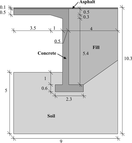
Assuming that the thickness of the bridge deck and abutment are equal, slender parts have been shown to cause larger temperature differences between the structural parts. Also, a thin asphalt layer leads to larger temperature differences.⁴ Based on this information, a relatively small bridge geometry was chosen for this study ( Fig. 1). The model thus corresponds to a realistic yet unfavorable bridge geometry, regarding temperature differences between structural parts. The height of the bridge corresponds to the minimum height of 4.7 m required in Sweden for road traffic under the bridge.

The material parameters used are listed in Table 1. For concrete and asphalt, the chosen values correspond to the mean of values given by the respective reference in Table 1, except for absorptivity and emissivity, for which the higher values were chosen. These values are assumed to correspond to newly placed asphalt, and choosing the higher values will increase the temperature difference between the bridge deck and abutment. The parameter values used for soil and fill were, on the other hand, chosen directly for two different soil types.⁹ Water-saturated clay was chosen for the soil, and a dry gravel with a porosity of 0.4 was chosen for the fill. The clay was chosen owing to its high density, heat conductivity and specific heat capacity, leading to a larger influence on the temperature in the structure, which had been shown to increase the temperature difference between the parts. Since the fill is covered from above by the asphalt paving on the road, and since capillary forces can be neglected in friction soils, the gravel chosen as fill was assumed to be dry, which reduces its density, heat conductivity and specific heat capacity.

Table 1: Parameter values used in the simulations

Material	Parameter	Unit	Value used	Min. value	Max. value	Ref.
Concrete	Density	kg/m^3	2350	2300	2400	[10]
	Heat conductivity	W/(m·°C)	2.05	1.60	2.50
	Specific heat capacity	J/(kg·°C)	900	800	1000
Asphalt	Density	kg/m^3	2170	2100	2240	[11]
	Heat conductivity	W/(m·°C)	1.6	0.7	2.5
	Specific heat capacity	J/(kg·°C)	880	840	920
	Emissivity		0.95	0.85	0.95
	Absorptivity		0.95	0.80	0.95	[12]
Soil (wet clay)	Density	kg/m^3	2000			[9]
	Heat conductivity	W/(m·°C)	1.0
	Specific heat capacity	J/(kg·°C)	1600
Fill (dry gravel)	Density	kg/m^3	1688			[9]
	Heat conductivity	W/(m·°C)	0.45
	Specific heat capacity	J/(kg·°C)	845

Simulations were performed using four-node rectangular heat transfer elements, with exceptions in areas close to the non-right angles of the model, where three-node triangular elements were also used. The elements were of the size 0.05 × 0.05 m² in the bridge structure and asphalt layer, and were gradually increased to 0.25 × 0.25 m² in the soil and gravel.

It has previously been found that the temperature difference between the structural parts produced by the model has an uncertainty of up to 1.5°C at a given point in time, but that this uncertainty is negligible in a long-term perspective.⁵ For this reason, 1.5°C should be added to short-term temperature differences produced by the model, e.g. characteristic values, while this model uncertainty is disregarded in long-term perspectives, e.g. for quasi-permanent values.

Long-Term Data Series

The data used in this study were obtained from the Swedish Metrological and Hydrological Institute (SMHI), and consisted of hourly values for air temperature, wind speed, solar radiation and long-wave radiation, for time periods of at least 10 years. The data series are listed in Table 2 and the locations from which the data are taken are shown in Fig. 2. The data are available for download from the website of the institute.

Fig. 2: Map of Sweden with the marked locations from which the weather data used in the study are taken

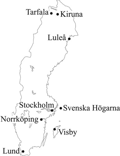
Table 2: List of data series used in the simulations

Location	Data period	No. of years
Tarfala	2008–2017	10
Kiruna	2008–2017	10
Luleå	1988–1997	10
Svenska Högarna	2008–2017	10
Stockholm	1986–1997	12
Norrköping	2008–2017	10
Visby	2008–2017	10
Lund	1983–1999	16

Three of the locations are in the northern part of the country, of which one (Luleå) is situated by the coast of the Gulf of Bothnia. Of the other two, the weather station in Kiruna is situated at 460 m altitude, and the other (Tarfala) is situated in a valley in the Scandinavian mountains, at an altitude of 1150 m. Of the five southern locations, two are in strongly maritime environments. These are Visby, situated on the island of Gotland in the Baltic Sea, and Svenska Högarna, situated on one of the outermost islands of the Stockholm archipelago. The other three southern locations, Stockholm, Norrköping and Lund, are not far from the open sea, but less influenced by it than the other two.

Model Definitions and Initial Results

An example of the temperature distribution in the structural model is given in Fig. 3. The result shown is taken from the simulation of temperature using weather data from Lund, on 8 July 1991 at 7 pm, a time when the temperature difference between the bridge deck and abutment was unusually large. This occurred after a warm day (temperatures up to 30°C) with clear skies. It can be seen in Fig. 3 that the temperature in the structure changes in the lower part of the abutment, and also in the corner region. There are also temperature gradients present over both the bridge deck and abutment cross-section, but as the objective is to investigate temperature differences between structural parts, these gradients are not considered as influential.

Fig. 3: Temperature distribution in the structural model on 8 July 1991 at 7 pm, using data from Lund

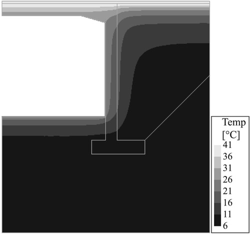
Apart from the gradients, the temperature is relatively constant in the structure, except for the corner area and the lower part of the abutment. Based on this observation, it was determined that the load case would assign constant temperatures to the major parts of the structural elements, and transition zones between these parts. The temperature in the load case is meant to vary linearly along the transition zones, in order for the load case to capture the gradual temperature change occurring in the corner and in the lower part of the abutment. As the load case is to be used in the design, it assigns temperature values to the entire structural model, and not just over the transition zones, for example, in order to cause correct restraining effects in the structure.

Figure 4 shows the division of the cross-section into parts with uniform temperature and transition zones. The temperature in the structural parts was calculated as the mean temperatures of the nodes belonging to the specific part in Fig. 4, and the difference in temperature was thus assumed to occur over the respective transition zones. Temperature differences between adjacent structural parts can thus occur between the bridge deck and the abutment, and between the abutment and the foundation. As tensile stresses in the transverse direction due to thermal actions occur in the colder structural part, and as either part can be colder than the other in both cases, four load cases were defined, as listed in Table 3.

Fig. 4: Definition of structural parts used in the study for temperature calculation. The mean temperatures of the darker grey areas are calculated and compared. The difference in temperature between these areas constitutes the load values

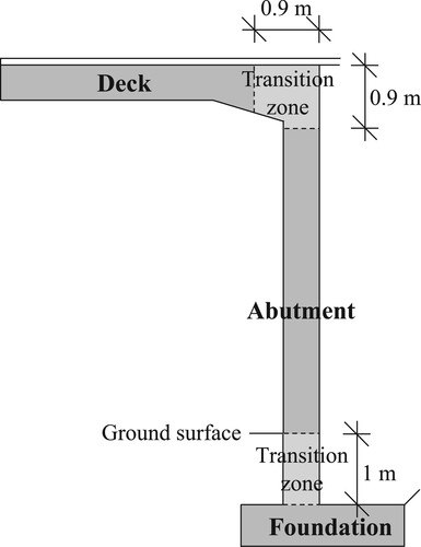
Table 3: Definition of the four load cases investigated, with the structural parts defined in Fig. 4*

Load case	Description
Positive temperature difference, deck–abutment	Deck warmer than abutment
Negative temperature difference, deck–abutment	Deck colder than abutment
Positive temperature difference, abutment–foundation	Abutment warmer than foundation
Negative temperature difference, abutment–foundation	Abutment colder than foundation

*The thermal actions listed will cause transverse tensile stresses in the colder structural part.

Using the definition of structural parts and transition zones shown in Fig. 4, the temperature differences between the parts were determined for each load step in the FE simulations. The three largest temperature differences for each load case are listed in Table 4. In Fig. 5, the temperature along the system line is shown for these occasions. The letters along the horizontal axis of Fig. 5 indicate some locations of interest along the system line, which are illustrated in the top part of the figure.

Fig. 5: Temperature variation along the system line, on the occasions of each of the largest temperature differences given in Table 4

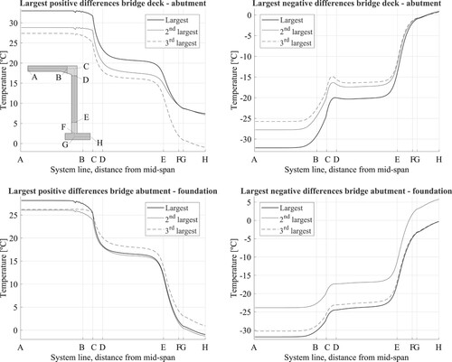
Table 4: The three largest temperature differences for each load case during the simulations

Load case	Largest temperature difference	2nd largest	3rd largest
Positive temperature difference, deck–abutment	13.0°C Lund, 8 July 1991	12.4°C Lund, 6 July 1985	12.3°C Kiruna, 11 June 2011
Negative temperature difference, deck–abutment	−12.3°C Kiruna, 8 January 2016	−10.8°C Kiruna, 6 January 2016	−9.7°C Kiruna, 6 January 2017
Positive temperature difference, abutment–foundation	16.7°C Kiruna, 11 June 2011	16.5°C Kiruna, 31 May 2013	16.1°C Kiruna, 10 July 2015
Negative temperature difference, abutment–foundation	−21.2°C Kiruna, 6 February 2012	−20.5°C Stockholm, 11 January 1987	−20.2°C Kiruna, 5 January 2012

Figure 5 reveals that the temperature changes between the bridge deck and abutment occur within the transition zone in the top of the abutment (between C and D) when the deck is warmer, and in the entire transition zone (between B and D) when the bridge deck is colder. In the abutment–foundation area, the largest change occurs in the bottom part of the abutment, within the transition zone between E and F. The chosen division into structural parts therefore seems reasonable.

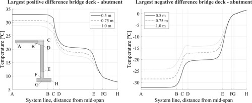
Investigations into the effect of changing the geometry showed that the thickness of the structural parts had a negligible influence on the length of the transition zones, as exemplified in Fig. 6. The figure shows the temperature along the system line at the time for the largest positive and negative temperature difference between the bridge deck and abutment, for three different cross-sectional thicknesses of the bridge deck and abutment. The figure thus shows that the transition zones are valid for thicknesses in the range 0.5–1.0 m.

Fig. 6: Temperature along the system line for analyses with different thicknesses on deck and abutment

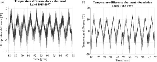
Figure 7 shows the temperature difference between the structural parts as defined in Fig. 4 for the entire simulation period from Luleå, 1988–1997. Figure 7 clearly illustrates the seasonal variations in the temperature difference, with the bridge deck being warmer than the abutment in summer, as well as the abutment being warmer than the foundation. During winter, the situation is the opposite, with the foundation being the warmest part, followed by the abutment, while the bridge deck generally is the coldest. The load cases listed in Table 3 are thereby active at different times; generally speaking, the first and third load cases are active during the summer and the second and fourth during the winter.

Fig. 7: Temperature difference between (a) bridge deck and abutment and (b) abutment and foundation, using weather data from Luleå from the period 1988–1997

Characteristic Load Values

To determine characteristic load values for the four load cases defined in Table 3, the generalized extreme value (GEV) distribution was used.¹³ The extreme values to be used as the variable in the GEV distribution are found by dividing the temperature difference over time, illustrated in Fig. 7, into reference periods, and choosing the highest (or lowest) value of each period for the GEV analysis. The choice of the length of the reference periods is thereby of importance to the result, and should be made in such a way that the extreme values in adjacent reference periods are statistically independent of each other. The ideal reference period is thereby 1 year in this application, as the temperature difference was shown in Fig. 7 to have a seasonal variation.

However, the fitting of a GEV distribution curve can be difficult if there are too few extreme values. For this reason, in addition to the 1 year reference period, calculations with 3 day seasonal periods were also made, meaning that the data were divided into 3 day periods, and only periods within April–September were considered for positive temperature differences, while periods within October–March were considered for negative differences. Three-day seasonal reference periods have previously been used for determination of temperature gradients in the Eurocode,⁴ thus showing that this is a reasonable assumption. Each set of extreme values was plotted as a cumulative distribution function (cdf), and the GEV distribution was then fitted to the values using the MATLAB^® function gevfit. The type III extreme value distribution (Weibull) was chosen by the function as the best curve fit in all cases.

Figure 8 shows the results of a comparison between using 1 year and 3 day seasonal reference periods, when using the weather data from Luleå and investigating positive temperature differences between deck and abutment. Figure 8 illustrates the uncertainty of using too few reference periods, and also shows that the 3 day seasonal reference period gives a good fit to the extreme value distribution.

Fig. 8: Cumulative distribution functions of the extreme values obtained using the weather data from Luleå and load case-positive temperature difference between deck and abutment. Results using both 3 day seasonal and 1 year reference periods are shown. GEV = generalized extreme value

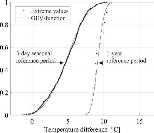
The GEV distributions can then be used to estimate the characteristic load values, by reading the load value that is exceeded every 50 years according to Fig. 8. If a 1 year reference period is used, the 50 year value corresponds to the 1 – 1/50 = 0.98 percentile. For 3 day seasonal reference periods, there are 61 reference periods per year, and the 50 year load value corresponds to the 1 – 1/(50 × 61) = 0.99967 percentile. The resulting characteristic load values for the respective data series and load cases, determined using 3 day seasonal reference periods, are displayed in Table 5. To account for the model uncertainty, which was estimated to be 1.5°C,⁵ this value has been added to the values obtained in the study.

Table 5: Characteristic temperature differences determined for the different data series using 3 day seasonal reference periods, and for the four load cases defined in Table 3*

Data series	Characteristic temperature difference (°C), deck–abutment		Characteristic temperature difference (°C), abutment–foundation
	Positive	Negative	Positive	Negative
Tarfala 2008–2017	13.5	−9.7	15.1	−16.7
Kiruna 2008–2017	14.0	−13.7	18.5	−25.0
Luleå 1988–1997	12.0	−12.0	17.3	−26.7
Svenska Högarna 2008–2017	11.4	−6.1	14.6	−15.8
Stockholm 1986–1997	13.0	−10.5	16.8	−21.7
Norrköping 2008–2017	14.1	−11.2	15.4	−21.8
Visby 2008–2017	11.8	−7.5	15.4	−17.5
Lund 1984–1999	14.7	−9.5	14.9	−17.5

*The uncertainty of the model, estimated to be 1.5°C, has been added to the given values.

The largest value of each load case is given in bold.

It can be seen in Table 5 that the temperature difference is larger between abutment and foundation than between deck and abutment. The largest values are found for negative temperature differences between abutment and foundation. This was also the load case that showed the largest spread in the results from the different locations. It can also be seen that the load values are relatively low in the maritime locations of Svenska Högarna and Visby, while they are relatively high in the inland location of Kiruna. An important climatic difference between maritime and inland locations is the air temperature fluctuations, which generally are smaller in coastal areas. Therefore, the difference in load values found between the locations is expected to be related to the variations in air temperature over the year.

To find a possible correlation between the load values and air temperature variations, the results in Table 5 were compared with air temperature data from the different locations. As the temperature in the foundation changes very slowly over the year,⁵ the characteristic temperature difference between abutment and foundation was expected to depend on the seasonal temperature variations. For this reason, the abutment–foundation thermal load values were compared with the difference in mean temperature between January and July. The temperature in the abutment and especially the deck, on the other hand, adjusts more rapidly to the air temperature, and the difference in characteristic value is therefore more dependent on the magnitude of rapid temperature changes. Therefore, the average differences between the maximum and minimum temperature in January and in July, respectively, were used in these comparisons. Weather data from January were used for the negative values and data from July for the positive, as the load values have been shown to be positive in summer and negative in winter ( Fig. 7). The resulting graphs are presented in Fig. 9.

Fig. 9: Characteristic thermal load values from Table 5 plotted against different variations in air temperature. For three of the cases, a correlation is possible

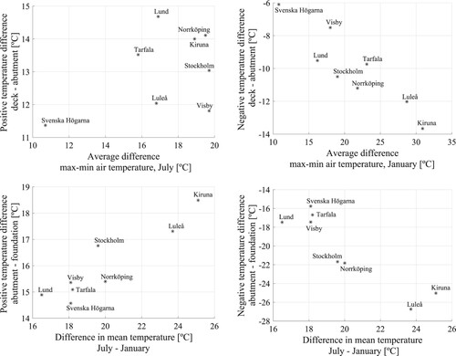
Figure 9 shows that in all cases except for the positive temperature difference between deck and abutment, it is realistic to assume a correlation between the load case value and the air temperature data. This can be used to determine in which locations the load value will be largest, within other geographic areas, or to estimate the actual load value. However, as other parameters also affect the result, estimations of load values using this methodology would include large uncertainties. For the load case where a correlation is not likely, i.e. positive temperature differences between deck and abutment, other parameters such as the solar radiation could be affecting the result too much for the temperature to be used as a guiding tool. Alternatively, the maximum and minimum monthly temperatures are not representative of the air temperature variations that occur.

The same trends as in Table 5 can be seen in Fig. 9 regarding the effect of the surrounding climate. The maritime location Svenska Högarna has the lowest temperature difference between parts, which can be connected to a lower difference in both mean temperature between July and January and between the maximum and minimum air temperatures within those months. The northern inland location of Kiruna, in contrast, has large differences, both regarding the structural temperatures and in the surrounding air. This shows that there is a connection between the surrounding climate and the differences in temperature between structural parts, which can be valuable for other locations with similar climates to the studied locations.

Quasi-Permanent Load Value

In the Eurocode,¹⁴ the quasi-permanent load value is defined as a value where “the total period of time for which it will be exceeded is a large fraction of the reference period”. It is also stated in the same document that for loads on building floors, the median value is often used, and that the mean value during a chosen period of time can alternatively be used. No information is given regarding thermal loads.

In the case of temperature differences between deck and abutment in portal frame bridges, the bridge deck is shown to be warmer than the abutment more than half of the time, meaning that the median load value would be positive. As the thermal load cases have been divided into two parts, one for positive values and one for negative values, using the median value only produces a load value for one of the two cases, and no load value would be obtained for the case with negative temperature differences between deck and abutment. As this would risk underestimating the “quasi-permanent” load effect, the load case in this study is instead defined as follows: The median value during the time that the load is active, but only during the half of the year when the load is dominating. This means that positive temperature differences are only considered during April to September, and negative differences during October to March.

Considering only the time when the load is active means that only positive load values are considered when determining the positive quasi-permanent load value, and only negative values are considered when determining the negative load value. Only considering the values during the half of the year when the load is dominating increases the load values slightly, as the load is generally small when it occurs during the rest of the year. In addition, the load generally has a short duration in such cases, which is not likely to cause any significant long-term effects on the structure.

Using this definition of the quasi-permanent load values, the values can be calculated for each data set, with the results shown in Table 6. As the comparison of measured and simulated temperature did not show any significant difference between the temperature difference between deck and abutment over time in the verification of the simulation model,⁵ no adjustment is needed to account for the model uncertainty.

Table 6: Quasi-permanent load values*

Data series	Quasi-permanent temperature difference, deck–abutment		Quasi-permanent temperature difference, abutment–foundation
	Positive value (°C)	Negative value (°C)	Positive value (°C)	Negative value (°C)
Tarfala 2008–2017	3.46	−1.43	5.01	−4.06
Kiruna 2008–2017	3.34	−1.77	6.06	−5.18
Luleå 1983–1997	3.42	−1.83	6.54	−4.64
Svenska Högarna 2008–2017	2.67	−0.80	4.79	−3.80
Stockholm 1983–1997	3.33	−1.26	5.85	−3.79
Norrköping 2008–2017	3.99	−1.14	5.07	−4.29
Visby 2008–2017	3.08	−0.82	4.86	−3.87
Lund 1984–1999	3.41	−1.04	5.31	−3.30

*Calculated as median values for times when the load is present during the half of the year when the load is occurring frequently.

The largest value of each load case is given in bold.

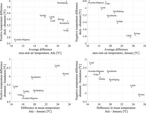
Table 6 shows that the load values are larger for the abutment–foundation connection than for the deck–abutment connection. In addition, the largest values for abutment–foundation for both positive and negative differences are found using data from Luleå and Kiruna, as was the case for the characteristic load. A possible correlation between the load values and the same air temperature variations as used in Fig. 9 was also made, resulting in the graphs presented in Fig. 10. Figure 10 shows that possible correlations are found for the same three cases as for the characteristic load.

Fig. 10: Quasi-permanent thermal load values from Table 6 plotted against different variations in air temperature. For three of the cases, a correlation is possible

Discussion

The results obtained in this study could be used in the determination of new load values, which may, for example, consist of one characteristic and one quasi-permanent load value for each of the four load types, combined with a linear temperature transition along the system line in the frame corner and in the bottom of the abutment. This would lead to a more detailed and accurate load case than the one presented in the Eurocode.¹

The analyses of temperature variation along the system line showed consistent results with transition zones in the bottom of the abutment and in the corner area, as shown in Fig. 5. It was also shown that the transition zones are not dependent on the cross-sectional thickness, when varied within 0.5–1.0 m. The results shown are, however, based on the temperature distribution on only a few occasions. However, the occasions chosen represent the largest temperature differences between the parts, and it seems reasonable to analyze the temperature distribution at times when the temperature differences are large and distinct.

As this study was performed using weather data from different parts of Sweden, the largest load values can probably be used in designs within the entire country. A relationship between variations in air temperature and the obtained load values was found in three of the four load cases. Therefore, a simpler investigation into air temperature can be performed and compared with the results presented, to estimate the likeliness of the chosen location having a worse climate than the locations used in this study. The relationship can be used to determine the locations in which the largest load values can be expected within other geographic areas, or to estimate the actual load values. It should, however, be noted that the air temperature data presented in Figs. 9 and 10 are based on the data used in the simulations. To compare the air temperature data with other locations, the data should preferably have been measured with the same interval, and during the same period. This comparison could probably be made for locations outside Sweden with similar climates, but may be more unreliable in locations where the climate is significantly different, as, for instance, solar radiation can have a larger impact and seasonal temperature variations are profoundly different in locations at other latitudes. However, owing to the limited studies that have been performed previously,² the present study still adds significantly to the available data on the topic.

The definition of quasi-permanent load values used in this study can also be discussed. The quasi-permanent load in bridge design is used for crack width limitation, which, in turn, is related to the risk of corrosion. Because of this, the definition chosen should correspond to a method relevant to corrosion development in cracked structures. The way in which the magnitude of corrosion depends on the crack width and exposure time is, however, not very clear, and although studies have shown that wide cracks cause corrosion to develop more rapidly initially, there is some controversy over whether this also holds true for long-term effects.^15,16 It can therefore be debated whether the median crack width over half the year is the best way to define a load aiming to limit corrosion, but the approach may be regarded as conservative, as the smaller crack widths during the other half of the year are disregarded in the analysis.

Conclusions

This paper investigates the temperature in portal frame bridges, using simulations with weather data from several Swedish locations, with a focus on temperature differences between structural parts. Four different load cases are defined, describing temperature differences between bridge deck and abutment, and between abutment and foundation. Characteristic values were calculated for each load case and location, and were smaller than the present 15°C value for differences between deck and abutment, but larger for differences between abutment and foundation. The quasi-permanent values were, however, significantly lower than the 15°C, with a maximum value for all data series, load cases and load definitions of 6.5°C, i.e. less than half of the present value. Furthermore, the description of temperature variation along the system line shows that the temperature change is gradual. The results can be used in the consideration of new and more detailed descriptions of the temperature difference between structural parts of portal frame bridges. This will, in turn, lead to lower stress values resulting from the calculations.

Additional information

Funding

This research was sponsored by the Swedish Transport Administration [grant number 2013-016] and Svenska Byggbranschens Utvecklingsfond (SBUF), the Swedish construction industrýs organization for research and development [grant number 13136].

References

- CEN (European Committee for Standardization). EN 1991-1-5: Actions on structures: General actions - Thermal actions. Brussels, 2003.
- CEN (European Committee for Standardization). Background document to ENV 1991-2-5: Thermal actions, Draft: February, Brussels, 1996.
- Vägverket. Vägverkets allmänna tekniska beskrivning för nybyggande och förbättring av broar, Bro 2004 [The Swedish Road Administration’s general technical description for construction and improvement of bridges, Bridge 2004]. Publication 2004:56, ISSN 1401-9612.
- Gottsäter E, Larsson Ivanov O, Molnár M, Crocetti R, Nilenius F, Plos M. Simulation of thermal load distribution in portal frame bridges. Eng. Struct. 2017; 143: 219–231. doi: 10.1016/j.engstruct.2017.04.012
- Gottsäter E, Larsson Ivanov O, Molnár M, Plos M. Validation of temperature simulations in a portal frame bridge. Structures. 2018; 15: 341–348. doi: 10.1016/j.istruc.2018.07.007
- Trafikverket. TRVR Bro 11. 2011. ISBN: 978-91-7467-154-4.
- Gottsäter E, Larsson Ivanov O, Crocetti R, Molnár M, Plos M. Comparison of models for design of portal frame bridges with regard to restraint forces. ASCE structures congress 2017. Denver: American Society of Civil Engineers, 2017.
- Larsson O. Modelling of temperature profiles in a concrete slab under climatic exposure. Struct. Concr. 2009; 10: 193–201. doi: 10.1680/stco.2009.10.4.193
- Sundberg J. 1991. Termiska egenskaper i jord och berg [Thermal Properties in Soil and Rock]. Statens Geotekniska Institut: Linköping, 1991.
- Ljungkrantz C, Möller G, Petersons N. 1994. Betonghandbok – material [Concrete handbook - material]. Svensk byggtjänst: Stockholm, 1994.
- Larsson O. Climate related thermal actions for reliable design of concrete structures. Division of Structural Engineering, Lund University, 2012.
- Bretz S, Akbari H, Rosenfeld A. Practical issues for using solar-reflective materials to mitigate urban heat islands. Atmos. Environ. 1997; 32, 95–101. doi: 10.1016/S1352-2310(97)00182-9
- Coles S. An Introduction to Statistical Modeling of Extreme Values. Springer: London, 2004.
- CEN (European Committee for Standardization). EN 1990: Basis of structural design, Brussels, 2002.
- Otieno MB, Alexander MG, Beushausen HD. Corrosion in cracked and uncracked concrete – influence of crack width, concrete quality and crack reopening. Mag. Concr. Res. 2010; 62: 393–404. doi: 10.1680/macr.2010.62.6.393
- François R, Khan I, Vu NA, Mercado H, Castel A. Study of the impact of localised cracks on the corrosion mechanism. Eur. J. Environ. Civil Eng. 2012; 16: 392–401. doi: 10.1080/19648189.2012.667982