IABSE Task Group 3.1 Benchmark Results. Numerical Full Bridge Stability and Buffeting Simulations

Abstract

Aerodynamic stability and buffeting response due to turbulent wind have a fundamental importance for long-span bridge design. However, there are no benchmark cases that can be used as a reference estimate for an independent validation of the numerical methods and theoretical approximations. Therefore, the IABSE Task Group 3.1 proposal is to fill this gap by defining a reasonably well predicted set case for the response to wind of long-span bridges, both in terms of aerodynamic stability and buffeting. Specifically, a statistical analysis was performed on the numerical results collected by the task group participants, who used their own methodology and tools (either in time domain and/or frequency domain) to predict the bridge stability to flutter and buffeting response to wind, sharing the same input data (wind conditions, bridge structural properties, and deck aerodynamic coefficients). The benchmark results presented in this paper can be used as a point of reference for other numerical codes, and they include the onset of flutter speed, damping ratio variation with mean wind speed and the root mean square of the displacements as a function of mean wind speed, power spectral density values, and time histories of displacements.

Keywords:

• benchmark
• aeroelasticity
• flutter
• buffeting
• long-span bridge
• validation
• simulation

Introduction

Numerical tools are fundamental in the design of long-span bridges. Stability, comfort, fatigue and structural strength of long-span bridges are indeed quantified through numerical simulations of the expected behaviour of the structure, using approaches based on aerodynamic coefficients measured in wind tunnels and by structural Finite Element Method (FEM) numerical models. Different theoretical approximations and numerical models have been developed during the last 60 years to simulate the response of bridges to turbulent wind. The aerodynamics of the bridge deck is the predominant element in the bridge response to wind.^1–3 The theoretical approximations are based on extensions to the quasi-steady theory through the application of aerodynamic coefficients (steady-state coefficients and motional aerodynamic derivatives also known as flutter derivatives). The numerical application of this theory may vary to a great extent since deck flutter derivatives vary depending on reduced velocity, mean angle of attack and amplitude of motion, subject to various theoretical interpretations. Aerodynamic nonlinearity may also be taken into account, which adds further complexity to the problem. However, this is beyond the scope of this article.

Approaches working in the frequency domain^4–8 are widely used where the dynamic responses to turbulent winds are predicted based on wind velocity reference spectra, with key parameters being mean wind speed, turbulence intensity and spatial correlation. The numerical models developed in the time domain^9,10 have greater complexity in implementing the reduced velocity dependency of the aerodynamic forces but have the advantage being able to consider transient contributions and time-varying wind scenarios,^11,12 with the possibility of also reproducing the aerodynamic^13–22 and structural nonlinearities. Bridge response near flutter instability or transient wind gusts cannot be simulated through frequency domain approaches because the transient response of the system is neglected. For this reason, the peak values of the bridge aeroelastic response cannot be well reproduced for wind speeds approaching instability.

Peak values cannot be estimated directly by frequency domain simulations, which rely on results from statistical signal analysis. Time domain approaches are able to input directly the response time histories required for full statistical estimations including peak values, with a heavier requirement in the reproduction of a given wind scenario that has to be described through the repetition of the numerical simulations using a sufficient number of possible wind velocity time histories. The aerodynamic stability is usually evaluated by solving the generalized state equation comprising mass, damping and stiffness matrices developed in the frequency domain or in the time domain approaches including the equivalent effects of the aerodynamic forces through a linearized approach.

Both frequency domain approaches and time domain approaches are commonly used by the industrial and research groups that are internationally involved in bridge design, where almost everyone adopts their own originally developed methodology and tools. Owing to the variety of implementation, it is not uncommon for the interpretation and comparison of results to be difficult at times. For this reason, the authors of this article decided to join in the IABSE Task Group 3.1 (extended name: “Super-Long-Span Bridge Aerodynamics”) to investigate the level of uncertainty and comparability of the results produced by their various theoretical interpretations and numerical simulations. It should be noted that the comparisons in this article are restricted to the implementation of similar theoretical approximations and not directly to results obtained either experimentally or from full-scale observation.

The aim of the task group is to design a validation procedure for numerical models that simulate the aeroelastic response of a full bridge. The reference values provided by the benchmark were achieved by analysing the output of state-of-the-art numerical procedures.

The Task Group (TG) decided to set up a benchmark procedure that consists of multiple steps with an increasing level of complexity. A detailed description of the benchmark structure and the results of previous steps can be found in Ref. [12]. For each step the same input data were used and shared among all the participants, and the results obtained through different methodologies were analysed to define reference values giving a baseline for the validation of theoretical methods and numerical procedures.

TG members were asked to use their own consolidated methodology to simulate bridge behaviour starting from input data provided in a format typical of bridge aeroelasticity applications: geometry, modal data for the structural dynamics (modal mass, frequency, damping, mode shape), wind field characteristics, aerodynamic static coefficients and flutter derivatives defined for different wind angles of attack and speed range.

It was expected that the frequency domain approaches would result in similar prediction performances while more differences were expected from the time domain methods. For time domain simulations, several ways to reproduce the aerodynamic force dependency on wind velocity and angle of attack are proposed in the literature: convolution integral, band superposition, rheologic models, Volterra methods, Gaussian processes, and others.^{14,15,17–21,23,24}

While time domain methods are often used in literature to study nonlinearities of aerodynamic forces due to large variation of the wind angle of attack induced by turbulence and large deck rotations, the framework of the TG3.1 benchmark only considers the linear approaches, which are generally adopted by bridge designers since their mathematical model complexity²⁵ is deemed sufficient in practice. The only nonlinear effects considered in this benchmark are the static variation of the bridge deck rotation due to the mean wind loading, and the dependence on the reduced velocity of the aeroelastic coefficients.

The goal of TG3.1 is not to examine the details of the different methodologies and implementations, which are reported in Refs. [4,5,14,21,26–47], but rather to provide aerodynamic response predictions that can be used to define a benchmark, the assumption being that all the implemented methods have been calibrated against other methods and experiments, being widely used and applied to many different cases, hence all the results could be considered reliable and able to provide values with low dispersion, taking also into account that the benchmark participants are recognized experts in the field.

For full-bridge response analysis, a closed form solution cannot be formulated and therefore this working group believes that a sufficiently robust benchmark can only be inferred from the comparison of the available results. Relying on and the number of TG3.1 participants and their qualifications, it is assumed that the state-of-the-art is properly represented for the proposed activities and that the results presented depict what is nowadays achievable by the current state of knowledge.

The output of the work of TG3.1 is published for everyone who seeks a benchmark for comparison and validation of their future methodologies and numerical codes.

In this article, the Storebælt East Bridge in Denmark has been selected as representative of a typical long-span bridge.⁴⁸ The structural dynamics is defined through a modal approach using the first 12 eigenmodes obtained by finite element analysis during design of the bridge to form the bridge numerical model.⁴⁹ Aerodynamic and aeroelastic forces acting on the deck alone are considered, neglecting the wind and dynamic action of the towers, the main cable and hangers.

Compared to the previous steps of this study,^1,2 where only the deck cross section was considered, the present activity introduces additional complexity as the wind and the corresponding aerodynamic force correlation along the bridge are to be reproduced and the complete dynamic response of the bridge has to be taken into account.

Stability and buffeting are computed for two conditions: “Step A” of the benchmark assumes no static deformation of the bridge due to the average wind. “Step B” includes nonlinear static deformation of the bridge.

A set of aerodynamic static coefficients and flutter derivatives (Scanlan derivatives) was adopted from a similar single box bridge deck. They represent, compared to the information available for the Storebælt East Bridge, a more recent and complete data set in terms of reduced velocity range and mean angles of attack.

For consistency, the analytical Davenport aerodynamic admittance function² is used to define aerodynamic buffeting forces, considering both the along wind $u$ and vertical $w$ components of turbulence.

The input data provided to all TG 3.1 contributors are described in Section 2 and can be downloaded from the online supplemental data. The output results used in the benchmark are described and compared in Section 3. The base parameters defining the current study problem are given below, while the full set of input data and the study results are provided in the online supplemental data.

Stability and Buffeting Analysis

Steps A and B

As stated above, the analysis in this article is divided into two steps, called A and B, as follows.

1. Step A does not consider the static deflection of the bridge, and flutter derivatives and admittance functions are taken at zero-degree angle of attack for all the deck sections.

2. Step B, instead, considers the dependence of the aerodynamic derivatives upon the nonlinear static deck rotation.

In this article, the input data for the benchmark are reported as follows: structural data in Section 2.2, and incoming turbulent wind and aerodynamic forces in Sections 2.3 and 2.4, respectively.

Structural Data

The bridge is modelled by applying the modal approach considering the first 12 eigenmodes of vibration obtained by an eigenvalue–eigenvector analysis. Natural frequencies, generalized masses and modal damping are reported in Table 1.

Table 1: Modal parameters

No.	Mode	Frequency (Hz)	Generalized modal mass (kg)	Damping ratio, ξ (%)
1	Horizontal 1	0.0521	1.7424 e + 07	0.3
2	Vertical 1	0.0839	1.8231 e + 07	0.3
3	Vertical 2	0.0998	1.6682 e + 07	0.3
4	Horizontal 2	0.1179	1.8981 e + 07	0.3
5	Vertical 3	0.1317	1.2559 e + 07	0.3
6	Vertical 4	0.1345	2.1215 e + 07	0.3
7	Vertical 5	0.1827	1.7402 e + 07	0.3
8	Horizontal 3	0.1866	2.4313 e + 07	0.3
9	Torsional 1	0.2784	1.6827e + 09	0.3
10	Vertical 6	0.2815	1.6538 e + 07	0.3
11	Torsional 2	0.3833	1.9232e + 09	0.3
12	Vertical 7	0.3975	1.7269e + 07	0.3

The considered set of 12 modes includes the first two torsional modes, the first mode having the antinode at mid-span and the second mode with a node at mid-span. Seven vertical modes and three lateral modes are also included. These mode shapes were used by all participants. As an example, Fig. 1 shows the first and second vertical and torsional modes.

Fig. 1: Lateral (in m), vertical (in m), and torsional (in degrees) components of selected modal shapes

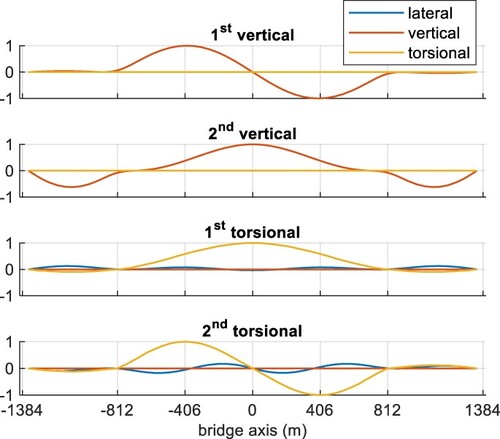
The modal approach with 12 modes was used to compute the dynamic response to the wind turbulence (buffeting). The same modal basis was also used to find an approximate static deflection induced by the mean wind loading, considering the nonlinear dependence upon the mean angle of attack.

Incoming Turbulent Wind

The mean wind speed $U$, and the along-wind and the vertical components ($u$ and $w$) of the wind turbulence are considered in the simulations.

Four mean wind speed scenarios are considered to compare results with an increasing level of aerodynamic coupling up to a wind speed close to the flutter instability. Table 2 reports power spectral densities as a function of the frequency $f$ and other parameters of turbulence. The cross-power spectrum $S_{\mathrm{uw}}\left(f\right)$ of the incoming turbulence has been set to zero, since it does not strongly affect the response of the bridge.⁵⁰ Additionally, the spatial coherence of u or w at two different points P and Q is defined as (1) ${\mathrm{\Lambda }}_{\mathrm{ii}}=\exp \left(-{\displaystyle \frac{2\sqrt{{\left(C_{\mathrm{ix}}\mathrm{\Delta }x\right)}^2+{\left(C_{\mathrm{iz}}\mathrm{\Delta }z\right)}^2}f}{U_P+U_Q}}\right)$(1) where $i=u$or $w$, $C_{\mathrm{ux}}=10$, $C_{\mathrm{uz}}=10$, $C_{\mathrm{wx}}=6.50$, $C_{\mathrm{wz}}=3$, $\mathrm{\Delta }z=z_P-z_Q$ and $\mathrm{\Delta }x=x_P-x_Q$.

Table 2: Incoming wind characteristics

Wind speeds	U = 15, 30, 45, 60 m/s
Air density	$\rho =1.22$ kg/m^3
Turbulence intensity	$I_u={\displaystyle \frac{{\sigma }_u}{U}=0.10}$; $I_w={\displaystyle \frac{{\sigma }_w}{U}=0.05}$
Integral length scale	${}^x{L}_u=200\mathrm{m}$; ${}^x{L}_w=20\mathrm{m}$
u and w spectra	${\displaystyle \frac{f\cdot S_u\left(f\right)}{{\sigma }_u^2}={\displaystyle \frac{4\left({\displaystyle \frac{f{}^x{L}_u}{U}}\right)}{{\left[1+70.8{\left({\displaystyle \frac{f{}^x{L}_u}{U}}\right)}^2\right]}^{5/6}}}}$${\displaystyle \frac{f\cdot S_w\left(f\right)}{{\sigma }_w^2}={\displaystyle \frac{4\left({\displaystyle \frac{f{}^x{L}_w}{U}}\right)\left(1+755.2{\left({\displaystyle \frac{f{}^x{L}_w}{U}}\right)}^2\right)}{{\left[1+283.2{\left({\displaystyle \frac{f{}^x{L}_w}{U}}\right)}^2\right]}^{11/6}}}}$
	$S_{\mathrm{uw}}\left(f\right)=0$

Moreover, for each mean wind speed, ten time histories of turbulent wind velocities were generated in the 90 sections reported with red lines in Fig. 2, using the same wind characteristics, to allow the application of the time domain approaches. Each time history is 10 minutes long with a sampling frequency of 20 Hz. For the 45 m/s case, longer time histories of 1 h duration are also provided to account for the low frequency contributions.

Fig. 2: Position of the 90 sections at deck level along the bridge axis (red lines)

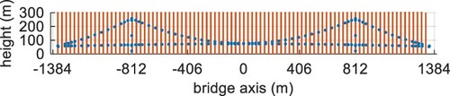
A harmonic superposition method is used for the generation of the time histories.^51–53 The method used for the wind generation was selected for convenience: the investigation of the wind field generation problem is not a task of the benchmark, and it is beyond the scope of this study. Ten time histories for each mean wind speed were generated every 30 m along the deck and were distributed to all the participants. These time histories are also available in the online supplemental data.

Aerodynamic Forces

The aerodynamic forces and moment are defined following the currently adopted theoretical models where the aerodynamic forces are a function of turbulence and of the deck motion and are defined by the static aerodynamic coefficients, the aerodynamic admittance function and the flutter derivatives identified around different static angles of attack of the deck. For simplicity, aerodynamic forces are considered only on the deck as mentioned previously.

In this benchmark, the aerodynamic data are taken from wind tunnel tests on the Yavuz Sultan Selim Bridge deck (Third Bosphorus Bridge) without windscreens.⁵⁴ The sign conventions for aerodynamic forces, deck displacements and wind velocity components are shown in Fig. 3.

Fig. 3: Sign conventions

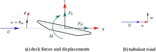
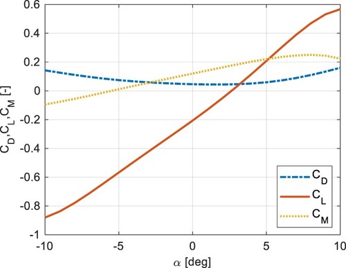
Figure 4 defines the steady drag, lift and moment coefficient per unit length as functions of the angle of attack$\alpha$: (2) ${\left\{\begin{array}{c}{F}_D\\ F_L\\ M\end{array}\right\}}_{\mathrm{ST}}={\displaystyle \frac{1}{2}\rho U^{2}B\left[\begin{array}{c}{C}_D\left(\alpha \right)\\ C_L\left(\alpha \right)\\ B{C}_M\left(\alpha \right)\end{array}\right]}$(2) where B is the deck chord ($B=31\mathrm{m}$), $U$ the mean wind velocity and $\rho$ is the air density. $C_D,C_L,C_M$ are, respectively, the drag, lift and moment static coefficients in wind coordinates.

Fig. 4: Static aerodynamic coefficients as a function of the angle of attack

The aeroelastic forces (motion-dependent or self-excited forces), $F_{\mathrm{se}}$, are here defined through the flutter derivatives reported below in the POLIMI formulation,⁵⁵ which has the advantage that flutter derivatives, defined in this way, converge to the quasi-steady theory (QST) values for reduced velocities $U^{\ast }=U/\mathrm{fB}$ greater than 10–15 (coefficients in the classical Scanlan formulation have also been distributed to participants): (3) $\begin{array}{rl}{D}_{\mathrm{se}}& ={\displaystyle \frac{1}{2}\rho U^{2}B}\\ & \left(\begin{array}{c}-p_1^{\ast }{\displaystyle \frac{\dot{z}}{U}-p_2^{\ast }{\displaystyle \frac{B\dot{\theta }}{U}+p_3^{\ast }\theta +\cdots }}\\ {\displaystyle \frac{2{\pi }^3}{U^{\ast }2}{p}_4^{\ast }{\displaystyle \frac{z}{B}-p_5^{\ast }{\displaystyle \frac{\dot{y}}{U}+{\displaystyle \frac{2{\pi }^3}{U^{\ast }2}{p}_6^{\ast }{\displaystyle \frac{y}{B}}}}}}\end{array}\right)\end{array}$(3) (4) $\begin{array}{rl}{L}_{\mathrm{se}}& ={\displaystyle \frac{1}{2}\rho U^{2}B}\\ & \left(\begin{array}{c}-h_1^{\ast }{\displaystyle \frac{\dot{z}}{U}-h_2^{\ast }{\displaystyle \frac{B\dot{\theta }}{U}+h_3^{\ast }\theta +\cdots }}\\ {\displaystyle \frac{2{\pi }^3}{U^{\ast }2}{h}_4^{\ast }{\displaystyle \frac{z}{B}-h_5^{\ast }{\displaystyle \frac{\dot{y}}{U}+{\displaystyle \frac{2{\pi }^3}{U^{\ast }2}{h}_6^{\ast }{\displaystyle \frac{y}{B}}}}}}\end{array}\right)\end{array}$(4) (5) $\begin{array}{rl}{M}_{\mathrm{se}}& ={\displaystyle \frac{1}{2}\rho U^2{B}^2}\\ & \left(\begin{array}{c}-a_1^{\ast }{\displaystyle \frac{\dot{z}}{U}-a_2^{\ast }{\displaystyle \frac{B\dot{\theta }}{U}+a_3^{\ast }\theta +\cdots }}\\ {\displaystyle \frac{2{\pi }^3}{U^{\ast }2}{a}_4^{\ast }{\displaystyle \frac{z}{B}-a_5^{\ast }{\displaystyle \frac{\dot{y}}{U}+{\displaystyle \frac{2{\pi }^3}{U^{\ast }2}{a}_6^{\ast }{\displaystyle \frac{y}{B}}}}}}\end{array}\right)\end{array}$(5) where $y,z,\theta$ and $\dot{y},\dot{z},\dot{\theta }$ are the lateral, vertical and torsional displacements, and velocities. The eight flutter derivatives coefficients ($a_1^{\ast },a_2^{\ast },a_3^{\ast },a_4^{\ast },h_1^{\ast },h_2^{\ast },h_3^{\ast },h_4^{\ast }$) are provided at five mean angles of attack: ±4°, ±2° and 0° in the reduced velocity range 1 < $U^{\ast }$ < 17, where $f$ is the motion frequency. These flutter derivatives are reported in Fig. 5. The flutter derivatives not measured in the wind tunnel test, $p_{1-6}^{\ast }$, $a_{5-6}^{\ast }$, $h_{5-6}^{\ast }$, are derived from quasi-steady aerodynamic theory (QST)^56,57 to complete the full set of aerodynamic coefficients. These flutter derivatives are reported in Table 3.

Fig. 5: Lift and moment flutter derivatives as a function of reduced velocity U*, for several mean angles of attack. The markers at U* = 20 indicate the quasi-steady values of the coefficients

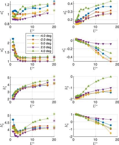
Table 3: Drag and lateral flutter derivative values based on QST, for several angles of attack

	$\alpha =-4^{\circ }$	$\alpha =-2^{\circ }$	$\alpha =0^{\circ }$	$\alpha =+2^{\circ }$	$\alpha =+4^{\circ }$
$a_5^{\ast }$	0.068	0.155	0.240	0.326	0.406
$a_6^{\ast }$	0.0	0.0	0.0	0.0	0.0
$h_5^{\ast }$	−0.989	−0.701	−0.412	−0.105	0.236
$h_6^{\ast }$	0.0	0.0	0.0	0.0	0.0
$p_1^{\ast }$	0.061	0.070	0.055	0.099	0.265
$p_2^{\ast }$	0.061	0.070	0.055	0.099	0.265
$p_3^{\ast }$	−0.434	−0.280	−0.151	0.047	0.383
$p_4^{\ast }$	0.0	0.0	0.0	0.0	0.0
$p_5^{\ast }$	0.132	0.108	0.093	0.088	0.102
$p_6^{\ast }$	0.0	0.0	0.0	0.0	0.0

These flutter derivatives have been extracted experimentally from rigid sectional models in a wind tunnel at a discrete number of reduced velocities requiring an interpolation and/or extrapolation to simulate conditions where experimental data are not available.⁵⁸ The same level of complexity is kept on purpose in the benchmark procedure, considering the data interpolation as part of the source of uncertainties.

The buffeting forces $F_{\mathrm{buff}}$per unit length due to incoming turbulent wind components $u$ and$w$ are defined in the frequency domain through aerodynamic admittance functions: (6) ${\left\{\begin{array}{c}\begin{array}{c}{\hat{F}}_D\\ {\hat{F}}_L\end{array}\\ \hat{M}\end{array}\right\}}_{\mathrm{buff}}={\displaystyle \frac{1}{2}\rho \mathrm{UB}\left[\begin{array}{cc}{\chi }_{\mathrm{Du}}^{\ast }& {\chi }_{\mathrm{Dw}}^{\ast }\\ {\chi }_{\mathrm{Lu}}^{\ast }& {\chi }_{\mathrm{Lw}}^{\ast }\\ B{\chi }_{\mathrm{Mu}}^{\ast }& B{\chi }_{\mathrm{Mw}}^{\ast }\end{array}\right]\left\{\begin{array}{c}\begin{array}{c}\hat{u}\left(f\right)\\ \hat{w}\left(f\right)\end{array}\end{array}\right\}}$(6) where the symbol $\stackrel{\stackrel{ˆ}{}}{}$ represents the Fourier transform, and ${\chi }^{\ast }$ are the aerodynamic admittance functions. The ${\chi }^{\ast }$functions depend on the mean angle of attack, and they are defined using the quasi-steady values weighted by the Davenport aerodynamic admittance function $A\left(U^{\ast }\right)$ as (7) $\begin{array}{c}\begin{array}{c}{\chi }_{\mathrm{Du}}^{\ast }=2C_{D}A\left(U^{\ast }\right)\\ {\chi }_{\mathrm{Lu}}^{\ast }=2C_{L}A\left(U^{\ast }\right)\\ {\chi }_{\mathrm{Mu}}^{\ast }=2C_{M}A\left(U^{\ast }\right)\end{array}\\ \begin{array}{c}{\chi }_{\mathrm{Dw}}^{\ast }=\left(K_D-C_L\right)A\left(U^{\ast }\right)\\ {\chi }_{\mathrm{Lw}}^{\ast }=\left(K_L+C_D\right)A\left(U^{\ast }\right)\\ {\chi }_{\mathrm{Mw}}^{\ast }=K_{M}A\left(U^{\ast }\right)\end{array}\end{array}$(7) where $K_D,$ $K_L$ and $K_M$ are the slopes of the static coefficients (in rad⁻¹), and $A\left(U^{\ast }\right)$ is a real function dependent on the reduced velocity (Davenport aerodynamic admittance): (8) $A\left(U^{\ast }\right)={\displaystyle \frac{2}{{\left({\displaystyle \frac{7}{U^{\ast }}}\right)}^2}\left({\displaystyle \frac{7}{U^{\ast }}-1+e^{-7/U^{\ast }}}\right)}$(8) Other admittance functions are available in the literature (e.g. Ref. [59]).

Benchmark Results

In this section, only a selected part of the study results is presented, while for those interested in comparing their own results in details, a complete set is provided in the online supplemental data.

In the analysis of the results, each contribution is defined anonymously by a number that is kept constant throughout the article. It should also be noted that there is no correspondence between the number assigned to each contribution and the order of the list of authors. For each benchmark result, a reference value, and a criterion for assessment/validation are given.

Aeroelastic Stability in Smooth Flow for Step A

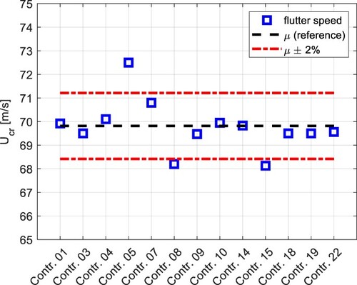
Figure 6 shows a plot of the flutter critical wind speeds predicted by different TG members for Step A, for a total of 13 contributions. In this case, the procedure to define a reference and acceptance criterion is as follows.

1. The mean ${\mu }^{\ast }$ and the standard deviation ${\sigma }^{\ast }$ of all data is computed (in this case, 13 values).

2. The values outside the range ${\mu }^{\ast }\pm {\sigma }^{\ast }$ are arbitrarily considered outlier data (in this case contribution 5, 8 and 15), and they are excluded for the definition of the reference value.

3. A reference mean value $\mu$ (69.8 m/s) is computed excluding the outlier data and taken as reference.

4. If the error between a contribution and the reference is less than ${ϵ}_{\mathrm{MAX}}=2\text{\%}$, the numerical procedure that produced the number is deemed to be sufficiently accurate (in this case ${ϵ}_{\mathrm{MAX}}=2\text{\%}$ is chosen arbitrarily by the TG).

Fig. 6: Flutter critical wind speed results from different programmes of the TG

For eight contributions in the frequency domain, Fig. 7 and Table 4 also show the trend of the total damping ratio (structural plus aerodynamic) as a function of the mean wind speed, for the mode that shows flutter instability (torsional branch). $\xi$ is defined as the ratio between the real part of the eigenvalue changed in sign and magnitude. Even though the spread of the flutter speed parameter is small, larger differences can be noted in some of the contributions.

Fig. 7: Total damping ratio of the unstable 1st torsional mode as a function of mean wind speed

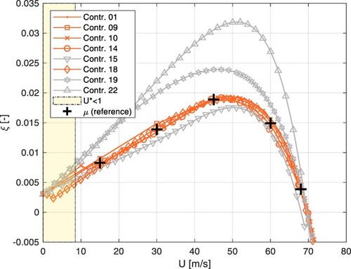
Table 4: Estimated values and spread of the total damping trend

		15 m/s	30 m/s	45 m/s	60 m/s	68 m/s
ξ	Μ	0.008	0.014	0.019	0.015	0.004
	σ/μ (%)	5.62	4.61	0.96	5.65	17.04

It is worth noting, as an example, that contributions 19 and 22, which fall in the acceptance band of flutter wind speed, show a completely different trend of damping in the wind speed range between 45 and 65 m/s, exhibiting larger damping values.

As highlighted in Ref. [1], this evidence emphasises that considering only flutter speed is not sufficient to validate numerical procedures, and also the damping ratio as a function of the mean wind speed has to be compared with reference data. On the other hand, contribution 15, which underpredicts the flutter wind speed and is treated as an outlier, is also underpredicting the trend of the damping ratio.

In this case, the predicted range of values were obtained applying the following procedure.

1. Five significant wind speeds are selected (15, 30, 45, 60 and 68 m/s). These speed values are chosen to define the trend of the damping well.

2. For each of these wind speeds, outliers are arbitrarily identified using the ${\mu }^{\ast }\pm {\sigma }^{\ast }$ criterion defined previously.

3. A reference mean value ${\mu }_i$ is computed for every speed $i$, excluding the outliers (contributions 15, 19 and 22), and reported as a black cross marker in Fig. 7.

4. The result is deemed to be predicted well if two conditions are met simultaneously:

   1. for each wind speed considered, the maximum error between the reference ${\mu }_i$ and the contribution at that wind speed should be less than ${ϵ}_{\mathrm{MAX}}=20\text{\%}$;

   2. the average error, considering all the wind speeds, should be less than ${ϵ}_{\mathrm{mean}}=10\text{\%}$.

Predicted values out of the range U* < 1 and U* > 17 are not to be considered, since a reference extrapolation method has not been defined by the TG 3.1 members and these results cannot be defined well by the benchmark.

As an example, for Contribution 15, the procedure applies as follows.

1. For each wind speed selected, the relative error between the contribution and ${\mu }_i$ is computed. The numerical absolute values of (ξ-μ)/μ are, for the 5 considered wind speeds, 8.5, 11.8, 12.8, 11.4 and 94.9%.

2. The maximum relative error, 94.9% at 68 m/s, should be lower than ${ϵ}_{\mathrm{MAX}}=20\text{\%}$, and thus the condition (a) is not satisfied.

3. The average error is equal to $27.9\text{\%}$, and therefore the condition (b) is also not satisfied (the average error should be lower than ${ϵ}_{\mathrm{mean}}=10\text{\%}$).

Table 4 reports the reference mean value ${\mu }_i$ and the standard deviation ratio ${\sigma }_i/{\mu }_i$, computed using the contributions, deemed not to be outliers, for each wind speed selected. The standard deviation ratio is approximately constant with the exception of that at 68 m/s, at which, however, the reference mean value approaches zero since the flutter instability condition is almost reached.

Buffeting Response in Turbulent Flow for Step A

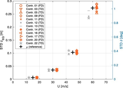
The standard deviation (STD) values of the lateral ($y$), vertical (z) and torsional ($z_{\mathrm{eq}}$) displacement at mid-span increasing the mean wind speed are reported in Figs. 8–10. The torsional values are expressed in equivalent displacement of the deck leading edge as $Z_{\mathrm{eq}}=\left(B/2\right)\theta$.

Fig. 8: STD of lateral displacement at mid-span versus mean wind speed

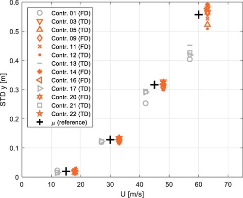
Fig. 9: STD of vertical displacement at mid-span versus mean wind speed

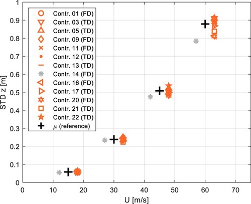
Fig. 10: STD of equivalent torsional displacement at mid-span versus mean wind speed

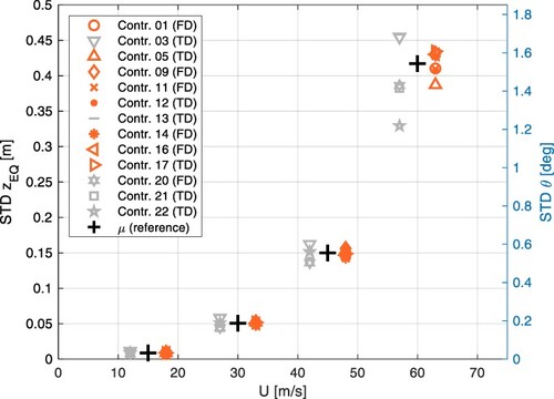
Each figure reports the estimated value as a black cross marker and the contributions that fit within the arbitrary outlier analysis are plotted on the right of the reference in orange. On the other hand, the contributions discarded are plotted on the left in grey. In this case, the criterion was the same as the damping trend with thresholds ${ϵ}_{\mathrm{MAX}}=10\text{\%}$ and ${ϵ}_{\mathrm{mean}}=10\text{\%}$. In the computation of ${ϵ}_{\mathrm{MAX}}$ and ${ϵ}_{\mathrm{mean}}$, the values at 15 m/s are not considered for the STD plots, since they are characterised by a small amplitude of motion deemed negligible in the design of long-span bridges. It is worth pointing out that the contributions, in both orange and grey, still refer to the selected wind speeds (i.e. 15, 30, 45 and 60 m/s) even if they are plotted slightly to the side, in order to improve the readability of the plots.

Results coming from both time domain (TD) and frequency domain (FD) methods are presented. Both TD and FD results show a similar trend and spread. Time domain results (TD) represent the average of the values obtained using the ten randomly produced wind velocity time histories.

Figures 11 through 13 show for completeness the same kind of results for the deck section at the quarter-span station of the main span.

Fig. 11: STD of lateral displacement at quarter-span versus mean wind speed

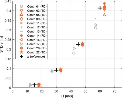
Fig. 12: STD of vertical displacement at quarter-span versus mean wind speed

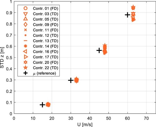
Fig. 13: STD of equivalent torsional displacement at quarter-span versus mean wind speed

Table 5 reports the reference mean value ${\mu }_i$ and the standard deviation ratio ${\sigma }_i/{\mu }_i$ for each selected wind speed at both mid- and quarter-span. Also in this case, the standard deviation ratio results are almost constant and lower than the 10% for each displacement at the wind speeds considered. The only exception occurs at 15 m/s for the lateral ($y$) displacement, at which, however, the mean is very close to zero and thus the value of ${\sigma }_i/{\mu }_i$ is less significant.

Table 5: Estimated values and spread of the accepted contributions for mid-span and quarter-span

			15 m/s	30 m/s	45 m/s	60 m/s
Mid-span	Y	μ (m)	0.019	0.128	0.316	0.557
		σ/μ (%)	19.30	5.14	2.69	4.88
	Z	μ (m)	0.058	0.238	0.508	0.879
		σ/μ (%)	3.76	2.92	3.20	4.42
	zeq	μ (m)	0.009	0.051	0.150	0.417
		σ/μ (%)	5.60	3.26	3.43	3.95
Quarter-span	Y	μ (m)	0.015	0.091	0.225	0.413
		σ/μ (%)	15.86	3.56	1.58	4.24
	Z	μ (m)	0.078	0.296	0.563	0.880
		σ/μ (%)	3.98	2.61	4.07	4.78
	zeq	μ (m)	0.006	0.035	0.103	0.273
		σ/μ (%)	9.18	5.71	4.28	4.10

In addition to the STD trends versus wind speed, additional comparisons can be made for the buffeting response: for FD methods, the comparison of PSDs; for TD methods, the comparison of time histories.

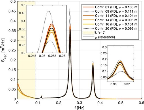
As an example, Figs. 14 and 15 report the power spectral densities (PSDs) of the vertical displacement at mid-span and of the torsional displacement at quarter-span at 45 m/s computed in the frequency domain. For this case, an estimated value is given and plotted as a continuous black line. The usual criterion is adopted with ${ϵ}_{\mathrm{MAX}}=30\text{\%}$ and ${ϵ}_{\mathrm{mean}}=10\text{\%}$, but in this case the deviations between the reference and each contribution are computed over a range of frequencies where PSD values are significant and inside the range where the flutter derivatives are defined. In the legends of Figs. 14 and 15, the STD value for each contribution obtained by numerical integration of the PSD is also reported: these values are the same as those reported in the corresponding plots in Figs. 9 and 13.

Fig. 14: PSD of the vertical displacement at mid-span at 45 m/s of wind mean speed

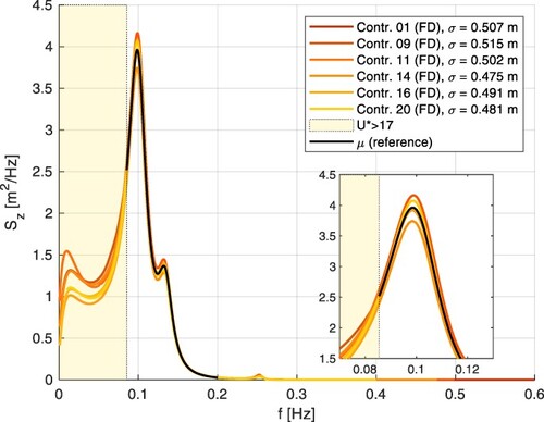
Fig. 15: PSD of the equivalent torsional displacement at quarter-span, at 45 m/s of wind mean speed

A specific comparison for TD results is proposed in Fig. 16, where the time histories of the displacement at mid-span for a wind speed of 45 m/s are reported for the first wind reconstruction (seed 1) of the ten distributed. Simulations are 10 minutes long but, for a better visual comparison, a 60 s window starting at 300 s is shown in the figures.

Fig. 16: Time histories of the vertical displacement z and of the rotation θ at mid-span, at 45 m/s

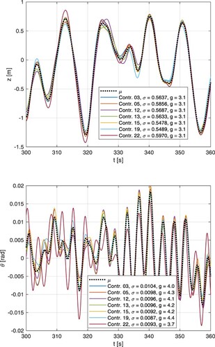
The comparison shows good agreement between all the seven available contributions for vertical displacement, while a larger discrepancy is shown by one of the contributions in the torsional displacement.

To have a more quantitative comparison between the results, some indexes of the metrics reported in Ref. [60] are used as comparisons for the time histories, as shown in Fig. 17. The comparison metrics are constructed in a unified manner using an exponential function with a negative exponent, as follows: (9) $M\left(x,y\right)={\mathrm{e}}^{-\mathrm{\lambda A}\left(x,y\right)}$(9) where $A\left(x,y\right)$ is the relative difference depending on the metric considered,⁶⁰ and λ is a sensitivity parameter taken as one. The relative difference is computed comparing each time history with a reference time history assumed equal the average of all the seven contributions, reported here as dotted black lines. The metrics considered are as follows.

• Phase $\left(M_{\varphi }\right)$, in order to account for the mean phase discrepancy between the selected signal and the reference one.

• Peak $\left(M_p\right)$, to compare the peak value of each time history with respect to the reference. The peak value of the aeroelastic response is an important parameter for the design of long-span bridges.

• Root mean square $\left(M_{\mathrm{rms}}\right)$ is significant as it is closely related to the energy content of the signals.

• Magnitude $\left(M_m\right)$, to determine the local amplitude discrepancies of the time histories.

• Probability density function $\left(M_{\mathrm{pdf}}\right)$ is useful to quantify the non-Gaussian properties of the time histories.

• Frequency content $\left(M_w\right)$ and $\left(M_{\mathrm{wf}}\right)$ using a wavelet analysis, to compare the energy content of two signals in the time–frequency plane.

Fig. 17: Comparison metrics for the vertical displacements (left) and for the rotations (right) at mid-span, at 45 m/s

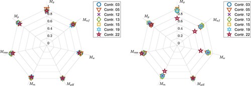
All the metrics are defined explicitly in Ref. [60], which also includes openly available MATLAB^® code. The input parameters for the comparison metrics are given as a MATLAB script in the online supplemental data. The metrics, which are reported in the previous figures in a polar plot, show how the vertical displacement discrepancies are more related to phase and peak values while the torsional displacement differences depends also on the frequency content. For the time histories, good agreement with respect to the reference is expected when all metrics are above the threshold $M\ge 0.8$.

As an additional comment, in the legend of Fig. 16 the value of $g$ is shown, which is the ratio between the peak and the standard deviation $\sigma$ of each contribution. The value of $g$ is approximately three for the vertical displacement and between 3 and 4.5 for the torsional. This value is reported to highlight that TD methods have the advantage over FD methods in that they produce values for the peak responses directly that can be elaborated further by means of extreme value analysis procedures⁶¹ and used for direct derivations of design wind loads.³³

Selected Results for Step B

When the effect of the mean wind speed on the mean bridge displacements is considered in the simulations, the deck rotates changing the mean angle of attack, and consequently the aerodynamic derivatives should be evaluated considering that their values depend on the mean angle of attack. This dependence on angle of attack is the scope of Step B.

To examine the predicted static deformations under mean wind loading using the modal approach, Fig. 18 reports the mean deck rotation as a function of the mean wind speed at mid-span. All contributions are reported in the same manner as in the previous STD plots. The spread of the accepted data, with respect to the estimated mean value ${\mu }_i$, is less than 1% at each mean wind speed, which underlines the good agreement of the selected contributions (Table 6).

Fig. 18: Static rotation at mid-span versus mean wind speed

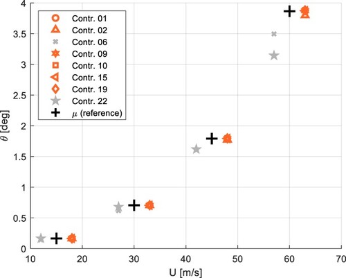
Table 6: Estimated values and spread of the deck static rotation at mid-span

			15 m/s	30 m/s	45 m/s	60 m/s
Mid-span	Θ	μ (deg)	0.165	0.705	1.790	3.864
		σ/μ (%)	0.23	0.12	0.54	0.86

In general, the dependence of the aeroelastic response upon the mean angle of attack is important if there is a strong dependence of the value of the aerodynamic coefficients upon this parameter. As an example, Figs. 19 through 21 report the STD trends for the lateral, vertical and torsional displacements, while the estimated values and their spreads are reported in Table 7. These trends can be compared with those of Step A in Figs. 8 through 10, where the vertical and torsional predictions are very similar, because the relevant lift and moment derivatives do not show an important dependence upon the mean angle of attack. For the lateral displacement, however, at higher wind speeds (i.e. at larger rotations of the deck) there is a significant increase in the response (about two times): this is mainly due to the fact that ${\chi }_{\mathrm{Dw}}^{\ast }=\left(K_D-C_L\right)A\left(V^{\ast }\right)$ passes from ${\chi }_{\mathrm{Dw}}^{\ast }=\left(0.06\right)A\left(V^{\ast }\right)$ at 0° to ${\chi }_{D_w}^{\ast }=\left(0.27\right)A\left(V^{\ast }\right)$ at 4°.

Fig. 19: STD of lateral displacement at mid-span versus mean wind speed

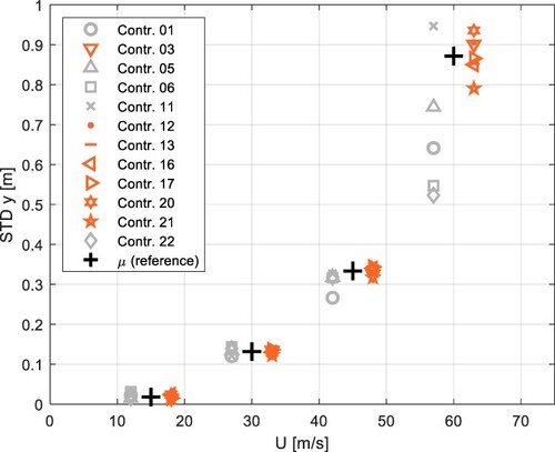
Fig. 20: STD of vertical displacement at mid-span versus mean wind speed

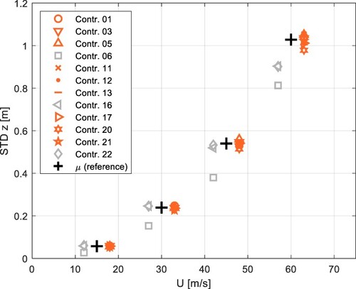
Fig. 21: STD of equivalent torsional displacement at mid-span versus mean wind speed

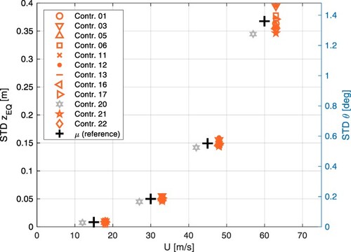
Table 7: Estimated values and spread of accepted contributions for mid-span

			15 m/s	30 m/s	45 m/s	60 m/s
Mid-span	Y	μ (m)	0.018	0.132	0.333	0.872
		σ/μ (%)	24.88	4.10	3.44	5.45
	Z	μ (m)	0.057	0.239	0.540	1.028
		σ/μ (%)	3.35	2.88	2.38	2.55
	zeq	μ (m)	0.008	0.050	0.149	0.368
		σ/μ (%)	18.66	5.55	3.50	4.46

For flutter stability, there is no significant variation of the critical speed, compared to Step A, since for this value the lateral drag force coefficients are less relevant. In this case, the estimated value for flutter speed is $\mu =70.0$ m/s with again ${ϵ}_{\mathrm{MAX}}=2\text{\%}$. However, it should be noted that the mid-span rotation exceeds the +4° aerodynamic derivatives before reaching the flutter speed. Therefore, participants could either extrapolate or directly apply the +4° derivatives when reaching this flutter speed, which potentially may lead to some spread in the predictions.

Conclusions

Thanks to the joint effort of several experts in the field of bridge design, aerodynamics and aeroelasticity, it was possible to set up a benchmark case and to define a range of well estimated results for the aerodynamic stability and buffeting response of long-span bridges. The results presented can be used by anyone to assess and validate their own methodology and numerical procedures, either in the frequency or in the time domain. Two different sets of results are considered, including or excluding the dependence upon the static deck rotation as a function of the mean wind speed.

The following common input data is considered: the first 12 mode shapes and modal parameters for the dynamic description of a suspension bridge; the deck static aerodynamic coefficients as a function of the mean angle of attack; the deck aerodynamic derivatives as a function of the reduced velocity and of the mean angle of attack; the deck admittance function; the power spectra of the turbulent wind field and its spatial coherence functions for frequency domain methods, and a set of time histories of turbulent wind speeds along the deck for time domain methods; the values of mean wind speeds to be investigated.

The results provided in terms of stability are the flutter onset speed and the damping ratio variation of the torsional modal branch. For the buffeting response, the RMS of the displacements as a function of mean wind speed and the PSD values of the displacements for the frequency domain are provided. In addition, for time domain methods, reference time histories of displacements are given. In this article, only key results are presented for brevity, while all input data and detailed calculation results are available in the online supplemental data.

For each estimated result, the authors also present an outlier criterion, which was arbitrarily selected based on the available data. Without claiming that a fully closed solution has been offered, the authors believe that, based on their best efforts, the information given will be useful to others in validating their methodologies and numerical procedures for the wind analysis of long-span bridges.

Disclosure Statement

No potential conflict of interest was reported by the authors.

Supplemental Data

Supplemental data for this article can be accessed online at https://doi.org/10.1080/10168664.2022.2104188.

References

- Diana G, Stoyanoff S, Aas-Jakobsen K, et al. IABSE task group 3.1 benchmark results. part 2: numerical analysis of a three-degree-of-freedom bridge deck section based on experimental aerodynamics. Struct Eng Int. 2020;30(3):411–420. DOI:10.1080/10168664.2019.1661331.
- Diana G, Stoyanoff S, Aas-Jakobsen K, et al. IABSE task group 3.1 benchmark results. part 1: numerical analysis of a two-degree-of-freedom bridge deck section based on analytical aerodynamics. Struct Eng Int. 2020;30(3):401–410. DOI:10.1080/10168664.2019.1639480.
- Wu T, Kareem A. Bridge aerodynamics and aeroelasticity: a comparison of modeling schemes. J Fluids Struct. 2013;43:347–370. DOI:10.1016/j.jfluidstructs.2013.09.015.
- Strømmen EN. Theory of bridge aerodynamics. 2nd ed. Berlin, Heidelberg: Springer, 2010.
- Jain A, Jones NP, Scanlan RH. Coupled flutter and buffeting analysis of long-span bridges. J Struct Eng New York, N.Y. 1996;122(7):716–725. DOI:10.1061/(ASCE)0733-9445(1996)122:7(716).
- Davenport AG. The response of slender, line-like structures to a gusty wind. Proce Inst Civil Eng. 1962;23(3):389–408.
- Davenport AG. Buffeting of a suspension bridge by storm winds. J Struct Div. 1962;88(3):233–268.
- Irwin PA. Wind tunnel and analytical investigation of the response of lion’s gate bridge to a turbulent wind. LTR-LA-210. Ottawa: National Research Council Canada; 1977.
- Beliveau J, Vaicaitis R, Shinozuka M. Motion of suspension bridge subject to wind loads. J Struct Division. 1977;103(6):1189–1205.
- Solari G, Spinelli P. Time-domain analysis of tall buildings response to wind action. 1984.
- Hao J, Wu T. Downburst-induced transient response of a long-span bridge: a CFD-CSD-based hybrid approach. J Wind Eng Ind Aerodyn. 2018;179:273–286. DOI:10.1016/j.jweia.2018.06.006.
- Hao J, Wu T. Nonsynoptic wind-induced transient effects on linear bridge aerodynamics. J Eng Mech. 2017;143(9). DOI:10.1061/(ASCE)EM.1943-7889.0001313.
- Wu T, Kareem A. A nonlinear analysis framework for bluff-body aerodynamics: a Volterra representation of the solution of navier-stokes equations. J Fluids Struct. 2015;54:479–502. DOI:10.1016/j.jfluidstructs.2014.12.005.
- Diana G, Rocchi D, Argentini T. An experimental validation of a band superposition model of the aerodynamic forces acting on multi-box deck sections. J Wind Eng Ind Aerodyn. 2013;113:40–58. DOI:10.1016/j.jweia.2012.12.005.
- Wu T, Kareem A, Ge Y. Linear and nonlinear aeroelastic analysis frameworks for cable-supported bridges. Nonlinear Dyn. 2013;74(3):487–516. DOI:10.1007/s11071-013-0984-7.
- Argentini T, Diana G, Rocchi D, Somaschini C. A case-study of double multi-modal bridge flutter: experimental result and numerical analysis. J. Wind Eng. Ind. Aerodyn. 2016;151:25–36. doi:10.1016/j.jweia.2016.01.004.
- Diana G, Omarini S. A non-linear method to compute the buffeting response of a bridge validation of the model through wind tunnel tests. J Wind Eng Ind Aerodyn. 2020;201. DOI:10.1016/j.jweia.2020.104163.
- Wu T, Kareem A. A nonlinear convolution scheme to simulate bridge aerodynamics. Comput Struct. 2013;128:259–271. DOI:10.1016/j.compstruc.2013.06.004.
- Skyvulstad H, Argentini T, Zasso A, Øiseth O. Nonlinear modelling of aerodynamic self-excited forces: an experimental study. J Wind Eng Ind Aerodyn. 2021;209. DOI:10.1016/j.jweia.2020.104491.
- Skyvulstad H, Petersen ØW, Argentini T, Zasso A, Øiseth O. The use of a Laguerrian expansion basis as Volterra kernels for the efficient modeling of nonlinear self-excited forces on bridge decks. J Wind Eng. Ind. Aerodyn. 2021;219. DOI:10.1016/j.jweia.2021.104805.
- Stoyanoff S. A unified approach for 3D stability and time domain response analysis with application of quasi-steady theory. J Wind Eng Ind Aerodyn. 2001;89(14–15):1591–1606. DOI:10.1016/S0167-6105(01)00157-X.
- Kavrakov I, McRobie A, Morgenthal G. Data-driven aerodynamic analysis of structures using gaussian processes; 2021.
- Argentini T, Rocchi D, Somaschini C. Effect of the low-frequency turbulence on the aeroelastic response of a long-span bridge in wind tunnel. J Wind Eng Ind Aerodyn. 2020;197. DOI:10.1016/j.jweia.2019.104072.
- Diana G, Rocchi D, Argentini T, Muggiasca S. Aerodynamic instability of a bridge deck section model: linear and nonlinear approach to force modeling. J Wind Eng Ind Aerodyn. 2010;98(6–7):363–374. DOI:10.1016/j.jweia.2010.01.003.
- Kavrakov I, Morgenthal G. A synergistic study of a CFD and semi-analytical models for aeroelastic analysis of bridges in turbulent wind conditions. J Fluids Struct. 2018;82:59–85. DOI:10.1016/j.jfluidstructs.2018.06.013.
- Bućher CG, Lin YK. Stochastic stability of bridges considering coupled modes: II. J Eng Mech. 1989;115(2):384–400. DOI:10.1061/(ASCE)0733-9399(1989)115:2(384).
- Chen X, Matsumoto M, Kareem A. Time domain flutter and buffeting response analysis of bridges. J Eng Mech. 2000;126(1):7–16. DOI:10.1061/(ASCE)0733-9399(2000)126:1(7).
- Kavrakov I, Morgenthal G. A comparative assessment of aerodynamic models for buffeting and flutter of long-span bridges. Engineering. 2017;3(6):823–838. DOI:10.1016/j.eng.2017.11.008.
- Øiseth O, Sigbjörnsson R. An alternative analytical approach to prediction of flutter stability limits of cable supported bridges. J Sound Vibrat. 2011;330(12):2784–2800. DOI:10.1016/j.jsv.2010.12.026.
- Øiseth O, Rönnquist A, Sigbjörnsson R. Finite element formulation of the self-excited forces for time-domain assessment of wind-induced dynamic response and flutter stability limit of cable-supported bridges. Finite Elements Anal Des. 2012;50:173–183. DOI:10.1016/j.finel.2011.09.008.
- Øiseth O, Rönnquist A, Sigbjörnsson R. Simplified prediction of wind-induced response and stability limit of slender long-span suspension bridges, based on modified quasi-steady theory: a case study. J Wind Eng Ind Aerodyn. 2010;98(12):730–741. DOI:10.1016/j.jweia.2010.06.009.
- Øiseth O, Rönnquist A, Sigbjörnsson R. Time domain modeling of self-excited aerodynamic forces for cable-supported bridges: a comparative study. Computers and Structures. 2011;89(13–14):1306–1322. DOI:10.1016/j.compstruc.2011.03.017.
- Stoyanoff S, Dallaire PO. A direct method for calculation of wind loads on LongSpan bridges. In: 12th Americas Conference on Wind Engineering 2013, ACWE 2013: Wind Effects on Structures, Communities, and Energy Generation, 2013. p. 1316–1325.
- Park J, Jung K, Hong YH, Kim H, Lee HS. Exact enforcement of the causality condition on the aerodynamic impulse response function using a truncated Fourier series. J Eng Mech. 2014;140(5). doi:10.1061/(ASCE)EM.1943-7889.0000721.
- Jung K, Kim H, Lee HS. New unified approach for aeroelastic analyses using approximate transfer functions of aerodynamic forces. J Eng Mech. 2014;140(4). doi:10.1061/(ASCE)EM.1943-7889.0000716.
- Jung K, Kim H, Lee HS. Evaluation of impulse response functions for convolution integrals of aerodynamic forces by optimization with a penalty function. J Eng Mech. 2012;138(5):519–529. DOI:10.1061/(ASCE)EM.1943-7889.0000355.
- Matsumoto M, Okubo K, Ito Y, Matsumiya H, Kim G. The complex branch characteristics of coupled flutter. J Wind Eng Ind Aerodyn. 2008;96(10–11):1843–1855. DOI:10.1016/j.jweia.2008.02.011.
- Møller RN, Krenk S, Svendsen MN. Time simulation of aerodynamic response of long-span bridges to turbulent wind. J Wind Eng Ind Aerodyn. 2020;199. DOI:10.1016/j.jweia.2019.104060.
- Argentini T, Pagani A, Rocchi D, Zasso A. Monte Carlo analysis of total damping and flutter speed of a long span bridge: effects of structural and aerodynamic uncertainties. J Wind Eng Ind Aerodyn. 2014;128:90–104. DOI:10.1016/j.jweia.2014.02.010.
- Chen X, Kareem A, Matsumoto M. Multimode coupled flutter and buffeting analysis of long span bridges. J Wind Eng Ind Aerodyn. 2001;89(7–8):649–664. DOI:10.1016/S0167-6105(01)00064-2.
- Diana G, Rocchi D, Argentini T. Buffeting response of long span bridges: numerical-experimental validation of fluid-structure interaction models. In: IABSE conference, Geneva 2015: Structural Engineering: Providing Solutions to Global Challenges – Report; 2015. https://www.scopus.com/record/display.uri?eid=2-s2.0-84971301417&origin=resultslist.
- Cid Montoya M, Hernández S, Nieto F, Kareem A. Aero-structural design of bridges focusing on the buffeting response: formulation, parametric studies and deck shape tailoring. J Wind Eng Ind Aerodyn. 2020;204. doi:10.1016/j.jweia.2020.104243.
- Wu T, Kareem A. Revisiting convolution scheme in bridge aerodynamics: comparison of step and impulse response functions. J Eng Mech. 2014;140(5). doi:10.1061/(ASCE)EM.1943-7889.0000709.
- Kavrakov I, Legatiuk D, Gürlebeck K, Morgenthal G. A categorical perspective towards aerodynamic models for aeroelastic analyses of bridge decks. R Soc Open Sci. 2019;6(3). DOI:10.1098/rsos.181848.
- Hodges DH, Pierce GA. Introduction to structural dynamics and aeroelasticity, second edition. In: Introduction to Structural Dynamics and Aeroelasticity, 2nd ed. 2011. doi:10.1017/CBO9780511997112.
- Scanlan RH. The action of flexible bridges under wind, II: buffeting theory. J. Sound Vibrat. 1978;60(2):201–211. DOI:10.1016/S0022-460X(78)80029-7.
- Argentini T, Rocchi D, Somaschini C, Spinelli U, Zanelli F, Larsen A. Aeroelastic stability of a twin-box deck: comparison of different procedures to assess the effect of geometric details. J Wind Eng Ind Aerodyn. 2022;220. DOI:10.1016/j.jweia.2021.104878.
- Larsen A. Aerodynamic aspects of the final design of the 1624 m suspension bridge across the great belt. J Wind Eng Ind Aerodyn. 1993;48(2–3):261–285. DOI:10.1016/0167-6105(93)90141-A.
- COWI, BHR and R&H. Storebælt east bridge tender design, dynamic analyses. (Doc. No. 2000-X012-001), 1992.
- Katsuchi H, Jones NP, Scanlan RH. Multimode coupled flutter and buffeting analysis of the Akashi-Kaikyo bridge. J Struct Eng. 1999;125(1):60–69. DOI:10.1061/(asce)0733-9445(1999)125:1(60).
- Deodatis G. Simulation of Ergodic multivariate stochastic processes. J Eng Mech. 1996;122(8):778–787. DOI:10.1061/(ASCE)0733-9399(1996)122:8(778).
- Ding Q, Zhu L, Xiang H. Simulation of stationary Gaussian stochastic wind velocity field. Wind Struct Int J. 2006;9(3):231–243. DOI:10.12989/was.2006.9.3.231.
- Shinozuka M, Jan C. Digital simulation of random processes and its applications. J Sound Vibrat. 1972;25(1):111–128. DOI:10.1016/0022-460X(72)90600-1.
- Diana G, et al. Flutter derivatives identification on a very large scale aeroelastic deck model. In: IABSE conference, Vancouver 2017: engineering the future – report; 2017. p. 1997–2005.
- Zasso A. Flutter derivatives: advantages of a new representation convention. J Wind Eng Ind Aerodyn. 1996;60(1–3):35–47. DOI:10.1016/0167-6105(96)00022-0.
- Diana G, Bruni S, Cigada A, et al. Turbulence effect on flutter velocity in long span suspended bridges. J Wind Eng Ind Aerodyn. 1993;48(2):329–342. doi:10.1016/0167-6105(93)90144-D.
- Diana G, Cheli F, Zasso A, et al. Suspension bridge parameter identification in full scale test. J. Wind Eng. Ind. Aerodyn. 1992;41(1):165–176. doi:10.1016/0167-6105(92)90404-X.
- Diana G, Resta F, Zasso A, et al. Forced motion and free motion aeroelastic tests on a new concept dynamometric section model of the Messina suspension bridge. J. Wind Eng. Ind. Aerodyn. 2004;92(6):441–462. DOI:10.1016/j.jweia.2004.01.005.
- Scanlan RH. Motion-related body-force functions in two-dimensional low-speed flow. J Fluids Struct. 2000;14(1):49–63. doi:10.1006/jfls.1999.0252.
- Kavrakov I, Kareem A, Morgenthal G. Comparison metrics for time-histories: application to bridge aerodynamics. J Eng Mech. 2020;146(9). doi:10.1061/(ASCE)EM.1943-7889.0001811.
- Cook NJ, Mayne JR. A refined working approach to the assessment of wind loads for equivalent static design. J Wind Eng Ind Aerodyn. 1980;6(1):125–137. doi:10.1016/0167-6105(80)90026-4.