A diluted version of the problem of the existence of the Hofstadter sequence

Abstract

We investigate the conditions on an integer sequence $f(n)$, $n\in \mathbb{N}$, with $f(1)=0$, such that the sequence $q(n)$, computed recursively via $q(n)=q(n-q(n-1))+f(n)$, with $q(1)=1$, exists. We prove that $f(n)$ is ‘slow’, that is, $f(n+1)-f(n)\in \{0,1\}$, $n\ge 1$, is a sufficient but not necessary condition for the existence of sequence q. Sequences q defined in this way typically display non-trivial dynamics: in particular, they are generally aperiodic with no obvious patterns. We discuss and illustrate this behavior with some examples.

Keywords:

• Nested recursion
• Hofstadter q-sequence
• existence of solutions
• nonlinear dynamics

2020 Mathematics Subject Classifications:

• 11B37
• 11B39

1. Motivation

In his 1979 book [3], author D.R. Hofstadter mentions an integer sequence, $q_h(n)$, defined, for n>2, by (1) $q_h(n)=q_h(n-q_h(n-1))+q_h(n-q_h(n-2))\mathrm{with}{q}_h(1)=q_h(2)=1.$(1) In order for $q_h(n)$ to exist for all positive integers n, that is, for $n\in \mathbb{N}$, it must be true, again for all $n\in \mathbb{N}$, that $1\le q_h(n)\le n$, since only then does the right-hand side of (1(1) $q_h(n)=q_h(n-q_h(n-1))+q_h(n-q_h(n-2))\mathrm{with}{q}_h(1)=q_h(2)=1.$(1) ) refer to terms that are already known: $q_h(n)$ is undefined for $n\le 0$. Should it happen that $q_h(n)>n$ for some n, the sequence is said to die at n. Although direct computation shows that $q_h(n)$ exists for $1\le n\le 3\times {10}^{10}$ [5], the existence of $q_h(n)$ for all positive n is still an open question.

The sequence $q_h(n)$ is non-monotonic, aperiodic and its dynamical behavior appears to be complex. In [9] for instance, small scale ‘chaotic’ behavior is described, with some order apparent at larger scales, and several statistical properties of the sequence are also investigated.

This complex behavior has inspired several authors to study variations of Hofstadter's original recursion. For instance, Tanny [11] considers $T(n)=T(n-1-T(n-1))+T(n-2-T(n-2))\mathrm{with}T(0)=T(1)=T(2)=1,$for n>2 [6]. Another variant is considered in [1], in which the authors investigate $V(n)=V(n-V(n-1))+V(n-V(n-4))\mathrm{with}V(1)=V(2)=V(3)=V(4)=1$for n>4 [7]. Both these variants give rise to sequences that are monotonic, unlike $q_h(n)$, and hit every positive integer.

A different approach is followed in [2], in which the recursion formula in (1(1) $q_h(n)=q_h(n-q_h(n-1))+q_h(n-q_h(n-2))\mathrm{with}{q}_h(1)=q_h(2)=1.$(1) ) is retained but different initial conditions are used. For certain initial conditions, ‘eventually quasi-polynomial’ solutions can be found. For a given integer m>0 and a given fixed set of polynomials $p_i(n)$, $i=0,\dots ,m-1$, a quasi-polynomial function of n, $h(n)$, say, is defined by $h(n)=p_i(n)$, where $i=nmodm$. If this holds only for n greater than some positive integer $n_0$ say, then $h(n)$ is said to be eventually quasi-polynomial. In [2], families of eventually quasi-polynomial solutions to (2) $r(n)=r(n-r(n-1))+r(n-r(n-2)),$(2) with suitable initial conditions, are constructed. As an example of such a solution with m = 5 and where the $p_i(n)$ are of degree at most 1, we give $\begin{array}{llllll}i& 0& 1& 2& 3& 4\\ p_i(n)& 2& n-4& 5& n-5& n-6,\end{array}$

along with the initial conditions $r(3),\dots ,r(12)=1,1,3,5,1,4,7,6,4,9$. (Values of $r(1)$ and $r(2)$ are not needed to compute $r(n),n>2$.) For all $n>n_0=12$ here, $r(n)$ satisfying (2(2) $r(n)=r(n-r(n-1))+r(n-r(n-2)),$(2) ) is then given by the quasi-polynomial above.

In this paper, we also consider a variation on the original problem, one which consists of an infinite number of variants rather than just a single case. In particular, we discuss a ‘diluted’ version of the problem of the existence of $q_h(n)$. In order to describe this version, we first need the notation $(a(n){)}_{n\in \mathbb{N}}:=a(1),a(2),\dots$ for an infinite sequence. We use this notation in formal contexts, such as in definitions and lemmas, but where it it is clear what is intended, we just write a to mean the whole sequence. Naturally, when the nth term is meant, we write $a(n)$. We also need the following definitions:

Definition 1.1

Slow sequence

If integer sequence $(a(n){)}_{n\in \mathbb{N}}$ obeys $a(n+1)-a(n)\in \{0,1\}$ for $n\in \mathbb{N}$, then the sequence is said to be ‘slow’.

Definition 1.2

Property ${\mathrm{S}}_0$

If integer sequence $(a(n){)}_{n\in \mathbb{N}}$ is slow and additionally $a(1)=0$, then it is said to have property ${\mathrm{S}}_0$.

We drop the quotation marks around the word ‘slow’ from now on.

The problem that we consider is the question of the existence of sequences q defined recursively by (3) $q(n)=q(n-q(n-1))+f(n)\mathrm{with}q(1)=1,$(3) for $n\in \mathbb{N}$, n>1, and where $f(n)$ has property ${\mathrm{S}}_0$ (so in particular $f(1)=0$). All sequences in the paper start from index 1 and we apply the conditions $q(1)=1$ and $f(1)=0$ strictly throughout, even though $f(1)$ is never needed to compute the sequence q. Computations suggest that, under these conditions, the sequence q corresponding to any f with property ${\mathrm{S}}_0$ exists for all $n\in \mathbb{N}$.

We think of sequences generated by (3(3) $q(n)=q(n-q(n-1))+f(n)\mathrm{with}q(1)=1,$(3) ) as ‘diluted’ Hofstadter sequences because of the similarity of their definition to that of the original $q_h$-sequence. In particular, in (3(3) $q(n)=q(n-q(n-1))+f(n)\mathrm{with}q(1)=1,$(3) ), one ‘difficult’ – nested – term is retained, $q(n-q(n-1))$, but the second nested term is replaced by $f(n)$, which is under our control.

Clearly the existence of the sequence q is also equivalent to the inequality $1\le q(n)\le n$ holding for all $n\in \mathbb{N}$. If this is the case, then we simply say that q exists. The lower bound on $q(n)$ here is easy: by (3(3) $q(n)=q(n-q(n-1))+f(n)\mathrm{with}q(1)=1,$(3) ), for any n for which q exists, $q(n)$ is the sum of a positive integer and a non-negative one, and so is also greater than or equal to unity.

The upper bound on q, however, is less obvious. In what follows, after some preliminaries, we give a proof of the following theorem.

Theorem 1.3

For all sequences $(f(n){)}_{n\in \mathbb{N}}$ having property ${\mathrm{S}}_0$, the corresponding sequence $(q(n){)}_{n\in \mathbb{N}}$ with $q(1)=1$ and with $q(n)$, for n>1, computed from (3(3) $q(n)=q(n-q(n-1))+f(n)\mathrm{with}q(1)=1,$(3) ), exists for all $n\in \mathbb{N}$.

The proof of this theorem is the main result of the paper, but the recursion (3(3) $q(n)=q(n-q(n-1))+f(n)\mathrm{with}q(1)=1,$(3) ) can also be viewed as a non-linear (in the light of the nested term), non-autonomous (because of $f(n)$) dynamical system, discrete in both time and space. Hence, having proved the existence of q for all f with property ${\mathrm{S}}_0$, we make some observations about the dynamics of sequences q, which are also interesting.

2. Preliminaries

The first term of all sequences in this paper has index 1. We start by giving the following definitions:

• Two sequences $(a(n){)}_{n\in \mathbb{N}}$ and $(b(n){)}_{n\in \mathbb{N}}$ differ if there exists $n^{\prime }\in \mathbb{N}$ such that $a(n^{\prime })\ne b(n^{\prime })$; otherwise, they are equal.

• A sequence $(q(n){)}_{n\in \mathbb{N}}$ obeying (3(3) $q(n)=q(n-q(n-1))+f(n)\mathrm{with}q(1)=1,$(3) ) exists if and only if $q(n)$ is defined for all $n\in \mathbb{N}$; or, equivalently, if $1\le q(n)\le n$ for all $n\in \mathbb{N}$.

• A sequence $Q(f):=(q(n){)}_{n\in \mathbb{N}}$ is the sequence corresponding to sequence $(f(n){)}_{n\in \mathbb{N}}$ if $(q(n){)}_{n\in \mathbb{N}}$ exists and is defined by (3(3) $q(n)=q(n-q(n-1))+f(n)\mathrm{with}q(1)=1,$(3) ).

• A sequence $F(q):=(f(n){)}_{n\in \mathbb{N}}$ is the sequence corresponding to sequence $(q(n){)}_{n\in \mathbb{N}}$ if $(q(n){)}_{n\in \mathbb{N}}$ exists and $f(n)$ is defined by $f(1)=0$ and $f(n)=q(n)-q(n-q(n-1))$ for n>1.

Where an explicit expression for $f(n)$ is available, for example $f(n)=\lfloor n/2\rfloor$, we may write $Q(\lfloor n/2\rfloor )$.

Where we need to refer explicitly to the first few terms of a sequence, $a(n)$ say, we list the values starting from $a(1)$ – for example $a=(1,2,4,4)$ means $a(1)=1$, $a(2)=2$, $a(3)=a(4)=4$.

Let us define $\mathcal{S}$ as the set of all sequences having property ${\mathrm{S}}_0$: that is $\mathcal{S}:=\{(f(n){)}_{n\in \mathbb{N}}:f(1)=0,f(i+1)-f(i)\in \{0,1\}\text{for}i\in \mathbb{N}\}.$We will also need the set of finite sequences with property ${\mathrm{S}}_0$: ${\mathcal{S}}_m:=\{{(f(n))}_{n=1,\dots ,m}:f(1)=0,f(i+1)-f(i)\in \{0,1\}\text{for}i=1,\dots ,m-1\}.$It is easily established that the cardinality of $\mathcal{S}$ is the same as that of the real numbers. To do so, let $f\in \mathcal{S}$ and consider the sequence of differences $(f(i+1)-f(i){)}_{i\in \mathbb{N}}$, which will be a sequence consisting of the symbols 0 and 1. Interpreting this as a binary decimal, we see that each distinct $f\in \mathcal{S}$ gives rise to a distinct real number $x\in [0,1]$.

One important subset of $\mathcal{S}$, with same cardinality, is $\mathcal{G}:=\{(f(n){)}_{n\in \mathbb{N}}=\lfloor \mathrm{\alpha n}\rfloor \mathrm{with}\alpha \in [0,1)\}.$

It is easy to see (i) that $\mathcal{G}\subset \mathcal{S}$, and that in fact (ii) $\mathcal{G}⊊\mathcal{S}$. Property (i) comes directly from the definition $\lfloor x\rfloor :=max\{k\in \mathbb{Z}:k\le x\}$, from which we deduce that, for $\alpha \in [0,1]$, $\lfloor \alpha (n+1)\rfloor -\lfloor \mathrm{\alpha n}\rfloor$ is either 0 or 1. For property (ii), consider the sequence $a(1),\dots ,a(4)=0,0,1,2$, which are the first four terms of a sequence in $\mathcal{S}$. Now assume that these terms are generated by $a(n)=\lfloor \mathrm{\alpha n}\rfloor$ for some α. Then $a(2)=0$ implies that $\alpha \in [0,1/2)$, but $a(4)=2$ implies that $\alpha \in [1/2,3/4)$, leading to a contradiction. Hence, there are sequences in $\mathcal{S}$ that are not in $\mathcal{G}$.

Furthermore, the condition that successive terms in a sequence $f(n)$ differ by at most unity turns out to be sufficient but not necessary for the corresponding $(q(n){)}_{n\in \mathbb{N}}$ to exist. There are examples where f increases by more than unity, and where it is not monotonic, but for which $Q(f)$ nonetheless exists. Consider, for instance, (a) $f_a=(0,0,2,2,4,4,\dots )$, for which $q_a=Q(f_a)=(1,1,3,3,5,5,\dots )$ and (b) $f_b=(0,1,0,1,0,1,\dots )$, for which $q_b=Q(f_b)=(1,2,1,2,1,2,\dots )$. Statements (a) and (b) are proved in

Lemma 2.1

If $f_a(n)=2\lfloor \frac{n-1}{2}\rfloor =n-\frac{3+(-1{)}^n}{2},\mathrm{then}{q}_a(n)=n-\frac{1+(-1{)}^n}{2}$and if $f_b(n)=\frac{1+(-1{)}^n}{2},\mathrm{then}{q}_b(n)=\frac{3+(-1{)}^n}{2}$for all $n\in \mathbb{N}.$

Proof.

These just boil down to computation.

For $q_a$, we have $n-q_a(n-1)=\{\begin{array}{ll}1& n\mathrm{is}\mathrm{even}\\ 2& n\mathrm{is}\mathrm{odd},\end{array}$so $q_a(n-q_a(n-1))=1$ for all n. Hence, $q_a(n)-q_a(n-q_a(n-1))=q_a(n)-1=n-\frac{3+(-1{)}^n}{2}=f_a(n)$, as claimed.

For $f_b$, we have $n-q_b(n-1)=\{\begin{array}{ll}n-1& n\mathrm{is}\mathrm{even}\\ n-2& n\mathrm{is}\mathrm{odd}.\end{array}$Hence, $n-q_b(n-1)$ is odd, and so $q_b(n-q_b(n-1))=1$, both for all n. Therefore, $q_b(n)-q_b(n-q_b(n-1))=q_b(n)-1=\frac{1+(-1{)}^n}{2}=f_b(n)$.

Remark 2.2

Example (b) is in fact a special case of $\mathrm{If}m\in \mathbb{N}\mathrm{and}f(n)=(n-1)modm,\mathrm{then}q(n)=f(n)+1=((n-1)modm)+1.$

On the other hand, it is easy to find examples of $f\notin \mathcal{S}$ for which $Q(f)$ does not exist – for instance, $f=(0,2,2)$, for which $q(1)=1,q(2)=3$ and so $q(3)=q(0)+f(3)$ which is undefined.

We also prove

Lemma 2.3

If f and $f^{\prime }$ are different sequences, and $Q(f)$ and $Q(f^{\prime })$ both exist, then $Q(f)\ne Q(f^{\prime })$.

Proof.

Let $f(n)=f^{\prime }(n)$ for $1\le n\le k$ but $f(k+1)\ne f^{\prime }(k+1)$. Write $q=Q(f)$, $q^{\prime }=Q(f^{\prime })$. Now, $q(n)=q^{\prime }(n)$ for $1\le n\le k$ and $q(k+1)=q(k+1-q(k))+f(k+1)$, $q^{\prime }(k+1)=q^{\prime }(k+1-q^{\prime }(k))+f^{\prime }(k+1)$. Also, $k+1-q(k)=k+1-q^{\prime }(k)$, but $f(k+1)\ne f^{\prime }(k+1)$. Hence $q(k+1)\ne q^{\prime }(k+1)$ and so the sequences q, $q^{\prime }$ differ.

We remark here that the recursion (3(3) $q(n)=q(n-q(n-1))+f(n)\mathrm{with}q(1)=1,$(3) ) can be used in either direction. That is, given any sequence f for which $q=Q(f)$ exists, sequence q can obviously be computed, term-by-term, in order of increasing index, from (3(3) $q(n)=q(n-q(n-1))+f(n)\mathrm{with}q(1)=1,$(3) ); and, given any sequence q obeying $1\le q(n)\le n$ for all n, (3(3) $q(n)=q(n-q(n-1))+f(n)\mathrm{with}q(1)=1,$(3) ) can be used to compute $f(n)$ for all n. A case where computing f given q gives an interesting result is

Lemma 2.4

Let sequence $q(n)$ obey (i) $1\le q(n)\le n$ and (ii) $q(n+1)-q(n)\in \{0,1\}$, both for $n\in \mathbb{N}$, and let $q(1)=1$. Define $f(n)=q(n)-q(n-q(n-1))$ for $n\ge 2$ with $f(1)=0$. Then, for $n\ge 1$, $f(n+1)-f(n)\in \{-1,0,1\}$.

Proof.

Throughout the proof, we assume integer $n\ge 2$. Assumption (i) tells us that q exists and (ii), that q is slow. By the definition of $f(n)$, $f(n+1)-f(n)=\underset{:=A(n)}{\underbrace{q(n+1)-q(n)}}-\underset{:=B(n)}{\underbrace{[q(n+1-q(n))-q(n-q(n-1))]}}.$Assumption (ii) implies immediately that $A(n)\in \{0,1\}$.

Now define $\ell (n):=n-q(n-1)$: by (i), $1\le \ell (n)\le n-1$. Then $\ell (n+1)-\ell (n)=1-(q(n)-q(n-1))\in \{0,1\}$, again by (ii). Hence, $B(n)$ is either $q(\ell (n))-q(\ell (n))=0$, or $q(\ell (n)+1)-q(\ell (n))\in \{0,1\}$. Therefore, $B(n)\in \{0,1\}$. Thus we have $A(n)-B(n)\in \{-1,0,1\}$ and the lemma is proven.

Note that the converse of Lemma 2.4 is not true: if $f(n+1)-f(n)\in \{-1,0,1\}$ then q is not necessarily slow: a counterexample is given by $f_b$ in Lemma 2.1.

Finally, we point out that cases in which $f\in \mathcal{S}$ gives rise to a monotonic sequence q appear to be rare – a few examples, each of which is also slow, are given in Section 4.

3. The main theorem

We now give a proof of Theorem 1.3. We need several lemmas, the first of which is

Lemma 3.1

The shift property

Let $(f(n){)}_{n\in \mathbb{N}}$, with $f(1)=0$, be any sequence of integers for which the corresponding sequence $(q(n){)}_{n\in \mathbb{N}}=Q(f)$, with $q(1)=1$, exists. Define $(f^{\prime }(n){)}_{n\in \mathbb{N}}:=\{\begin{array}{ll}0& n=1\\ f(n-1)& n>1\end{array}\mathrm{and}(q^{\prime }(n){)}_{n\in \mathbb{N}}:=\{\begin{array}{ll}1& n=1\\ q(n-1)& n>1\end{array}.$Then we have that $(\mathrm{A})q=Q(f)$ implies $q^{\prime }=Q(f^{\prime })$ and $(\mathrm{B})f=F(q)$ implies $f^{\prime }=F(q^{\prime })$.

Proof.

A ⇒ B. We use strong induction and the fact that both q and $q^{\prime }$ obey (3(3) $q(n)=q(n-q(n-1))+f(n)\mathrm{with}q(1)=1,$(3) ).

First, $q(1)=q^{\prime }(1)=1$ by definition, and $q^{\prime }(2)=q^{\prime }(2-q^{\prime }(1))+f^{\prime }(2)=1+f(1)=1$. Hence, $q^{\prime }(2)=q(1)$.

Next, assume that (4) $q^{\prime }(n)=q(n-1)\mathrm{for}n=3,\dots ,k\mathrm{with}k>3.$(4) Now, by assumption (4(4) $q^{\prime }(n)=q(n-1)\mathrm{for}n=3,\dots ,k\mathrm{with}k>3.$(4) ), we have that $q^{\prime }(k)=q(k-1)$. For the inductive step $k\mapsto k+1$, we have that $\begin{array}{rl}{q}^{\prime }(k+1)-q(k)& =q^{\prime }(k+1-q^{\prime }(k))-q(k-q(k-1))\\ & =q^{\prime }(k+1-q(k-1))-q(k-q(k-1))=q^{\prime }(m+1)-q(m),\end{array}$where $m=k-q(k-1)$. We have $2\le m+1\le k$, since q exists, and so, by (4(4) $q^{\prime }(n)=q(n-1)\mathrm{for}n=3,\dots ,k\mathrm{with}k>3.$(4) ), $q^{\prime }(m+1)=q(m)$ and hence $q^{\prime }(k+1)=q(k)$.

B ⇒ A. This is straightforward. By definition, we have $f^{\prime }(1)=0$. Then, by B, we have $q^{\prime }(1)=1$ and $q^{\prime }(2)=q(1)=1$. Hence, by (3(3) $q(n)=q(n-q(n-1))+f(n)\mathrm{with}q(1)=1,$(3) ), $f^{\prime }(2)=q^{\prime }(2)-q^{\prime }(2-q^{\prime }(1))=0$. Then, letting $n\ge 3$, we have $f^{\prime }(n)=q^{\prime }(n)-q^{\prime }(n-q^{\prime }(n-1))=q(n-1)-q(n-1-q(n-2))=f(n-1),$as claimed. Here we have used B and (3(3) $q(n)=q(n-q(n-1))+f(n)\mathrm{with}q(1)=1,$(3) ) for the second-last and last equalities respectively.

We will also need the following two special cases of $f\in \mathcal{S}$, each of which, unusually, leads to a slow sequence q:

Lemma 3.2

Let $f_0(n)=0$ and $f_1(n)=n-1$, both for all $n\in \mathbb{N}$, and define sequences $q_0=Q(f_0)$, $q_1=Q(f_1)$. Then $q_0(n)=1$ and $q_1(n)=n$, also for all n.

Proof.

For $q_0(n)$, (3(3) $q(n)=q(n-q(n-1))+f(n)\mathrm{with}q(1)=1,$(3) ) gives $q_0(n)=q_0(n-q_0(n-1))$ since $f_0(n)=0$. By induction, with base case $q_0(1)=1$, we make the assumption that for some k>1 we have $q_0(k)=1$. Then, by the recursion formula, we have $q_0(k+1)=q_0(k+1-q_0(k))=q_0(k)=1$, as claimed.

For $q_1(n)$, (3(3) $q(n)=q(n-q(n-1))+f(n)\mathrm{with}q(1)=1,$(3) ) gives $q_1(n)=q_1(n-q_1(n-1))+n-1$ since $f_1(n)=n-1$. With $q_1(1)=1$, we assume that $q_1(k)=k$ for some k>1. Then $q_1(k+1)=q_1(k+1-q_1(k))+k=q_1(1)+k=k+1$and the proof is complete.

In the remainder of this section, f will always have property ${\mathrm{S}}_0$ and we will assume that f is such that $Q(f)$ exists. We introduce the handy notation $\{j:k\}$, with $k\ge j$, to designate the set of successive integers $\{j,j+1,\dots ,k\}$.

We now consider the question: for a particular n, given that $f(n)=i\in \{0:n-1\}$, what are the possible values of $q(n)$? That is, we investigate the sets $\{q(n){|}_{f(n)=i}\}$, where f ranges over ${\mathcal{S}}_n$. The lower bound on each of these sets is given by

Lemma 3.3

If $Q(f)$ for $f\in \mathcal{S}$ exists, then (i) for $n\in \mathbb{N}$ and $i=0,\dots ,n-1$, $min(\{q(n){|}_{f(n)=i}\})=i+1$; and (ii) a sequence f that gives rise to this minimum value is ${(f(k))}_{k=1,\dots n}=(\underset{n-i\mathrm{zeroes}}{\underbrace{0,\dots ,0,}}1,2,\dots ,i).$

Proof.

For (i), if n = 1 then, by the initial conditions, $f(1)=0$ and $q(1)=1=f(1)+1$; and so the claimed lower bound holds. Therefore, fix n>1 and recall that $q(n)=q(n-q(n-1))+f(n)=q(n-q(n-1))+i$. Then, provided that q exists, $1\le q(k)\le k$ for $1\le k\le n$. In particular $1\le q(n-1)\le n-1$ and so $1\le n-q(n-1)\le n-1$. Recall now that we are considering $f(n)=i$. Hence, $q(n)=q(j)+i$, where $1\le j\le n-1$, so $1\le q(j)\le n-1$. Therefore, $q(n)\ge i+1$, and this gives the required minimum.

For (ii), we use Lemmas 3.1 and 3.2. In order that $f(n)=i$, we must have $i\le n-1$, otherwise f cannot have property ${\mathrm{S}}_0$. If $f(n)=n-1$, then, by Lemma 3.2, $q(n)=n$ can be achieved by choosing $f=(0,1,\dots ,n-1)$. Otherwise, $f(n)=i<n-1$ and in this case, the shift property of Lemma 3.1 applied $(n-i-1)$ times gives $q(n)=i+1$.

We have easily found the minimum of the sets $\{q(n){|}_{f(n)=i}\}$, but the corresponding maximum is not so straightforward. There is, however, a way round the problem. We require the definition of two collections of finite sets of integers, $\mathcal{T}$ and $\mathcal{U}$, both of which have the same triangular structure. Taking $\mathcal{T}$ first, this is the collection of sets $T_{i,n}$, where $n\in \mathbb{N}$ and $i=0,\dots ,n-1$, which can be pictured as a triangular arrangement with n indexing rows and i indexing the position within row n. The definition of $\mathcal{T}$ is

Definition 3.4

$\mathcal{T}$ is the collection of sets $T_{i,n}:=\{q(n):q=Q(f),f\in \mathcal{S}\text{such that}f(n)=i\},$with $n\in \mathbb{N}$ and $0\le i\le n-1$.

By Lemma 3.2 we have (5) $T_{0,n}=\{1\}(\mathrm{a})\mathrm{and}{T}_{n-1,n}=\{n\}(\mathrm{b}),$(5) for $n\in \mathbb{N}$. For (a), if $f\in \mathcal{S}$ and $f(n)=0$, then it must be that $f(i)=0$ for $1\le i<n$ and so the first part of Lemma 3.2 applies. For (b), if $f\in \mathcal{S}$, the only way that $f(n)=n-1$ is if $f(i)=i-1$ for $1\le i<n$, so the second part of Lemma 3.2 applies.

We have not succeeded in computing $\mathcal{T}$ explicitly for all valid i and n. In principle, $\mathcal{T}$ can be computed by finding all the values that $q(n)$ can take given that $f\in \mathcal{S}$ and $f(n)=i$. This would in turn require knowledge of all the values that $q(n-q(n-1))$ can take (and then adding $i=f(n)$ to them). In practice, though, it seems that we have insufficient knowledge of the sequences $q=Q(f)$ as f ranges over $\mathcal{S}$.

However, we can explicitly construct a collection of sets, $\mathcal{U}$, and the sets in $\mathcal{U}$ will turn out to contain the corresponding sets in $\mathcal{T}$. This is sufficient to prove Theorem 1.3. The collection $\mathcal{U}$ consists of the sets (6) $U_{i,n}:=\{\begin{array}{ll}\{1\}& i=0\\ \{i+1:n\}& i=1,\dots ,n-1.\end{array}$(6) for $n\in \mathbb{N}$.

We now prove

Lemma 3.5

Let collections of sets $\mathcal{T}$ and $\mathcal{U}$ be as in Definition 3.4 and Equation (6(6) $U_{i,n}:=\{\begin{array}{ll}\{1\}& i=0\\ \{i+1:n\}& i=1,\dots ,n-1.\end{array}$(6) ) respectively. Then $T_{i,n}\subset U_{i,n}$ for $n\in \mathbb{N}$ and $i=0,\dots ,n-1$.

Proof.

First, note that for i = 0, (5(5) $T_{0,n}=\{1\}(\mathrm{a})\mathrm{and}{T}_{n-1,n}=\{n\}(\mathrm{b}),$(5) )(a) applies and gives $T_{0,k}=\{1\}=U_{0,k}$. Furthermore, for i= k, (5(5) $T_{0,n}=\{1\}(\mathrm{a})\mathrm{and}{T}_{n-1,n}=\{n\}(\mathrm{b}),$(5) )(b) applies, giving $T_{k-1,k}=\{k\}=U_{k-1,k}$. Both of these are true for all positive k.

The rest of the proof proceeds by strong induction, starting from $T_{0,1}=\{1\}=U_{0,1}$. We assume that $T_{i,n}\subset U_{i,n}$ for all allowed values of i and $n=1,\dots ,k$, which assumption we refer to as (H). We then study what happens when $k\mapsto k+1$. The lemma having been proved for i = 0 and i = k, it only remains to study the case $1\le i\le k-1$.

Let us therefore consider $T_{i,k+1}$ with $1\le i\le k-1$. Equation (3(3) $q(n)=q(n-q(n-1))+f(n)\mathrm{with}q(1)=1,$(3) ) now reads $q(k+1)=q(k+1-q(k))+i$ since, by definition, $f(k+1)=i$. We first need the set of possible values of $q(k){|}_{f(k+1)=i}$, which, by (H), is $T_{i-1,k}\cup T_{i,k}\subset U_{i-1,k}\cup U_{i,k}=\{i:k\}$. Only sets with indices $(i-1,k)$ and $(i,k)$ are allowed because f has property ${\mathrm{S}}_0$: $f(k+1)=i$ can only be true if $f(k)=i-1$ or $f(k)=i$. Thus, $k+1-q(k)\in \{1:k-i+1\}$. Note that $2\le k-i+1\le k$, since $1\le i\le k-1$, so $q(k+1-q(k))$ is defined only in terms of q with argument strictly less than k + 1. Hence, informally put, $q(k+1-q(k))\in$ {union of rows 1 to k−i + 1 of $\mathcal{T}\}$; that is, using assumption (H) and (6(6) $U_{i,n}:=\{\begin{array}{ll}\{1\}& i=0\\ \{i+1:n\}& i=1,\dots ,n-1.\end{array}$(6) ), (7) ${q(k+1-q(k))|}_{f(k+1)=i}\in \bigcup _{n=1}^{k-i+1}\bigcup _{j=0}^{n-1}{T}_{j,n}\subset \bigcup _{n=1}^{k-i+1}\bigcup _{j=0}^{n-1}{U}_{j,n}=\{1:k-i+1\}.$(7) Therefore, for $1\le i\le k-1$, we have $q(k+1)\in \{i+1:k+1\}$ and so $T_{i,k+1}\subset \{i+1:k+1\}$. Hence, from (6(6) $U_{i,n}:=\{\begin{array}{ll}\{1\}& i=0\\ \{i+1:n\}& i=1,\dots ,n-1.\end{array}$(6) ), we have $T_{i,k+1}\subset U_{i,k+1}$ and this completes the proof.

Finally, we are in a position to prove Theorem 1.3.

Proof of Theorem 1.3

An immediate consequence of Lemma 3.5 is that for $n\in \mathbb{N}$, $q(n)\in \bigcup _{j=0}^{n-1}{U}_{j,n}=\{1:n\}$. Hence, $1\le q(n)\le n$ for all $n\in \mathbb{N}$ and Theorem 1.3 is proven.

We return to $\mathcal{T}$. In words, $T_{i,n}$ is the set of all values that $q(n)$ attains in practice, given that $f(n)$, as f ranges over $\mathcal{S}$, is equal to i. Clearly, since f has property ${\mathrm{S}}_0$, $0\le i=f(n)\le n-1$. It is important to note that $\mathcal{T}$ is not equal to $\mathcal{U}$ because approximations were made in the proof of Lemma 3.5 in order to compute the values that $q(n-q(n-1))$ can assume in principle. In particular, the unions in (7(7) ${q(k+1-q(k))|}_{f(k+1)=i}\in \bigcup _{n=1}^{k-i+1}\bigcup _{j=0}^{n-1}{T}_{j,n}\subset \bigcup _{n=1}^{k-i+1}\bigcup _{j=0}^{n-1}{U}_{j,n}=\{1:k-i+1\}.$(7) ) are typically over more – and larger – sets $U_{i,n}$ than necessary. These approximations almost always overestimate, and never underestimate $U_{i,n}$, giving a collection of sets $\mathcal{U}$ such that those in $\mathcal{T}$ are contained within the corresponding sets in $\mathcal{U}$: that is $T_{i,n}\subset U_{i,n}$.

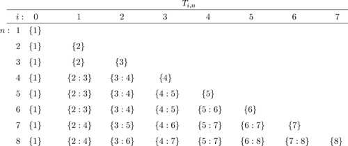
As stated earlier, $\mathcal{T}$ can be visualized as a triangular array of sets – see Figure 1. This was computed by brute force. For instance, the last row corresponds to n = 8 and was computed by generating all $2^7$ sequences $f\in {\mathcal{S}}_8$, finding the sequences q corresponding to each and noting the different values of $q(8){|}_{f(8)=i}$, for $0\le i\le 7$. As an example, the fourth row of Figure 1 implies that, for instance,

• If $f(4)=0$, $q(4)$ can only be 1, that is, $T_{0,4}=\{1\}$. This is obvious since the sequence f, $f\in {\mathcal{S}}_4$, can only be $(0,0,0,0)$. See Lemma 3.2.

• Now suppose that $f(4)=1$. In this case, the allowed sequences f are $(0,0,0,1)$, $(0,0,1,1)$ and $(0,1,1,1)$. Using (3(3) $q(n)=q(n-q(n-1))+f(n)\mathrm{with}q(1)=1,$(3) ) to compute $q(4)$ in each case, we find that the first two give $q(4)=2$ and the third one, $q(4)=3$. Thus, $T_{1,4}=\{2,3\}$ (cf. $U_{1,4}=\{2,3,4\}$).

Figure 1. The first eight rows of the triangular array of sets $\mathcal{T}$. Here, i and n index the sets horizontally and vertically respectively, with $i=0,\dots ,n-1$. The set of consecutive integers $k,\dots ,l$ is written $\{k:l\}$ and as $\{k\}$ when l = k.

4. Examples of sequences q that are slow

In Lemma 3.2, we gave the examples $f(n)=0$ and $f(n)=n-1$, both of which lead to sequences q that are slow. We are aware of three other examples, which we now present.

The first example is given in

Lemma 4.1

$\mathrm{If}f(n)=\lfloor \frac{n+2}{4}\rfloor \mathrm{then}q(n)=\lfloor \frac{n+2}{2}\rfloor .$

Proof.

Let $\tilde{q}(x)=\frac{x}{2}+\frac{3+\cos \mathrm{\pi x}}{4}$for $x\in \mathbb{R}$. Then it can easily be verified that $\tilde{q}(n)=\lfloor \frac{n+2}{2}\rfloor$ for $n\in \mathbb{N}$. Furthermore, direct calculation gives $\tilde{q}(x)-\tilde{q}(x-\tilde{q}(x-1))=\frac{1}{8}(2x+1+\cos \mathrm{\pi x})-\frac{1}{4}\sin \left(\frac{\pi (2x+1+\cos \mathrm{\pi x})}{4}\right):=\tilde{f}(x).$Finally, it is straightforward to check that, for $n\in \mathbb{N}$, $\tilde{f}(n)=\lfloor \frac{n+2}{4}\rfloor$ and this proves the lemma.

Remark 4.2

We have proved more here, viz. that $\tilde{q}(x)$, $\tilde{f}(x)$ as given above obey $\tilde{q}(x)=\tilde{q}(x-\tilde{q}(x-1))+\tilde{f}(x)$ for all $x\in \mathbb{R}$: a continuous solution to (3(3) $q(n)=q(n-q(n-1))+f(n)\mathrm{with}q(1)=1,$(3) ). The same is true of $f_0(x)=0$, which implies that $q_0(x)=1$, and $f_1(x)=x-1$, which implies that $q_1(x)=x$, both for $x\in \mathbb{R}$ – an extension of Lemma 3.2.

For the second example, define (8) $\delta (n):=\{\begin{array}{ll}1,& n=0\\ 0,& \mathrm{otherwise},\end{array}$(8) for $n\in \mathbb{Z}$. Another instance of a slow sequence q is found when $f(n)=1-\delta (n-1)$: in fact, $Q(1-\delta (n-1))=1,2,2,3,3,3,4,\dots$, where each positive integer k occurs k times. This sequence can also be written $\mathrm{For}k\in \mathbb{N},q(n)=k\mathrm{for}h(k)\le n\le h(k+1)-1,\mathrm{with}h(k):=\frac{k^2-k+2}{2}.$We summarize these observations in the following lemma:

Lemma 4.3

Let $f(n)=1-\delta (n-1)=(0,1,1,\dots )$. Then $q(n)=(1,2,2,3,3,3,4,\dots )$, where each positive integer appears in turn, with integer k occurring k times in succession. That is, $q(n)=k\mathrm{for}h(k)\le n\le h(k+1)-1,$where $k\in \mathbb{N}$ and $h(k)=\frac{k^2-k+2}{2}$.

This sequence [8] is a special case of a generalized Golomb triangular recursion [4]. A proof of Lemma 4.3 by S.W. Golomb can be found in the ‘Links’ section of [8].

Remark 4.4

This result can also be written as $f(n)=1-\delta (n-1)\Rightarrow q(n)=\lfloor \frac{1}{2}+\sqrt{2n-\frac{7}{4}}\rfloor =:w(n),$as can be easily shown by considering $\sqrt{2h(k)-7/4}=k-1/2$ for $k\in \mathbb{N}$. However, we lack a direct proof of Lemma 4.3 starting from this expression.

Remark 4.5

This result relates immediately to the fact that $T_{1,n}⊊U_{1,n}$: we have explicitly constructed $T_{1,n}=\{2:w(n)\}$ above, from which it is clear that $T_{1,n}⊊U_{1,n}$ for n>2. See the second column from the left in Figure 1.

The third example of a slow sequence q is especially interesting and involves γ, the reciprocal of the golden ratio:

Theorem 4.6

Let $\gamma :=\frac{\sqrt{5}-1}{2}$, so that ${\gamma }^2+\gamma -1=0$. Then $q(n)=1+\lfloor \gamma (n-1)\rfloor$ obeys (3(3) $q(n)=q(n-q(n-1))+f(n)\mathrm{with}q(1)=1,$(3) ) with $f(n)=\lfloor {\gamma }^{2}n\rfloor$.

Since $\gamma \approx 0.618<1$, clearly $q(n)$ as defined here is slow, and, furthermore, $q(1)=1$.

In the course of the proof of the theorem, we need a few small results:

1. ¹${\gamma }^2+\gamma =1$, which implies that $2{\gamma }^2+3\gamma =2+\gamma$, ${\gamma }^{-1}=1+\gamma$, ${\gamma }^2(\gamma +2)=1$.

2. $x=\lfloor x\rfloor +\{x\}$, $x\in \mathbb{R}$, where $\{x\}$ is the fractional part of x

3. $\lfloor -x\rfloor =-\lfloor x\rfloor -1$, $x\notin \mathbb{Z}$

4. $\lfloor m+x\rfloor =m+\lfloor x\rfloor$ for $m\in \mathbb{N}$

5. $\{{\gamma }^{2}n\}=1-\{\mathrm{\gamma n}\}$.

Item (i) comes from the given definition of γ and (ii)–(iv) are from the definition of the floor function. For (v), start from (ii) with $x={\gamma }^{2}n$, which gives $\{{\gamma }^{2}n\}={\gamma }^{2}n-\lfloor {\gamma }^{2}n\rfloor$. Now use (i) to replace ${\gamma }^2$ with $1-\gamma$, giving $\{{\gamma }^{2}n\}=n-\mathrm{\gamma n}-\lfloor n-\mathrm{\gamma n}\rfloor =-\mathrm{\gamma n}-\lfloor -\mathrm{\gamma n}\rfloor$, where (iv) has been used. Then (iii) gives $\{{\gamma }^{2}n\}=-\mathrm{\gamma n}+\lfloor \mathrm{\gamma n}\rfloor +1=1-\{\mathrm{\gamma n}\}$, using (ii).

Proof of Theorem 4.6

We first show that the theorem is equivalent to identity (9(9) $\theta (n):=\lfloor \gamma +\gamma \lfloor {\gamma }^2(n-1)\rfloor \rfloor +\lfloor {\gamma }^{2}n\rfloor +\lfloor {\gamma }^2(n+1)\rfloor =n-1\mathrm{for}n\in \mathbb{N}.$(9) ) below, then we prove the identity itself.

Starting from $q(n)=1+\lfloor \gamma (n-1)\rfloor$, clearly $q(1)=1$. It is convenient to shift n by 1, giving $q(n+1)=1+\lfloor \mathrm{\gamma n}\rfloor$, which we will show obeys (3(3) $q(n)=q(n-q(n-1))+f(n)\mathrm{with}q(1)=1,$(3) ) for $n\in \mathbb{N}$. When this is substituted in $q(n+1)-q(n+1-q(n))$ we have $q(n+1)-q(n+1-q(n))=\lfloor \mathrm{\gamma n}\rfloor -\lfloor \gamma (n-1)-\gamma \lfloor \gamma (n-1)\rfloor \rfloor .$Now, using (i), (iii) and (iv), we find that $q(n+1)-q(n+1-q(n))=n-1-\lfloor {\gamma }^{2}n\rfloor -\lfloor \gamma +\gamma \lfloor {\gamma }^2(n-1)\rfloor \rfloor .$Hence, Theorem 4.6 holds if the right-hand side of the above expression is equal to $f(n+1)=\lfloor {\gamma }^2(n+1)\rfloor$ for $n\in \mathbb{N}$, that is, if (9) $\theta (n):=\lfloor \gamma +\gamma \lfloor {\gamma }^2(n-1)\rfloor \rfloor +\lfloor {\gamma }^{2}n\rfloor +\lfloor {\gamma }^2(n+1)\rfloor =n-1\mathrm{for}n\in \mathbb{N}.$(9) To prove (9(9) $\theta (n):=\lfloor \gamma +\gamma \lfloor {\gamma }^2(n-1)\rfloor \rfloor +\lfloor {\gamma }^{2}n\rfloor +\lfloor {\gamma }^2(n+1)\rfloor =n-1\mathrm{for}n\in \mathbb{N}.$(9) ), we consider separately three cases which are demarcated according to $\text{Case A:}\{{\gamma }^{2}n\}\in (0,{\gamma }^2);\text{Case B:}\{{\gamma }^{2}n\}\in ({\gamma }^2,\gamma );\text{Case C:}\{{\gamma }^{2}n\}\in (\gamma ,1).$For n>1, these intervals are all open because γ and ${\gamma }^2=(3-\sqrt{5})/2$ are irrational. Hence, we first dispose of the case n = 1, where we find $\theta (1)=\lfloor \gamma +0\rfloor +\lfloor {\gamma }^2\rfloor +\lfloor 2{\gamma }^2\rfloor =0=n-1,$since ${\gamma }^2<1/2$.

We assume that $n\ge 2$ throughout the rest of this proof. Proving cases A–C for $n\ge 2$ amounts primarily to rearranging $\theta (n)$ into a first-degree polynomial in n, plus the floor of a bounded function of n.

Case A. Note that $\{{\gamma }^{2}n\}\in (0,{\gamma }^2)$ implies that $\lfloor {\gamma }^2(n-1)\rfloor =\lfloor {\gamma }^2(n)\rfloor -1$ and $\lfloor {\gamma }^2(n+1)\rfloor =\lfloor {\gamma }^2(n)\rfloor$. Thus, in case A we have $\theta (n)=\lfloor \gamma \lfloor {\gamma }^{2}n\rfloor \rfloor +2\lfloor {\gamma }^{2}n\rfloor =:{\theta }_A(n).$Consider the first term in ${\theta }_A(n)$: $\lfloor \gamma \lfloor {\gamma }^{2}n\rfloor \rfloor =\lfloor \gamma \lfloor (1-\gamma )n\rfloor \rfloor =\lfloor \mathrm{\gamma n}-\gamma (\lfloor \mathrm{\gamma n}\rfloor +1)\rfloor =\lfloor \mathrm{\gamma n}-\gamma (\mathrm{\gamma n}-\{\mathrm{\gamma n}\}+1)\rfloor ,$where we have used (i), (iv), (iii) and then (ii). Replacing the first $\mathrm{\gamma n}$ with $(1-{\gamma }^2)n$, we get $\lfloor \gamma \lfloor {\gamma }^{2}n\rfloor \rfloor =n+\lfloor -2{\gamma }^{2}n+\gamma \{\mathrm{\gamma n}\}-\gamma \rfloor =n-1-\lfloor 2{\gamma }^{2}n-\gamma \{\mathrm{\gamma n}\}+\gamma \rfloor ,$using (iii). We can now use (ii) and (v) to obtain $\lfloor \gamma \lfloor {\gamma }^{2}n\rfloor \rfloor =$ $n-1-\lfloor 2(\lfloor {\gamma }^{2}n\rfloor +\{{\gamma }^{2}n\})+\gamma (1-\{\mathrm{\gamma n}\})\rfloor =n-1-\lfloor 2(\lfloor {\gamma }^{2}n\rfloor +\{{\gamma }^{2}n\})+\gamma \{{\gamma }^{2}n\}\rfloor .$Hence, using (iv), ${\theta }_A(n)=n-1-\lfloor 2(\lfloor {\gamma }^{2}n\rfloor +\{{\gamma }^{2}n\})+\gamma \{{\gamma }^{2}n\}\rfloor +2\lfloor {\gamma }^{2}n\rfloor =n-1-\lfloor (\gamma +2)\{{\gamma }^{2}n\}\rfloor ,$and ${\theta }_A(n)$ is now in the required form.

Since $0<\{{\gamma }^{2}n\}<{\gamma }^2$, we have, in case A, $0<(\gamma +2)\{{\gamma }^{2}n\}<{\gamma }^2(\gamma +2)=1$, using (i), and so $\lfloor (\gamma +2)\{{\gamma }^{2}n\}\rfloor =0$. Therefore, ${\theta }_A(n)=n-1$.

Case B. For case B, we have ${\gamma }^2<\{{\gamma }^{2}n\}<\gamma =1-{\gamma }^2$ and this implies that $\lfloor {\gamma }^2(n-1)\rfloor =\lfloor {\gamma }^{2}n\rfloor =\lfloor {\gamma }^2(n+1)\rfloor$. Hence, in case B $\theta (n)=\lfloor \gamma +\gamma \lfloor {\gamma }^{2}n\rfloor \rfloor +2\lfloor {\gamma }^{2}n\rfloor =:{\theta }_B(n).$Since $2\lfloor {\gamma }^{2}n\rfloor$ is an integer, we immediately have ${\theta }_B(n)=\lfloor \gamma +(\gamma +2)\lfloor {\gamma }^{2}n\rfloor \rfloor$. Now, $(\gamma +2)\lfloor {\gamma }^{2}n\rfloor =(\gamma +2)({\gamma }^{2}n-\{{\gamma }^{2}n\})=n-(\gamma +2)\{{\gamma }^{2}n\},$by (ii) and (i). Hence, (10) ${\theta }_B(n)=n+\lfloor \gamma -(\gamma +2)\{{\gamma }^{2}n\}\rfloor =n-1-\lfloor (\gamma +2)\{{\gamma }^{2}n\}-\gamma \rfloor ,$(10) using (iii). Now, by the definition of case B, ${\gamma }^2(\gamma +2)<(\gamma +2)\{{\gamma }^{2}n\}<\gamma (\gamma +2)\mathrm{or}1<(\gamma +2)\{{\gamma }^{2}n\}<\gamma +1.$Hence, $\lfloor (\gamma +2)\{{\gamma }^{2}n\}-\gamma \rfloor =0$ and ${\theta }_B(n)=n-1$.

Case C. Case C is similar to case B. We now have $\gamma <\{{\gamma }^{2}n\}<1$, giving $\lfloor {\gamma }^2(n-1)\rfloor =\lfloor {\gamma }^{2}n\rfloor$ but $\lfloor {\gamma }^2(n+1)\rfloor =\lfloor {\gamma }^{2}n\rfloor +1$. Hence, in case C $\theta (n)=\lfloor \gamma +\gamma \lfloor {\gamma }^{2}n\rfloor \rfloor +2\lfloor {\gamma }^{2}n\rfloor +1=:{\theta }_C(n).$From the definition of ${\theta }_B(n)$, we see immediately that ${\theta }_C(n)={\theta }_B(n)+1$ and so, from (10(10) ${\theta }_B(n)=n+\lfloor \gamma -(\gamma +2)\{{\gamma }^{2}n\}\rfloor =n-1-\lfloor (\gamma +2)\{{\gamma }^{2}n\}-\gamma \rfloor ,$(10) ), we have ${\theta }_C(n)=n-\lfloor (\gamma +2)\{{\gamma }^{2}n\}-\gamma \rfloor$. Hence, for case C, $\gamma (\gamma +2)<(\gamma +2)\{{\gamma }^{2}n\}<(\gamma +2)\mathrm{or}1<(\gamma +2)\{{\gamma }^{2}n\}-\gamma <2.$Therefore, $\lfloor (\gamma +2)\{{\gamma }^{2}n\}-\gamma \rfloor =1$ and so ${\theta }_C(n)=n-1$, concluding the proof of the theorem.

5. Heuristic and experimental results

In this section we present heuristic plausibility arguments to give simple descriptions of the behavior of q for certain sequences f. As we shall see, computation suggests that the actual behavior of q follows our predictions closely. We consider three types of sequence f.

5.1. $\mathit{f}\mathbf{(}\mathit{n}\mathbf{)}\mathbf{=}\mathbf{\lfloor }\mathit{\alpha n}\mathbf{\rfloor }$, $\mathit{\alpha }\mathbf{\in }\mathbf{(}\mathbf{0}\mathbf{,}\mathbf{1}\mathbf{)}$

The following lemma summarizes what we can say about the behavior of $q(n)$ in this case.

Lemma 5.1

Let $f(n)=\lfloor \mathrm{\alpha n}\rfloor$ with $\alpha \in (0,1)$. Assume that $q(n)=\mathrm{an}+ϵ(n)$, where $a\in (0,1)$ is a constant, and that $\underset{n\to \mathrm{\infty }}{lim}ϵ(n)/n=0$. Then $a=\sqrt{\alpha }$.

Proof.

Substituting $q(n)=\mathrm{an}+ϵ(n)$ in Equation (3(3) $q(n)=q(n-q(n-1))+f(n)\mathrm{with}q(1)=1,$(3) ) gives $\mathrm{an}+ϵ(n)=a(n-a(n-1)-ϵ(n-1))+ϵ(n-a(n-1)-ϵ(n-1))+\mathrm{\alpha n}-\left\{\mathrm{\alpha n}\right\},$and solving for $ϵ(n)$ gives $ϵ(n)=-a^2(n-1)-\mathrm{aϵ}(n-1)+ϵ(n-a(n-1)-ϵ(n-1))+\mathrm{\alpha n}-\left\{\mathrm{\alpha n}\right\}.$Dividing both sides by n and letting $n\to \mathrm{\infty }$ gives $a^2=\alpha$ and so (11) $q(n)=\sqrt{\alpha }n+o(n).$(11)

This turns out to be a good approximation. For an example, see Figure 3, which shows $q(n)-n/\sqrt{2}$ when $f(n)=\lfloor n/2\rfloor$. For $n\le 160000$, we find from the data used to produce this figure that $|q(n)-n/\sqrt{2}|<75.5$.

Theorem 4.6 is a particular case of Equation (11(11) $q(n)=\sqrt{\alpha }n+o(n).$(11) ) with $\alpha ={\gamma }^2$.

5.2. $\mathit{f}\mathbf{(}\mathit{n}\mathbf{)}\mathbf{=}\mathit{a}\mathbf{for}\mathit{n}\mathbf{>}{\mathit{n}}^{\mathbf{\prime }}$

The case $f(n)$ tends to a constant $a\in \mathbb{N}$ as $n\to \mathrm{\infty }$ is interesting, and is a special case of a nested recursion studied in [10]. We argue by proposing the ansatz $q(x)=\sqrt{2\mathrm{ax}}-b$, $x\in \mathbb{R}$, and then deducing the $f(x)$ that this implies. Starting from the asymptotic expansion: $f(x)=q(x)-q(x-q(x-1))\sim a+\frac{\sqrt{2a}(a-2b)}{4\sqrt{x}}+\frac{a(a-2b-2)}{4x}+O\left(x^{-\frac{3}{2}}\right),$we let $b=a/2$ in order to eliminate the second term. This gives $f(x)\sim a-\frac{a}{2x}+O\left(x^{-\frac{3}{2}}\right).$This short calculation suggests that, for $a,n\in \mathbb{N}$, (12) $f(n)=a-\lfloor {\delta }_1(n)\rfloor ⟹q(n)=\sqrt{2\mathrm{an}}-a/2+{\delta }_2(n),$(12) where ${\delta }_1(1)=a$ and ${\delta }_i(n)\to 0$ as $n\to \mathrm{\infty }$, i = 1, 2.

This appears to work surprisingly well – see Figure 2, which compares q when $f(n)=\lfloor 5-5/\sqrt{n}\rfloor )$, so that $\underset{n\to \mathrm{\infty }}{lim}f(n)=4$, with $s(n):=\sqrt{8n}-2$ for $n=1,\dots ,{10}^5$. Over this range, we find that $|q(n)-s(n)|<2$.

Figure 2. Plot of $q(n)$, black dots, for $f(n)=\lfloor 5-5/\sqrt{n}\rfloor$, so that $f(n)\to 4$ as $n\to \mathrm{\infty }$. According to the argument in Section 5.2, we expect that $q(n)\sim \sqrt{8n}-2:=s(n)$, this curve being plotted as a continuous black line. The approximation appears to hold remarkably well, the two plots being almost exactly superimposed. Inset: enlargement of the region $75000\le n\le 80000$.

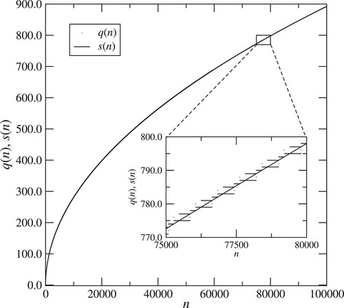
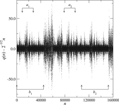
Figure 3. Plot of $q(n)-n/\sqrt{2}$ for $n=1,\dots ,160000$, with $f(n)=\lfloor \frac{n}{2}\rfloor$. Two pairs of self-similar regions $a_1,a_2$ and $b_1,b_2$ are shown – see text.

Other examples were tried: $f(n)=\lfloor a-\mathrm{aexp}(-\mathrm{bn})\rfloor$, $f(n)=\lfloor a-a/n^b\rfloor$ and $f(n)=\lfloor \mathrm{an}\rfloor$ if $n<n_0$ and $\lfloor a{n}_0\rfloor$ otherwise. In all cases, a, b were chosen so as to ensure that $f(n)$ had property ${\mathrm{S}}_0$, and every time, (12(12) $f(n)=a-\lfloor {\delta }_1(n)\rfloor ⟹q(n)=\sqrt{2\mathrm{an}}-a/2+{\delta }_2(n),$(12) ) gave an excellent approximation to $q(n)$: in these cases at least, it is the asymptotic behavior of $f(n)$ that determines the asymptotic behavior of $q(n)$.

5.3. $\mathit{f}\mathbf{(}\mathit{n}\mathbf{)}\mathbf{=}\mathbf{\lfloor }{\mathit{c}}_{\mathbf{1}}{\mathit{n}}^{{\mathit{p}}_{\mathbf{1}}}\mathbf{+}{\mathit{c}}_{\mathbf{2}}{\mathit{n}}^{{\mathit{p}}_{\mathbf{2}}}\mathbf{+}\mathbf{\dots }\mathbf{\rfloor }$ with ${\mathit{p}}_{\mathit{i}}\mathbf{\in }\mathbf{(}\mathbf{0}\mathbf{,}\mathbf{1}\mathbf{)}$

Arguing in reverse as in the previous case, we can obtain useful approximations to $q(n)$ when $f(n)$ is the sum of fractional powers of n, at least in certain special cases. We use the ansatz $q(x)=a{x}^p+b$ and calculate the asymptotic expansion for $\begin{array}{rl}f(x)& =q(x)-q(x-q(x-1))\sim \mathrm{ap}[b{x}^{p-1}+\frac{b^2(1-p)}{2}{x}^{p-2}+\dots \\ & +a{x}^{2p-1}+a(b(1-p)-p)x^{2p-2}+\dots \\ & +\frac{a^2(1-p)}{2}{x}^{3p-2}+\frac{a^2(1-p)(b(2-p)-2p)}{2}{x}^{3p-3}+\dots ].\end{array}$Note that the powers of x here are p−i, $i\in \mathbb{N}$ and ip−j, $i\ge 2$, $j\ge i-1$. We cannot order the powers of x unless a value of p is specified. Letting, for example, a = 1, $b=1/2$ and $p=3/4$, we have $f(x)=3x^{\frac{1}{2}}/4+3x^{\frac{1}{4}}/32+5/128+O(x^{-\frac{1}{4}})$ and $q(x)=x^{\frac{3}{4}}+1/2$. Then, with $f(n)=\lfloor 3n^{\frac{1}{2}}/4+3n^{\frac{1}{4}}/32+5/128\rfloor$, which has property ${\mathrm{S}}_0$, we generate $q(n)$ via (3(3) $q(n)=q(n-q(n-1))+f(n)\mathrm{with}q(1)=1,$(3) ) and compare this with our approximation $q^{\prime }(n):=n^{\frac{3}{4}}+1/2$. The agreement is good, with $-21\le q(n)-q^{\prime }(n)\le 3$ for $1\le n\le N=160000$, where $q(N)=7990$.

5.4. Dynamics

We close this section with some figures illustrating examples of the dynamics of q for particular sequences f.

An interesting case is $q=Q(\lfloor n/2\rfloor )$, shown in Figure 3. This shows the de-trended sequence $q(n)-n/\sqrt{2}$ – see (11(11) $q(n)=\sqrt{\alpha }n+o(n).$(11) ) – for $1\le n\le 160000$. At first sight, no obvious patterns appear in the plot, but in fact there are several regions of exact self-similarity, even in this limited range of n. Specifically, among others, we observe

• $q(i+69568)-q(i)=49192\mathrm{for}i\in \{9235:27465\}$ (regions $a_1,a_2$); and

• $q(i+107616)-q(i)=76096\mathrm{for}i\in \{91:44577\}$ (regions $b_1,b_2$).

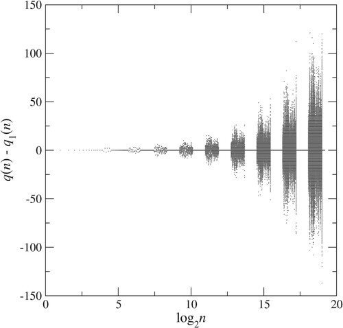
Our final figure gives an intuitive idea of what happens if we make a small perturbation. It is tempting to describe the behavior of many of the sequences $Q(f)$ as ‘chaotic’. However, since (3(3) $q(n)=q(n-q(n-1))+f(n)\mathrm{with}q(1)=1,$(3) ) is discrete in time and space, there is no sense in which the system can be infinitesimally perturbed; perhaps the best we can do is to compute sequences q, $q_1$, where $q_1$ is computed identically to q – using (3(3) $q(n)=q(n-q(n-1))+f(n)\mathrm{with}q(1)=1,$(3) ) in the usual way – except that we artificially adjust a single term, $q(n_1)$ say, for some small integer $n_1$. The result of such a computation, with $q=Q(\lfloor n/2\rfloor )$, $q_1=Q(\lfloor n/2\rfloor +\delta (n-16))$, so that $q_1(16)=1+q(16)$, is shown in Figure 4. This figure is a plot of the difference $q(n)-q_1(n)$ versus ${\log }_2(n)$, the scaling bringing out the approximate periodicity visible on a logarithmic scale. We see regions where $q(n)-q_1(n)=0$ exactly, interspersed with regions where this difference is far from zero: the memory of the perturbation seems to persist indefinitely.

Figure 4. Plot of the difference of $q(n)=Q(\lfloor n/2\rfloor )$ and $q_1(n)=Q(\lfloor n/2\rfloor +\delta (n-16))$. The idea is that $q_1(n)$ is a slightly perturbed version of $q(n)$. The effect of the perturbation persists, at least until $n=2^{19}$.

6. Conclusions and further work

We have investigated the problem of the conditions on an integer sequence $f(n)$, $n\in \mathbb{N}$, with $f(1)=0$, such that the sequence $q(n)$, with $q(1)=1$, computed from $q(n)=q(n-q(n-1))+f(n)$, exists. We think of the sequence q as a solution to this difference equation. We have proved that if $f(n+1)-f(n)\in \{0,1\}$, $n\ge 1$, then the solution q exists, the existence of q being exactly equivalent to the inequality $1\le q(n)\le n$ holding for all $n\in \mathbb{N}$.

We have defined $\mathcal{S}$ as the set of semi-infinite slow sequences (that is, sequences with differences between successive terms equal to 0 or 1)². In Lemma 2.1 examples were given of sequences $f\notin \mathcal{S}$ but for which q nonetheless exists – the condition that f be slow is sufficient but not necessary – and this suggests that we define a second set of semi-infinite integer sequences, $\mathcal{F}$, which is the set of all sequences f with $f(1)=0$ such that the corresponding sequence q exists. Clearly, $\mathcal{S}⊊\mathcal{F}$.

It would be fruitful to investigate the structure of $\mathcal{F}$ further. The question naturally arises as to whether the proof of Theorem 1.3 could be extended to include more sequences f. A better characterization of $\mathcal{F}$ might be a useful step on the way to settling the question of the existence of the Hofstadter sequence, this problem being the original motivation for our work. In fact, the question would have been settled by Theorem 1.3, were the sequence $c(n):=q_h(n-q_h(n-2))$, with $q_h$ defined by (1(1) $q_h(n)=q_h(n-q_h(n-1))+q_h(n-q_h(n-2))\mathrm{with}{q}_h(1)=q_h(2)=1.$(1) ), to be slow. It is not – in fact $c=(1,2,2,2,3,3,3,3,3,4,5,4,5,\dots )$.

Solutions arising from $f\in \mathcal{S}$ typically appear to display non-trivial dynamics: in particular, they are generally aperiodic and display no obvious patterns. For some special sequences f, for instance $f(n)=\lfloor \mathrm{\alpha n}\rfloor$ with $\alpha \in [0,1)$, the average behavior appears to be well-defined, however, and we give a heuristic argument for this.

Less typical seem to be sequences $f\in \mathcal{S}$ for which the corresponding solution is also monotonic, and we construct exact solutions in the cases of which we are aware.

Both from the point of view of the existence of solutions and from the study of their dynamics, the difference Equation (3(3) $q(n)=q(n-q(n-1))+f(n)\mathrm{with}q(1)=1,$(3) ) appears to be an interesting subject for further study, even in its own right.

Acknowledgments

The Authors would like to acknowledge helfpul discussions with Dr Peter Gallagher and the valuable comments of the anonymous referees of this journal.

Disclosure statement

No potential conflict of interest was reported by the author(s).

Notes

1 (i), (ii) etc would be clearer labels than i, ii

2 It would be useful to add  "and with first term equal to zero" here, i for consistency with the original definition of S.

References

- B. Balamohan, A. Kuznetsov, and S. Tanny, On the behavior of a variant of Hofstadter's Q-sequence, J. Integer Seq. 10 (2007), Article 07.7.1.
- N. Fox, Quasipolynomial solutions to the Hofstadter Q-recurrence, Integers 16 (2016), paper A68, 6 pp.
- D.R. Hofstadter, Gödel, Escher, Bach: An Eternal Golden Braid, Basic Books, Springer, New York, 1979. ISBN 0-465-026850.
- A. Isgur, V. Kuznetsov, and S.M. Tanny, A combinatorial approach for solving certain nested recursions with non-slow solutions, J. Differ. Equ. Appl. 19(4) (2013), pp. 604–615. https://doi.org/10.1080/10236198.2012.662967.
- OEIS Foundation Inc., Entry A005185 in the On-Line Encyclopedia of Integer Sequences, 2024; Available at https://oeis.org/A005185 (in particular the reference to a computation by M. Eric Carr (2 July 2023)).
- OEIS Foundation Inc., Entry A006949 in the On-Line Encyclopedia of Integer Sequences, 2024; Available at https://oeis.org/A006949.
- OEIS Foundation Inc., Entry A063882 in the On-Line Encyclopedia of Integer Sequences, 2024; Available at https://oeis.org/A063882.
- OEIS Foundation Inc., Entry A002024 in the On-Line Encyclopedia of Integer Sequences, 2024; Available at https://oeis.org/A002024.
- K. Pinn, Order and chaos in Hofstadter's Q(n) sequence, Complexity 4(3) (1999), pp. 41–46.
- M. Sunohara and S.M. Tanny, On the solution space of the Golomb recursion, J. Differ. Equ. Appl. 24(8) (2018), pp. 1273–1294. https://doi.org/10.1080/10236198.2018.1471471.
- S.M. Tanny, A well-behaved cousin of the Hofstadter sequence, Discrete Math. 105(1–3) (1992), pp. 227–239.