The Impact of Military Expenditures on Economic Growth: A New Instrumental Variables Approach

ABSTRACT

Endogeneity problems have plagued efforts to estimate the impact of military expenditures on economic growth. This paper addresses this problem with two instruments for military expenditures: the value of arms imports during periods of peace and the number of neighboring states suffering interstate violence. While positively correlated with military expenditures, the value of arms imports is unlikely to be determined by economic growth because of the time lag which exists, which in many cases runs into several years, between the placement of purchase orders for these arms and their delivery. The number of neighboring states suffering interstate violence captures regional ‘political uncertainty’, which spurs military spending without capturing the actual scale of domestic political violence which may directly affect economic growth. Several diagnostic tests show that both these instruments are highly correlated with military expenditures and fulfill overidentification restrictions. The results from empirical analyses of panel data on 133 countries during the 1960-2012 period indicate that an increase in military expenditure/GDP of 1 percentage point reduces economic growth by 1.10 percentage points. These results are robust to the application of 2SLS, LIML, and GMM estimators.

KEYWORDS:

• Military expenditures
• economic growth
• instrumental variable approach
• 2SLS
• GMM

JEL CLASFFICATION:

• 040
• 047
• 011
• C26
• C33

Introduction

This study examines the impact of military expenditures on economic growth and proposes a new identification strategy for tackling the endogeneity of military expenditures in the growth model. The empirical findings on whether military expenditures stimulate (through channels such as increasing employment opportunities, transfer of military technology to civilian industries etc.) or retard economic growth (for instance by crowding out productive investment) are mixed (Dunne and Tian 2013). This heterogeneity in findings is mainly attributed to differences in samples and model specifications (Aziz and Asadullah 2017) but more importantly to the endogeneity of military expenditures variable in the growth model (d’Agostino, Dunne, and Pieroni 2019; Smith 2017). The potential sources of this endogeneity problem are manifold. For instance, economic growth can exert a reverse causal impact on military expenditures as higher growth makes additional resources available for defense build-up. Also, as discussed in detail in the Empirical Strategy section, both economic growth and military expenditure variables are likely to be affected by common unobserved factors (d’Agostino, Dunne, and Pieroni 2019). As a result, the estimates drawn from the growth models which do not account for the endogeneity of military expenditures can be biased.

This paper proposes two new instruments for the military expenditures variable in the growth model: arms imports during peace time (when yearly battle-related deaths are below 25) and the number of neighboring states suffering interstate violence. Illustrated in detail in the section Empirical Strategy, the effects of these two instruments on economic growth are likely to channel through their impact on the military expenditures variable. The results from several diagnostic tests provide supporting evidence that both these instruments are highly correlated with the military expenditures variable and satisfy overidentification restrictions.

The regression analysis exploits panel data on 133 countries covering the time period of 1960-2012. The results from IV regressions suggest that a 1 percentage point increase in military expenditures as a percentage of GDP leads to approximately a 1.10 percentage points reduction in economic growth. This estimate of −1.10 is approximately 4 times larger in size than the estimate of −0.281 obtained from a fixed effect model that includes military expenditures as an exogenous variable. The statistically significant negative effect of military expenditures on economic growth is consistently observed in samples of developing, conflict-affected and below than average human rights performers countries.

The empirical literature on the impact of military spending on economic growth abounds. Several literature reviews already exist which provide insightful overviews of the major trends in the findings from the studies published over the past four decades (Dunne, Smith, and Willenbockel 2005; Dunne and Tian 2013; Ram 1995; Smaldone 2006). Therefore, this study restricts itself to a very brief discussion of the literature. Theoretical and empirical works of Clive Trebilcock (1969, 1973) and Emile Benoit (1973, 1978) during the 1970s initiated a serious debate on the utility of the defense sector for economic development. Their work was followed by a plethora of studies that employed econometric methodologies to analyze case studies (Ahmed et al. 2020; Antonakis 1997; Chan 1988; DeRouen 2000; Phiri 2019), and n sample studies (Aizenman and Glick 2006; Aziz and Asadullah 2017; Blomberg 1996; Cappelen and Bjerkholt 1984; Dunne and Mohammad 1995; Karadam, Yildirim, and Ocal 2016; Kollias, Mylonidis, and Paleologou 2007; Landau 1996; Stroup and Heckelman 2001; Yakovlev 2007). Table A1 in Appendix I provides a summary of the main findings from these studies.

While empirical findings drawn mainly from the regression analyses have long been mixed, however, potentially due to the increasing availability of data in the post-Cold war period, a consistent pattern is unfolding in the findings which indicate a negative impact of military expenditures on growth (d’Agostino, Dunne, and Pieroni 2019). Dunne and Uye (2009) observed in a survey of 103 studies that only 20 studies showed a positive impact of military expenditure on growth/development. The negative impact was observed in 37 studies, whereas in the remaining 43 studies, the results were inconclusive.

However, the endogeneity problem remains a key concern in drawing inferences about the causal impact of military expenditures on economic growth. The challenge is to identify instrument(s) which cause exogenous variations in military expenditures but not in the economic growth variable (d’Agostino, Dunne, and Pieroni 2019; Smith 2017). While some studies, such as Chang, Huang, and Yang (2011), exploited pre-determined lag values of military expenditures as instruments and employed Arellano and Bond (1991) estimator for estimation; to the best of the author’s knowledge, d’Agostino, Dunne, and Pieroni (2019) is the only study which employed excluded instrument obtained from outside of the data as an instrument for military expenditures. d’Agostino, Dunne, and Pieroni (2019) employ a dummy variable that captures the transition from unrest to turmoil as an instrument for military expenditures. The threshold level for turmoil is set at a level where the number of organized violence¹ events exceeds the mode of its distribution. The relevance of the instrument is based on the premise that it reflects the ‘political environment’ that a country faces without capturing the destruction produced by the related activities (d’Agostino, Dunne, and Pieroni 2019). The results from their empirical analyses of 109 non-high-income countries, covering the period of 1988-2012, suggest that the negative impact of military expenditure on economic growth is larger than the one indicated by the estimate from the OLS model. The size of the estimate increases from −0.629 in the OLS model to −2.791 in the IV model. The empirical strategy in d’Agostino, Dunne, and Pieroni (2019) is certainly a valuable addition to the existing literature. However, their econometric model is ‘just identified’ which implies that while the correlation of the instrument with military expenditures can be examined, whether the instrument is uncorrelated with the error term, i.e. $corr\left(Z_{it},{\mu }_{it}\right)=0$, remains untested.

As a step forward, this study suggests two new instruments which allow testing of overidentification restrictions. The next section outlines the empirical strategy and provides arguments in favor of the plausibility of these two instruments.

Empirical Strategy

The study employs regression analysis to estimate the impact of military expenditures on economic growth. However, as discussed in the previous section, the issue of endogeneity remains a main concern.

Consider the following fixed effect model,

(1) $GR={\beta }_0+{\beta }_{1}ME/GD{P}_{it}+{\beta }_2{X}_{it}+{\delta }_i+{\mu }_{it}$(1)

Where GR= Growth Rate, ME/GDP= Military expenditure/GDP, X= vector of control variables, $\delta$ =country-level fixed effects and $\mu$= error term.

The coefficient of interest in this model is ${\beta }_1$. This coefficient can be biased for two reasons. First, there is a possible reverse causal impact of economic growth on military expenditures (d’Agostino, Dunne, and Pieroni 2019).² Second, both economic growth and military expenditure variables are likely to be affected by unobserved common factors. Since it is not possible to quantify all such factors hence, they are included in the error term. While to some extent, country-level fixed effects $\delta$, can capture time-invariant unobservables, such as geography, other potential sources of influences on military expenditures and economic growth variables remain excluded from the model. For instance, in many developing countries, militaries exercise a strong influence on politics and the economy (Mani 2007), and the degree of such influence cannot fully be quantified. Militaries can instrumentalize their influence to channel a larger share of a state’s resources towards military expenses, while at the same time, through their involvement in the economy as owners of economic enterprises (Mani 2007), exert direct influence on economic growth. If the true ${\beta }_1<0$then omitting the military influence variable, which is likely to positively correlate with the military expenditure variable, can cause downward bias in ${\beta }_1$. There can be other factors which affect ${\beta }_1$in a similar manner.

To account for this possible bias in ${\beta }_1$, this study proposes an instrumental variables approach which involves using 1) the value of arms imports during peace time and 2) the number of neighboring states suffering interstate violence as instruments for the military expenditures variable. These two variables are likely to affect economic growth indirectly through their impacts on military expenditures.

Consider the case of the value of arms imports during peace time first. In many cases, the purchase orders for these arms are placed several years prior to the year they are delivered to the recipient countries. For instance, Algeria placed an order for TPS-70 air search radars with the US in 1998 which were delivered in 2000. Bolivia received Star-NG air search radars from the UK in 2019 following a purchase deal settled in 2016. Burundi ordered Armoured Personal Carriers (APC) from the US in 2014 which were delivered in 2015.³ Because of this time lag between the placement of purchase orders and delivery of weapons, it can be safely assumed that economic growth in year t is unlikely to have any effect on arms imports in year t.⁴ Also, in the case of developing countries, which dominate the sample, procurement of military aid plays a major role in enabling the purchase of these weapons rather than internal resources.⁵

It could be argued that at least some fraction of the arms which flow to the recipient country, might be launched in combat in an internal conflict during the same year and therefore may exert a direct impact on economic growth through the destruction of capital. To mitigate some of this effect, the study uses the value of arms imports during peace time. The Uppsala Conflict Database Program (UCPD) defines conflict as ongoing if the yearly battle-related deaths cross a threshold of 25 (Kreutz 2010). In line with this definition, peace time is defined as a year when the battle-related deaths are less than 25.

The frequency of neighboring states suffering interstate violence captures the atmosphere of regional political uncertainty which positively correlates with military spending. Table 1 shows a positive correlation between average military expenditure/GDP with different levels of frequencies of neighboring states suffering interstate violence.⁶

Table 1. Average military expenditures and the number of Neighboring States with interstate violence.

Number of Neighbouring States with Interstate Violence	Frequency (Country-Years)	Mean Military Expenditure/GDP
0	7621	2.66
1	861	4.76
2	199	5.58
3	40	9.16
4	6	4.29+

Notes: The data for military expenditure/GDP is taken from Stockholm International Peace Research Institute (SIPRI). Information on the number of neighboring states with interstate violence is taken from the Major Episodes of Political Violence Database of the Center for Systemic Peace (Center for Systemic Peace 2019). + No. of observations for military/expenditure which correspond to 4 neighboring states with interstate violence is only 1.

Tensions related to the regional security environment can prompt countries to increase military spending as a pre-emptive measure (Moon and Lee 2009). Phillips (2015) also found civil wars in the neighborhood reaching the borders of a country lead to an increase in military spending. While the positive effect of such security challenges in neighboring countries on a country’s military spending seems plausible, to serve as a valid instrument in the present context, it should not directly affect economic growth. Murdoch and Sandler (2004) observed no statistically significant negative impact of civil wars in neighboring states sharing continuous borders on both short-run and long-run economic growth.⁷ Not only have civil conflicts dominated global armed conflict trends in the post second world war period, the number of deaths in these conflicts has also been higher than in the interstate wars during the same period.⁸ Being less deadlier than intrastate conflicts during the time period covered in this study hence causing a relatively lesser degree of destruction, it can be assumed that, similar to intrastate conflict, interstate warfare in neighboring contiguous states is unlikely to have any significant direct effect on domestic economic growth rate.

One of the factors which could potentially affect both interstate wars in the neighboring countries and economic growth is migration. Migration has been shown to vary strongly with the intensity of violent conflicts (Conte & Migali, 2019) which, as noted above, over the past several decades has remained historically higher during civil conflicts than interstate wars. Despite their comparatively high levels of violence, Murdoch and Sandler (2004) observed no effect of civil conflicts in neighboring countries on economic growth routing through the migration channel. A similar dynamic can also be expected in the case of interstate wars.

Additional empirical evidence including results from auxiliary regressions for the growth rate is presented in the next section to show that the effect of neighboring states suffering interstate violence on economic growth rate is channelized through its effect on military spending [see Table 4].

To account for the endogeneity of military expenditures by using arms imports during peace time and the number of neighboring states with interstate violence as instruments, the following two-stage model is proposed. The first equation is the model for military expenditure/GDP whereas the second equation is an endogenous growth model which includes military expenditure/GDP as an endogenous covariate.

(2) $\frac{ME}{GDP}={\alpha }_0+{\alpha }_{1}ARMSIMPORT{S}_{it}+{\alpha }_{2}NIN{T}_{it-1}+{\alpha }_3{X}_{it}+{\gamma }_i+{\epsilon }_{it}$(2)

(3) $GR={\mathrm{\varnothing }}_0+{\mathrm{\varnothing }}_{1}Pr.ME/GD{P}_{it}+{\mathrm{\varnothing }}_2{X}_{it}+{\vartheta }_i+{\in }_{it}$(3)

Where ARMSIMPORTS= Value of arms imports during peace time, NINT= No. of neighbouring states with interstate violence,$\gamma$ & $\vartheta$= Country level fixed effects and $\epsilon \text{amp}\in$= error terms.

For robust inferences, Two-Stage Least Square (2SLS), Limited Information Maximum Likelihood (LIML) and Generalized Method of Moments (GMM) estimators are employed to estimate this system of equations. While 2SLS is widely applied and understood, LIML performs better if instruments are weak whereas GMM is suitable for overidentified models (Cameron and Trivedi 2009)

Data Source

The main dependent variable is the GDP per capita growth rate. The data for this variable is taken from the World Development Indicators (WDI) database of the World Bank (The World Bank 2021). Military expenditure is the main independent variable of interest. It is normalized with the total GDP to account for a country’s military burden. The data for this variable is taken from Stockholm International Peace Research Institute (SIPRI) data (Stockholm International Peace Research Institute 2021).

The value of arms imports during peace time is used as an instrument for military expenditure. The data for arms imports is taken from Stockholm International Peace Research Institute (SIPRI) database. This variable is interacted with a dummy for peace time which assumes a value of 1 for country-year when battle-related deaths are less than 25 to generate the variable arms imports during peace time.

SIPRI provides data on what it describes as the Trend Indicator Value (TIV) of arms imports- a common unit that enables comparison of the value of arms imports across countries and years. TIV is measured based on the unit cost of production of weapons and therefore does not exactly represent the prices at which these arms are sold. For this reason, TIV cannot fully capture the actual burden of arms imports in military expenditure. However, this does not pose any serious difficulty for the present analysis since the objective here is not to estimate the burden of arms imports but rather to identify exogenous variations in military expenditures that TIV is likely to cause. Despite that TIV is valued at cost of production of arms, not at their sales prices, economic logic suggests that it should positively correlate with military expenditures because military items which are produced dearly are likely to be sold at higher prices. The next section examines the relationship between the value of arms imports and military expenditures using graphs and regression analysis.

The second instrument for military expenditures accounts for the frequency of neighboring states with interstate violence. Neighboring states are those with which a state shares a contiguous border or a water border of two miles width or less.⁹ The data for this variable is taken from the Major Episodes of Political Violence Database of Center for Systemic Peace (Center for Systemic Peace 2019). This variable is included in the model with a single lag as its effect on military spending is likely to take some time to unfold.

The econometric models also control for additional explanatory variables which include, lagged growth rate, non-military expenditure/GDP, gross fixed capital formation/GDP, trade openness measured as the sum of imports and exports/GDP, ethnic fractionalization index, log of the total population, inflation, and life expectancy. Non-military expenditure/GDP variable is constructed by subtracting military expenditure/GDP from current government spending/GDP. Given the budget constraint that any government faces, any variation in military expenditure/GDP will also cause changes in non-military expenditure/GDP and if the latter variable is dropped, then the model can suffer from omitted variable bias (d’Agostino, Dunne, and Pieroni 2019). The data for current government spending/GDP is taken from the World Development Indicators (WDI) database of the World Bank. The data for gross capital formation/GDP and imports and exports as a percentage of GDP is also taken from the World Development Indicators (WDI) of the World Bank. Ethnic fractionalization measures the probability of two randomly selected individuals not being from the same ethnic group. The data for this variable is drawn from Drazanova (2019). The data for the total population, inflation, and life expectancy is collected from the World Development Indicators (WDI) database of the World Bank. The models also include dummies for several important global events such as the Iran-Iraq war (1980-88), the First Gulf War (1990-91), the post-cold war period (1991-to date), the financial crisis of 2008-09 and the economic recession of 1974-75 which affected several western countries following the Oil Price Shock of 1973.

The total sample consists of 133 countries covering the time-period of 1960-2012. Driscoll and Kraay (1998) standard errors are estimated in the models which are robust to heteroscedasticity, autocorrelation as well as cross-sectional dependency. Descriptive statistics on these variables are reported in Table 2. Over the sample period of 1960-2012, the average military spending was 2.89 percent of GDP but during the outbreak of hostilities military expenditures significantly increased from this average level. For instance, in 1973 due to the war with coalition of Arab states, Israel’s military spending increased to around 28 percent of its GDP. Kuwait’s military expenditure reached a staggering level of 117 percent of its GDP during 1991 Gulf War.

Table 2. Descriptive statistics.

Variables	Observations	Mean	Std. Dev.	Min	Max
GDP Per Capita Growth Rate	7,377	2.18	6.35	−64.99	140.37
Military Expenditure/GDP	6,045	2.89	3.46	0.00	117.35
Non-Military Expenditure/GDP	5,231	12.92	6.22	0.38	114.86
Intensity of Violence	10,229	0.18	0.48	0.00	2.00
Life Expectancy	9,333	62.61	11.65	18.91	83.48
Ethnic Fractionalization	7,299	0.44	0.27	0.00	0.89
Log of Total Population	9,635	15.29	1.98	9.19	21.02
Inflation	6,274	22.28	216.02	−18.11	11749.60
Trade Openness	6869	73.83	49.19	0.02	437.32
Gross Fixed Capital/GDP^10	6473	22.76	8.83	−13.40	95.32

Empirical Results

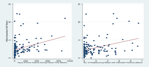
Figure 1 plots mean values for both instruments, i.e. the value of arms imports during peace time and the number of neighboring states with interstate violence, and military expenditures. Both instruments appear to positively correlate with military expenditures.

Figure 1. Trends in military Expenditure/GDP, value of Arms Flow During Peace Time & no. Of Neighboring States with interstate violence.

The strengths and statistical significance of these correlations can be examined using regression analysis. Table 3 presents regression results for the first stage military expenditure model (eq 1(1) $GR={\beta }_0+{\beta }_{1}ME/GD{P}_{it}+{\beta }_2{X}_{it}+{\delta }_i+{\mu }_{it}$(1) ). The estimated coefficients for both arms imports during peace time and the number of neighbouring states with interstate violence (lagged) are positive and statistically significant showing their strong correlations with military expenditure [Model 3.1]. To test the presence of reverse causality, the number of neighbouring states with interstate violence variable is added to the model at t and t + 1 and the estimated coefficients are statistically insignificant [Model 3.2 & Model 3.3]

Table 3. Results for military expenditure Model dependent variable: military expenditure/GDP.

	Model 3.1	Model 3.2	Model 3.3
Variables	Fixed Effect	Fixed Effect	Fixed Effect
Arms Flow During Peace Time	0.001*** (0.00)	0.001*** (0.00)	0.001*** (0.00)
No. of Neighboring States with Interstate Violencet-1	0.343** (0.01)	0.257** (0.08)	0.302* (0.05)
No. of Neighboring States with Interstate Violencet		0.152 (0.16)
No. of Neighboring States with Interstate Violencet+1			0.071 (0.52)
Other Controls	Yes	Yes	Yes
Country Fixed Effects	Yes	Yes	Yes
Years-Fixed Effects	Yes	Yes	Yes
Prob > F	0.00	0.00	0.00
Within R^2	0.25	0.25	0.25
Observations	3963	3959	3833

Notes: Constant included in the model. Other controls include GDP per capita growth rate, logged GDP per capita, inflation, logged population, ethnic fractionalization, life expectancy, non-military spending, trade openness, the intensity of conflict, dummies for the Iran-Iraq war (1980-88), post cold-war period, the financial crisis of 2008 and oil crisis/recession of 1974. Parentheses contain p values where ***p< 0.01, **p< 0.05 and *p<0.10. Driscoll Kraay’s standard errors are estimated in all models.

The results from non-IV fixed effect models are reported in Table 4. The coefficient for military expenditure is negative and statistically significant at 1 percent [Model 4.1]. In Model 4.2, the military expenditures variable is dropped and the direct effects of both instruments on economic growth are estimated which turn out to be statistically significant. However, once the military expenditures variable is included in Model 4.3 along with the instruments, the statistically significant effects of both instruments on economic growth disappear which lends support to the idea that both instruments affect economic growth indirectly through their effects on military expenditures.

Table 4. Results for economic growth models (non- IV/Full sample).

	Model 4.1	Model 4.2	Model 4.3
	Fixed Effect	Fixed Effect	Fixed Effect
Military Expenditure/GDP	−0.281*** (0.00) [0.070]		−0.251*** (0.00) [0.066]
No. of neighbouring states suffering interstate violencet-1		−0.608* (0.05) [0.311]	−0.501 (0.11) [0.310]
Arms flow during peace time		−0.001** (0.04) [0.0003]	−0.001 (0.13) [0.0003]
Other Control Variables	Yes	Yes	Yes
Country Fixed Effects	Yes	Yes	Yes
Time Dummies	Yes	Yes	Yes
With R^2	0.15	0.14	0.15
Prob > F	0.00	0.00	0.00
Observations	3985	3968	3968

Note: Constant included in the model. Other controls include GDP per capita growth rate, logged GDP per capita, inflation, logged population, ethnic fractionalization, life expectancy, non-military spending, trade openness, the intensity of conflict, dummies for the Iran-Iraq war (1980-88), post cold-war period, the financial crisis of 2008 and oil crisis/recession of 1974 Parentheses contain p value whereas brackets contain Driscoll Kraay standard errors. *** p< 0.01, ** p< 0.05 and * p<0.10.

The results from second-stage model (eq2) are reported in Table 5. As stated above, for robust inference, models are estimated using 2SLS, LIML and GMM estimators. The size of the coefficient for the military expenditures variable in Model 5.1 increases substantially in size to −1.10, which is approximately 4 times larger in magnitude than the coefficient in the fixed effect model (−1.10/-0.281 = 3.91) The statistical significance also improves as the coefficient in Model 5.1 has a p-value of less than 1 percent. Model 5.2 is estimated using the LIML estimator. There is a negligible change in size of the coefficient which remains statistically significant at 1 percent. Model 5.3 is estimated using GMM estimator. The size of the coefficient is −1.11 and it is statistically significant at 1 percent. The size of standard errors in the three models vary by a very small magnitude.

Table 5. Results for economic growth models (Iv/full sample).

	Model 5.1	Model 5.2	Model 5.3
	2SLS	LIML	GMM
Military Expenditure/GDP	−1.10*** (0.00) [0.413]	−1.11*** (0.00) [0.416]	−1.11*** (0.00) [0.412]
Other Control Variables	Yes	Yes	Yes
Country Fixed Effects	Yes	Yes	Yes
Time Dummies	Yes	Yes	Yes
Prob > F	0.00	0.00	0.00
Observations	3966	3966	3966

Note: Constant included in the model. Other controls include GDP per capita growth rate, logged GDP per capita, inflation, logged population, ethnic fractionalization, life expectancy, non-military spending, trade openness, the intensity of conflict, dummies for the Iran-Iraq war (1980-88), post cold-war period, the financial crisis of 2008 and oil crisis/recession of 1974. Parentheses contain p value whereas brackets contain Driscoll Kraay standard errors. ***p< 0.01, **p< 0.05 and *p<0.10

Diagnostic Tests

Several diagnostic tests are employed to determine the validity and strength of the instruments (Table 6). The result from the endogeneity test¹¹ supports modeling the military expenditures variable as an endogenous variable. The null hypothesis that military expenditure can be treated as an exogenous variable is rejected with a p-value of 0.03.

The result for under-identification¹² i.e. whether the excluded instruments are relevant and correlate with endogenous variable military expenditure, shows that the null hypothesis that the model is under-identified is rejected with a p value of less than 1 percent. The estimated F Statistic for the joint significance of excluded instruments is 18.16. The rule of thumb is that relatively strong instruments should have an F statistic greater than 10 (Staiger and Stock 1997). To further test the strength of the instruments, Montiel Olea and Pflueger (2013) weak instrument test is employed which is robust to both heteroscedasticity and autocorrelation. The ‘effective F statistic’ of Montiel Olea and Pflueger (2013) tests the null hypothesis that whether the asymptotic bias of an IV estimator exceeds a fraction τ of worst-case bias which will arise if the instruments are completely irrelevant. The null hypothesis that the bias from 2SLS exceeds 5 percent of worst-case bias is rejected at a 1 percent level of significance. In other words, the likelihood that the estimates are affected by a small fraction of 5 percent of worst case bias is very low. The null hypothesis of Hansen J overidentification restrictions test that instruments are uncorrelated with the errors is accepted with a p value of 0.62. Finally, in the instrument redundancy test the null hypotheses that the instruments are redundant is rejected all cases.

Controlling Heterogeneity in the Sample

Several studies have observed that the impact of military expenditure on growth can vary with respect to the political and economic conditions of countries (d’Agostino, Dunne, and Pieroni 2019; Dunne and Tian 2013). To account for such heterogeneity, the full sample is further divided into 1) developing countries¹³ 2) conflict-affected countries and 3) below-average human rights performers sub-samples.

Table 7 reports results from the developing countries’ sample. The size of the coefficient for military expenditure is −1.14 and has a p value of less than 1 percent. There is no change in the size of the coefficient in Models 7.2-7.3 which are estimated using LIML and GMM estimators. It shows that if military expenditure as a percentage of GDP in developing countries goes up by a magnitude equivalent to 1 standard deviation (3.86 percentage points), the economic growth reduces by 4.40 percentage points. In all these models, the results from the diagnostics tests suggest that instruments are valid, strong and fulfill overidentification restrictions. There are no significant differences in the size of coefficients as compared with the coefficients drawn from the full sample which suggests that the negative impact of military expenditure on economic growth is mainly driven by the developing countries sample.¹⁴

Table 6. Diagnostic Tests.

Endogeneity Test- p value Ho: ME/GDP is exogenous	0.03
Under-identification test (Kleibergen-Paap rk LM statistic) H0: Equation is under-identified	0.00
F Stat of Excluded Instrument Prob> F	18.16 (0.00)
Weak Instruments Test Montiel Pflueger Effective F Statistic H0: Bias in the estimator exceeds percentage τ of worst case bias	22.79
5% of worst case bias	α=0.01 2SLS 13.04
Hansen J Statistic- p value Ho: Instruments are valid	0.62
Instrument Redundancy Test p value
Ho: Arms transfer is redundant	0.01
Ho: Number of neighboring states with interstate violence	0.02

Table 7. Results for economic growth models (developing countries).

	Model 7.1	Model 7.2	Model 7.3
	2SLS	LIML	GMM
Military Expenditure/GDP	−1.14*** (0.00) [0.393]	−1.14*** (0.00) [0.393]	−1.14*** (0.00) [0.385]
Other Control Variables	Yes	Yes	Yes
Country Fixed Effects	Yes	Yes	Yes
Time Dummies	Yes	Yes	Yes
Prob > F	0.00	0.00	0.00
Under-identification test (Kleibergen-Paap rk LM statistic) H0: Equation is under-identified	0.01
F Stat of Excluded Instrument Prob> F	17.04 (0.00)
Weak Instruments Test Montiel Pflueger Effective F Statistic H0: Bias in the estimator exceeds percentage τ of worst case bias 5% of worst case bias	23.43 α=0.01 2SLS 12.27
Hansen J Statistic Ho: Instruments are valid	0.98
Endogeneity Test- p value Ho: ME/GDP is exogenous	0.02
Instrument Redundancy Test p value Ho: Arms transfer is redundant Ho: Number of neighboring states with interstate violence	0.001 0.0001
Observations	2881	2881	2881

Note: Constant included in the model. Other controls include GDP per capita growth rate, logged GDP per capita, inflation, logged population, ethnic factionalization, life expectancy, non-military spending, trade openness, the intensity of conflict, dummies for the Iran-Iraq war (1980-88), post cold-war period, the financial crisis of 2008 and oil crisis/recession of 1974. Parentheses contain p value whereas brackets contain Driscoll Kraay standard errors. ***p< 0.01, **p< 0.05 and *p<0.10.

Next, the sample is restricted to countries that experienced conflict episodes (more than 25 battle related deaths) for at least 1 year. The size and statistical significance of the coefficients in Models 8.1-8.3 suggest that the negative impact of military expenditures on economic growth is consistent in conflict-affected countries (Table 8).

Finally, the models are estimated for a sample of countries with below than average human rights performance. The human rights score is measured on an interval that represents the deviation from the global average set at 0. The lower the number the worse the human rights situation (Fariss 2019). The sample consists of countries that have human rights scores of less than 0 i.e. below average score. The strongest impact is observed in this sample of countries (Table 9). In Model 9.1, the size of the coefficient is −1.34. If military expenditure/GDP goes up by a magnitude equivalent to 1 standard deviation in this sample, i.e. 3.83 percentage points, then economic growth reduces by 5.12 percentage points.

Further Sensitivity Check

Additional sensitivity checks are undertaken to test the stability of the results. The trends in Figure 1 show the presence of statistical outliers. For instance, countries such as Israel, Kuwait, Oman, Saudi Arabia and Syria have very high military spending and arms imports and they may be driving the results. The model is estimated excluding these outliers (Table 10- Model 10.1) and the estimate of −1.13 is very close to the estimate of −1.14 [Model 7.1] drawn from the full developing countries sample. Finally, the temporal dimension of the sample is restricted to the 1986-2012 period. The cold-war started to wind down during the mid-1980s which was followed by large worldwide reductions in military spending (Dunne and Tian 2013).¹⁵ The results from the 1986-2012 sample continue to show a statistically significant negative effect of military spending on economic growth although the size of the coefficient slightly drops to −0.965 [Model 10.2].

Table 8. Results for economic growth models (Conflict-Affected Countries).

	Model 8.1	Model 8.2	Model 8.3
	2SLS	LIML	GMM
Military Expenditure/GDP	−0.998*** (0.00) [0.360]	−0.998*** (0.00) [0.360]	−0.976*** (0.00) [0.333]
Other Control Variables	Yes	Yes	Yes
Country Fixed Effects	Yes	Yes	Yes
Time Dummies	Yes	Yes	Yes
Prob > F	0.00	0.00	0.00
Under-identification test (Kleibergen-Paap rk LM statistic) H0: Equation is under-identified	0.01
F Stat of Excluded Instrument Prob> F	15.64 (0.00)
Weak Instruments Test Montiel Pflueger Effective F Statistic H0: Bias in the estimator exceeds percentage τ of worst case bias 5% of worst case bias	18.94 α=0.01 2SLS 12.96
Hansen J Statistic Ho: Instruments are valid	0.87
Endogeneity Test- p value Ho: ME/GDP is exogenous	0.03
Instrument Redundancy Test p value Ho: Arms transfer is redundant Ho: Number of neighboring states with interstate violence	0.01 0.02
Observations	2620	2620	2620

Note: Constant included in the model. Other controls include GDP per capita growth rate, logged GDP per capita, inflation, logged population, ethnic factionalization, life expectancy, non-military spending, trade openness, the intensity of conflict, dummies for the Iran-Iraq war (1980-88), post cold-war period, the financial crisis of 2008 and oil crisis/recession of 1974. Parentheses contain p value whereas brackets contain Driscoll Kraay standard errors. ***p< 0.01, **p< 0.05 and *p<0.10.

Table 9. Results for economic growth models (below average human rights Performers).

	Model 9.1	Model 9.2	Model 9.3
	2SLS	LIML	GMM
Military Expenditure/GDP	−1.34*** (0.00) [0.350]	−1.34*** (0.00) [0.352]	−1.33*** (0.00) [0.349]
Other Control Variables	Yes	Yes	Yes
Country Fixed Effects	Yes	Yes	Yes
Time Dummies	Yes	Yes	Yes
Prob > F	0.00	0.00	0.00
Under-identification test (Kleibergen-Paap rk LM statistic) H0: Equation is under-identified	0.004
F Stat of Excluded Instrument Prob> F	26.21 (0.00)
Weak Instruments Test Montiel Pflueger Effective F Statistic H0: Bias in the estimator exceeds percentage τ of worst case bias 5% of worst case bias	19.35 α=0.01 2SLS 11.50
Hansen J Statistic Ho: Instruments are valid	0.67
Endogeneity Test- p value Ho: ME/GDP is exogenous	0.01
Instrument Redundancy Test p value Ho: Arms transfer is redundant Ho: Number of neighboring states with interstate violence	0.02 0.005
Observations	2077	2077	2077

Note: Constant included in the model. Other controls include GDP per capita growth rate, logged GDP per capita, inflation, logged population, ethnic factionalization, life expectancy, non-military spending, trade openness, the intensity of conflict, dummies for the Iran-Iraq war (1980-88), post cold-war period, the financial crisis of 2008 and oil crisis/recession of 1974. Parentheses contain p value whereas brackets contain Driscoll Kraay standard errors. ***p< 0.01, **p< 0.05 and *p<0.10.

Table 10. Further sensitivity checks.

	Model 10.1	Model 10.2
	Excluding Outliers	1986-2012 sample
Military Expenditure/GDP	−1.13* (0.06) [0.607]	−.965*(.09)[.587] (0.09) [0.587]
Other Control Variables	Yes	Yes
Country Fixed Effects	Yes	Yes
Time Dummies	Yes	Yes
Prob > F	0.00	0.00
Weak Instruments Test Montiel Pflueger Effective F Statistic H0: Bias in the estimator exceeds percentage τ of worst case bias 5% of worst case bias	54.72 α=0.01 2SLS 4.60	53.05α=0.012SLS4.60 α=0.01 2SLS 4.60
Hansen J Statistic Ho: Instruments are valid	0.18	0.19
Observations	3802	2815

Discussion and Conclusion

Despite that there is a substantial amount of literature that examines the impact of military expenditures on economic growth, there is no empirical consensus on whether the causal impact is positive or detrimental. While heterogeneity in the findings has been attributed to variations in samples and empirical methodologies, another key issue is that of the endogeneity of military expenditures in the growth model. In a recent study d’Agostino, Dunne, and Pieroni (2019) used a dummy that captures the transition from unrest to turmoil in a country as an instrument for military expenditures and isolated a larger negative impact of military expenditure on economic growth than the one shown by the estimate obtained using OLS. However, overidentification restrictions could not be tested as the model in d’Agostino, Dunne, and Pieroni (2019) is just identified.

This study employs the value of arms imports during peace time and the number of neighboring states with interstate violence as instruments for military expenditures in the growth model. The results from IV regressions suggest that in developing countries, an annual 1 percentage point increase in military expenditure/GDP decreases economic growth by approximately 1.10 percentage points. This appears to be a strong impact if examined in terms of deviations. For instance, in a full sample, if military/expenditure goes up by 1 standard deviation (3.43 percentage points)- roughly equivalent to the yearly average military burden of Myanmar, Morocco and Armenia- then economic growth reduces by 3.77 percentage points. The findings from the models seem to support the perspective that the military burden can only be sustained at a significant cost to the economy.

Two potential extensions of this study are suggested. The current analysis is restricted to the time period 1960-2012 because the data for one of the instruments- the number of neighboring states suffering interstate violence- ends in 2012. The use of new instruments that cover the period beyond 2012 will enable examining whether the negative causal impact of military spending on growth is consistent beyond the period 2012. The size of the effects seems to vary with respect to the political conditions, for instance, the strongest negative impact of military spending on growth is observed in the sample of countries with high human rights violations. A follow up study could investigate the causes of these variations, for instance, by developing econometrics models that account for the linkages between military spending, domestic security and political environment and economic growth.

Acknowledgments

The useful comments and constructive suggestions by two anonymous referees are gratefully acknowledged. The author would also like to thank Professor Ron Smith (Birkbeck, University of London) for his feedback. The usual disclaimer applies.

Disclosure statement

No potential conflict of interest was reported by the author.

Correction Statement

This article has been republished with minor changes. These changes do not impact the academic content of the article.

Notes

1. Any violent incident is classified as organized violence where armed force was used by an organized actor against the government of an independent state resulting in at least one direct death at a specific location and a specific date

2. d’Agostino, Dunne, and Pieroni (2019) provide mathematical illustration of reverse causal impact of economic growth on military expenditure.

3. This information is taken from Arms Flow Trade Registers database of Stockholm International Peace Research Institute (SIPRI) (Stockholm International Peace Research Institute 2021). Web link- https://sipri.org/databases/armstransfers

4. In a linear regression of arms flow during the period of no active conflict, the estimated coefficient for GDP per capita growth rate is statistically insignificant.

5. See detailed trade registers of SIPRI’s arms transfer database Stockholm International Peace Research Institute (2021). The information on whether military aid financed the procurement of weapons can be found in the comment section of the trade registers.

6. The only exception is for average military expenditure/GDP which corresponds to 4 neighboring states with interstate violence. This estimate is unreliable because the number of observations for military expenditure/GDP which corresponds to 4 neighboring states with interstate violence is only 1.

7. However, they do observe a negative effect of civil wars in countries within 800 km distance on economic growth.

8. For instance, during the 1990-2002 period, civil conflicts were responsible for 90 percent of deaths in violent conflicts (Lacina 2006). Research reported on Stanford University’s website also shows that during the 1945-2002 period 16.5 million people died in civil wars as compared with 3.3 million in interstate wars. For more see https://news.stanford.edu/pr/02/civilwar925.html

9. Complete list of neighboring states for each state is provided in the annex. 2 of Major Episodes of Political Violence codebook at http://www.systemicpeace.org/inscr/MEPVcodebook2018.pdf.

10. This variable can assume negative value because the World Development Indicators (WDI) database of the World Bank calculates it by using the value of additions to the fixed assets net of inventories.

11. This test is implemented in Stata using the XTIVREG2 command. It is based on a difference of Sargan-Hansen statistics for the equation in which the suspected covariate is treated as endogenous and controls include a smaller set of instruments and for the equation in which the suspected covariate is treated as exogenous and larger set of instruments are included.

12. The statistic for this test is produced by the Stata command XTIVREG2. This is a test for the rank of a coefficients’ matrix where rejection of the null hypothesis indicates that the matrix is full column rank.

13. Countries’ classification is based on the United Nations criteria. See the annexure to World Economic Situations and Prospects (WESP) (2014) prepared by the Development Policy and Analysis Division (DPAD) of the Department of Economic and Social Affairs of the United Nations Secretariat (UN/DESA). https://www.un.org/en/development/desa/policy/wesp/wesp_current/2014wesp_country_classification.pdf

14. In the developed country sample, the estimated coefficient for military expenditure/GDP in the fixed effect model is −0.122 model and has a p value of 0.44.

15. The average global military spending/GDP was 3.51 during 1960-85 period which fell to 2.59 during 1986-2012 period.

Appendix 1

Table A1. Brief summary of literature.

Study	Coverage	Result
Selected Case Studies
Chan (1988)	Taiwan 1961-1985	Military expenditure reduces savings, investment and infrastructural development
Antonakis (1997)	Greece − 1960-1990	Negative
DeRouen (2000)	Israel 1953-1992	Negative (Short term)
Phiri	South Africa 1988-2015	Inverted U shaped relationship
Ahmed, Khorshed, Rashid, and Gow (2020)	Myanmar 1975-2014	Negative − 1 percent increase in military spending leads to 0.63 percent reduction in GDP
Selected N Sample Studies
Cappelen and Bjerkholt (1984)	17 OECD countries 1960-1980	Negative effect
Dunne and Mohammad (1995)	13 Sub-Saharan African countries 1967-1985	Negative effect (Time-Series Data), No affect (Pooled Data)
Landau (1996)	17 OECD countries, 1950-1990	Inverted U shaped relationship
Blomberg (1996)	70 countries, 1967-1982	Negative but weak effect
Stroup and Heckelman (2001)	44 African and Latin American countries, 1975-1989	Inverted U shaped relationship
Aizenman and Glick (2006)	81/83 countries, 1989-98	Positive impact in presence of security threats
Kollias et al. (2007)	15 European Countries- 1961-2000	Positive short run impact
Yakovlev (2007)	28 Countries- 1965-2000	Negative impact. Less deterimental affect when a country is net exporter of arms
Karadam et al. (2016)	Middle Eastern Countries and Turkey- 1988-2012	Inverted U shaped
Aziz and Asadullah (2017)	70 Developing Countries – 1990-2013	Negative effect- Positive effect conditional upon internal threats
d’Agostino, Dunne, and Pieroni (2019)	109 non- high income countries- 1988-2012	Negative affect

References

- Ahmed, S., A. Khorshed, A. Rashid, and J. Gow. 2020. “Militarisation, Energy Consumption, CO2 Emissions and Economic Growth in Myanmar.” Defence and Peace Economics 31 (6): 615–641.
- Aizenman, J., and R. Glick. 2006. “Military Expenditure, Threats and Growth.” The Journal of International Trade & Economic Development 15 (2): 129–155.
- Antonakis, N. 1997. “Military Expenditure and Economic Growth in Greece, 1960-1990.” Journal of Peace Research 34 (1): 89–100.
- Arellano, M., and S. Bond. 1991. “Some Tests of Specification for Panel Data: Monte Carlo Evidence and an Application to Employment Equation.” The Review of Economic Studies 58 (2): 277–297.
- Aziz, N., and M. N. Asadullah. 2017. “Military Spending, Armed Conflict and Economic Growth in Developing Countries in the Post-Cold War Era.” Journal of Economic Studies 44 (1): 47–68.
- Benoit, E. 1973. Defence and Economic Growth in Developing Countries. Boston: Lexington Books.
- Benoit, E. 1978. “Growth and Defence in LDCs.” Economic Development & Cultural Change 26 (2): 271–280.
- Blomberg, S. B. 1996. “Growth, Political Instability and the Defence Burden.” Economica 63 (252): 649–672.
- Cameron, A. C., and P. K. Trivedi. 2009. Microeconometrics Using Stata. Texas: A Stata Press Publication.
- Cappelen, A. G., and O. Bjerkholt. 1984. “Military Spending and Economic Growth in OECD Countries.” Journal of Peace Research 21 (4): 361–373.
- Center for Systemic Peace. 2019. Major Episodes of Political Violence, 1946-2018. Vienna (USA): Center for Systemic Peace. https://www.systemicpeace.org/inscrdata.html.
- Chan, S. 1988. “Defense Burden and Economic Growth: Unraveling the Taiwanese Enigma.” The American Political Science Review 82 (3): 913–920.
- Chang, H.-C., B.-N. Huang, and C. W. Yang. 2011. “Military Expenditure and Economic Growth Across Different Groups: A Dynamic Granger-Causality Approach.” Economic Modelling 28 (6): 2416–2423.
- Conte, A., and S. Migali. 2019. “The Role of Conflict and Organized Violence in International Forced Migration.” Demographic Research 41: 393–424.
- d’Agostino, G., J. P. Dunne, and L. Pieroni. 2019. “Military Expenditure, Endogeneity and Economic Growth.” Defence and Peace Economics 30 (5): 509–524. https://doi.org/10.1080/10242694.2017.1422314.
- DeRouen, K. J. 2000. “The Guns-Growth Relationship in Israel.” Journal of Peace Research 37 (1): 69–83.
- Drazanova, L. 2019. “Historical Index of Ethnic Fractionalization Dataset (HIEF.” Harvard Dataverse. https://doi.org/10.7910/DVN/4JQRCL.
- Driscoll, J., and A. C. Kraay. 1998. “Consistent Covariance Matrix Estimation with Spatially Dependent Data.” The Review of Economics and Statistics 80 (4): 549–560.
- Dunne, P., and N. Mohammad. 1995. “Military Expenditure in Sub-Saharan Africa: Some Evidence for 1967-1985.” Journal of Peace Research 32 (3): 331–343.
- Dunne, P., R. Smith, and D. Willenbockel. 2005. “Models of Military Expenditure and Growth: A Critical Review.” Defense and Peace Economics 16 (6): 449–462.
- Dunne, J., and N. Tian. 2013. “Military Spending and Economic Growth: A Survey.” The Economics of Peace & Security Journal 8 (1): 5–11.
- Dunne, P. J., and N. Tian. 2013. “Military Expenditure and Economic Growth: A Survey.” The Economics of Peace & Security Journal 8 (1). https://doi.org/10.15355/epsj.8.1.5.
- Dunne, J., and M. Uye. 2009. “Defence Spending and Development.” In The Global Arms Trade, edited by T. Andrew, 293–305. Abindon: Routledge. https://doi.org/10.4324/9780203851456-25.
- Fariss, C. J. 2019. “Yes, Human Rights Practices are Improving Over Time.” The American Political Science Review 113 (3): 868–881.
- Karadam, D. Y., J. Yildirim, and N. Ocal. 2016. “Military Expenditure and Economic Growth in Middle Eastern Countries and Turkey: A Non-Linear Panel Data Approach.” Defence and Peace Economics 28 (6): 719–730.
- Kollias, C., N. Mylonidis, and S.-M. Paleologou. 2007. “A Panel Data Analysis of the Nexus Between Defence Spending and Growth in the European Union.” Defence and Peace Economics 18 (1): 75–85.
- Kreutz, J. 2010. “How and When Armed Conflicts End: Introducing the UCDP Conflict Termination Dataset.” Journal of Peace Research 47 (2): 243–250.
- Lacina, B. 2006. “Explaining the Severity of Civil Wars.” The Journal of Conflict Resolution 50 (2): 276–289.
- Landau, D. 1996. “Is One of the Peace Dividends Negative? Military Expenditure and Economic Growth in the Wealthy OECD Countries.” The Quarterly Review of Economics & Finance 36 (2): 183–195.
- Mani, K. 2007. “Militaries in Business: State-Making and Entrepreneurship in the Developing World.” Armed Forces & Society 33 (4): 591–611.
- Montiel Olea, J. L., and C. E. Pflueger. 2013. “A Robust Test for Weak Instruments.” Journal of Business & Economic Statistics 31 (3): 358–369.
- Moon, C.-I., and S. Lee. 2009. “Military Spending and the Arms Race in Korean Peninsula.” Asian Perspectives 33 (4): 69–99.
- Murdoch, J. C., and T. Sandler. 2004. “Civil Wars and Economic Growth: Spatial Dispersion.” American Journal of Political Science 48 (1): 138–151.
- Phillips, B. J. 2015. “Civil War, Spillover and Neighbors’ Military Spending.” Conflict Management and Peace Science 32 (4): 425–442.
- Phiri, A. 2019. “Does Military Spending Nonlinearly Affect Economic Growth in South Africa?” Defence and Peace Economics 30 (4): 474–487.
- Ram, R. 1995. “Defense Expenditure and Economic Growth.” In Handbook of Defense Economics, edited by R. Ram, 251–273. Amsterdam: Elsevier.
- Smaldone, J. P. 2006. “African Military Spending: Defence versus Development.” African Security Review 15 (4): 18–32.
- Smith, R. P. 2017. “Military Expenditure Data: Theoretical and Empirical Considerations.” Defence and Peace Economics 28 (4): 422–428.
- Staiger, D., and J. H. Stock. 1997. “IV Regressions with Weak Instruments.” Econometrica 65 (3): 557–586.
- Stockholm International Peace Research Institute. 2021. SIPRI Arms Transfer Database. Stockholm: Stockholm International Peace Research Institute.
- Stroup, M. D., and J. C. Heckelman. 2001. “Size of the Military Sector and Economic Growth: A Panel Data Analysis of Africa and Latin America.” Journal of Applied Economics 4 (2): 329–360.
- Trebilcock, C. 1969. “Spin-Off in British Economic History: Armaments and Industry, 1760-1914.” The Economic History Review 22 (3): 474–490.
- Trebilcock, C. 1973. ““British Armaments and European Industrialization.” Economic History Review 26 (2): 254–272.
- The United Nations. 2014. World Economic Situation and Prospects. New York: The United Nations.
- The World Bank. 2021. World Development Indicators Database. Washington, DC: The World Bank. https://databank.worldbank.org/reports.aspx?source=world-development-indicators.
- Yakovlev, P. 2007. “Arms Trade, Military Spending and Economic Growth.” Defence and Peace Economics 18 (4): 317–338.