
 ?Mathematical formulae have been encoded as MathML and are displayed in this HTML version using MathJax in order to improve their display. Uncheck the box to turn MathJax off. This feature requires Javascript. Click on a formula to zoom.
Abstract
A highly accurate human hand kinematics model and identification are proposed. The model includes the five digits and the palm arc based on mapping function between surface landmarks and estimated joint centres of rotation. Model identification was experimentally performed using a motion tracking system. The evaluation of the marker position estimation error, which is on sub-millimetre level across all digits, underlines model quality and accuracy. Noticeably, with the development of this model, we were able to improve various modelling assumptions from literature and found a basic linear relationship between surface and skeleton rotational angles.
1. Introduction
The analysis and evaluation of human hand kinematics is essential for developing human-like smart prostheses and articulated robotic hands. The kinematic complexity of the human hand makes accurate modelling a challenging task. Despite that tremendous progress has been made, a complete and accurate kinematics model with its corresponding identification procedure is still lacking. In fact, limitations are still present in the state of the art as follows.
| (1) | Specific types of isolated joints such as metacarpophalangeal (MCP) (Speirs et al. Citation2001) or 2nd–5th digits (Braido and Zhang Citation2004) or specific digits (Parasuraman and Zhen Citation2009; Nataraj and Li Citation2013, Citation2015) were considered. More extended models with varying modelling assumptions and accuracy were also developed, see Table . | ||||
| (2) | The thumb has been modelled with different assumptions regarding its number of degrees of freedom (DoFs). The state-of-the-art thumb models include 4 DoFs (Cerveri et al. Citation2007; Metcalf et al. Citation2008; Cobos et al. Citation2010) and 5 DoFs (Miyata et al. Citation2004; Veber and Bajd Citation2006; Parasuraman and Zhen Citation2009; Cordella et al. Citation2014; Peña Pitarch et al. Citation2014), see Table . Yet, a highly accurate thumb model is still lacking. Moreover, some thumb models did not relate it to its own reference system (Carpinella et al. Citation2006; Veber and Bajd Citation2006; Cordella et al. Citation2014). In fact, thumb movements in the plane of the hand may occur as a result of combined joint movements (Kuczynski Citation1974). Thus, a separate coordinate system is required to describe motions at the trapeziometacarpal (TM) joint (Cooney et al. Citation1981). | ||||
| (3) | Finger joint centres of rotation (CoRs) cannot be simply substituted by surface landmark positions (Supuk et al. Citation2004) and estimation of CoRs is important in describing the skeletal kinematics (Zhang et al. Citation2003). Available CoR estimation includes simple translation (Cerveri et al. Citation2007), optimisation routines (Zhang et al. Citation2003; Supuk et al. Citation2004), and optimisation with circle intersection (Miyata et al. Citation2004; Veber and Bajd Citation2006). However, no forward and inverse functions between surface landmarks and CoRs were proposed in the aforementioned works. Furthermore, thumb joint CoRs have not been identified yet. | ||||
| (4) | The need for specially designed experimental set-ups (Degeorges et al. Citation2005; Shen et al. Citation2012; Nataraj and Li Citation2013). | ||||
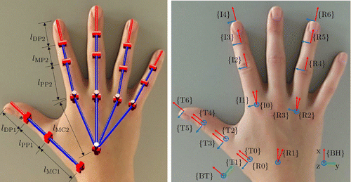
Figure 1. The proposed human hand kinematics model with 26 DoFs. Left: representation of the serial linkages for each digit, which is assumed to be a rigid body segment. The 2nd–5th digits have 4 DoFs (2 DoFs for MCP joint F/E and Ab/Ad and 2 DoFs for PIP and DIP joints F/E), while the 1st digit has 6 DoFs (2 DoFs for F/E and Ab/Ad for each joint). In the thumb model, the Ab/Ad of the IP joint is considered passive (indicated by ‘’) while the other 5 DoFs are actuated. The palm arc is modelled as Ab/Ad and F/E of the two palm joints. Right: coordinate systems for each digit and the hand base. The alphabet in the CS naming indicates the digit initial.
Contribution. This paper aims to provide and validate a highly accurate human hand kinematics model. Specifically, our contributions are as follows.
| (1) | Developing a complete accurate hand model, including the four fingers (4 DoFs each ), the thumb (6 DoFs) and the palm arc (4 DoFs), see Table . | ||||
| (2) | Designing a highly accurate thumb kinematics model associated to its own frame of reference, which is identified in subject-specific relationships to the hand dorsal reference frame. Based on an in-depth literature review, this is to the authors’ knowledge the first study investigating such relationships using a motion tracking technique. | ||||
| (3) | Highlighting the effect of considering passive DoF on the kinematics model accuracy, i.e. additional passive DoF in the thumb. This formalises a first hint towards joint flexibility. | ||||
| (4) | Proposing a systematic flexion/extension CoR estimation algorithm and the forward and inverse kinematics mapping between surface and skeleton kinematics. | ||||
| (5) | Proposing a practical identification procedure for standard motion tracking techniques. | ||||
Table 1. State-of-the-art hand kinematics models.
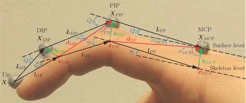
Figure 2. Two-dimensional finger schematic diagram.
2. Methods
2.1. Hand biomechanics and modelling assumptions
A human hand is composed of five digits and the palm. The 2nd–5th digits have three joints with 4 DoFs of MCP flexion/extension (F/E) and abduction/adduction (Ab/Ad), proximal interphalangeal (PIP) F/E, and distal interphalangeal (DIP) F/E (Lippert Citation2011). Thumb and palm arc biomechanics and modelling assumptions are discussed as in the following.
Thumb. The thumb has three joints with more complex DoFs. The carpometacarpal (CMC) (or TM joint) has 2 DoFs (F/E and Ab/Ad) and permits some axial rotation (Lippert Citation2011). The MCP joint has 2 DoFs (Kapandji Citation2007) and might be modelled as 1 DoF (Cobos et al. Citation2010). In our pilot experiments, we found that the thumb has significant passive DoF (elastic behaviour which might originate from joint capsule elasticity) which occur in interphalangeal (IP) joint during physical interactions between objects and thumb. Such interactions result in thumb distal phalange pronation, which is modelled by 1 passive DoF (Ab/Ad) in the IP joint. Thus, the proposed thumb model has 6 DoFs (1 passiveFootnote1 and 5 actuatedFootnote2 DoFs). To show the importance of the additional 1 passive DoF and the accuracy of the proposed 6 DoFs thumb model in comparison with the state-of-the-art thumb models, the following three models are compared and discussed (Section 3.2):
4 DoF thumb model (4 actuated DoFs, without passive DoFs),
5 DoF thumb model (5 actuated DoFs, without passive DoFs),
6 DoF thumb model (5 actuated DoFs, with 1 passive DoF).
Two DoFs where the palm arc is modelled,
A static joint where the palm arc is not modelled.
2.2. Surface and skeletal kinematics model
The proposed model connects two representation levels, namely the skeletal level and the surface level, see Figure . These correspond to centres of rotation and skin landmarks, respectively. For obvious reasons, it is chosen to be the skeletal joint position vector and the set of surface Cartesian positions
. Furthermore, the two auxiliary coordinates surface joint configuration
and the set of joint CoR positions
are introduced. The desired mapping
is divided into composable sub-mappings. Overall two different types of mappings are categorised as follows.
| (1) | Intra-level mappings:
| ||||||||||||||||
| (2) | Inter-level mapping: denoting the transition between surface level and skeletal level representations | ||||||||||||||||
Figure 3. Block diagram of model identification and validation.
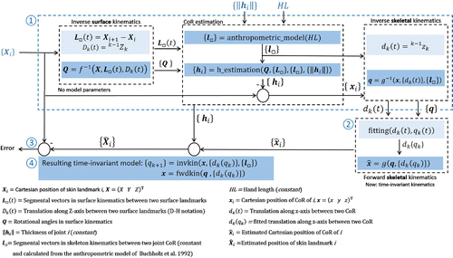
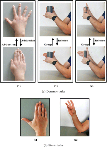
Figure 4. Maker placement and labelling.
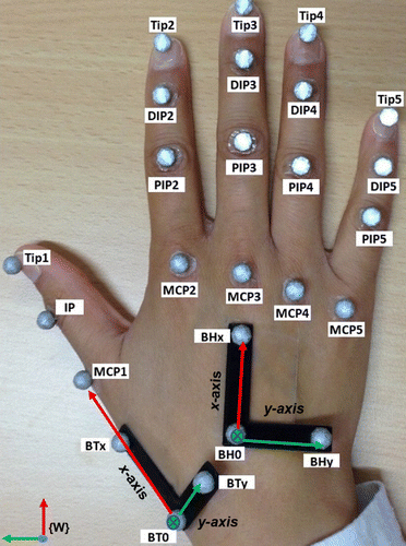
Figure 5. Experimental tasks.
2.2.1. Intra-level mapping
Surface Kinematics. Surface kinematics describe the relationship between the skin landmark Cartesian positions and the surface joint configuration
:
(1a)
(1a)
(1b)
(1b)
(1c)
(1c)
(1d)
(1d) where
and
denote the forward and inverse surface kinematics, respectively. In order to find
and
, two base frames and one frame for each joint DoF are established, see Figure . These base frames are the Hand Base frame
and the Thumb Base frame
, which are related to each other via:
(2)
(2)
where denotes the rotation matrix.
denotes the vector pointing from the origin of
to the origin of
, represented by BT0. Joint DoF frames are determined by transforming from the base frames via
(3)
(3)
together with the classical Denavit–Hartenberg (D–H) convention (Reddy Citation2014). The D–H parameters are listed in Table A1. Then, homogeneous transformation matrices can be formulated as a function of
. Equation (Equation3
(3)
(3) ) can be solved for
by using the property
, i.e. being the origin of frame k, and by assuming
to be known, see Appendix 2.
Skeletal kinematics. The skeletal kinematics connects Cartesian positions of joint CoR with the skeletal joint configuration
, i.e.
(4a)
(4a) where
and
are the skeletal forward and inverse kinematics, respectively. In order to find them, similarly to the surface kinematics, a set of reference frames isestablished; however, with a different D–H parameter set, see Table A2. Analogous to the surface kinematics, the homogeneous transformation matrix
is a function of
, and (Equation5
(5)
(5) ) can be solved for
by knowing
as the origin of frame k, and
from inter-level mapping (Section 2.2.2).
(4b)
(4b)
2.2.2. Inter-level mapping
In the previous section surface and skeletal kinematics were introduced. The mapping between these two levels is done by the inter-level mapping. Figure depicts surface and skeletal level positions, which are related to each other by the vectors as
(4c)
(4c)
The estimation of is performed in 2-D space to minimise the number of unknowns (Zhang et al. Citation2003). For the 2nd–5th digits, the best frame for 2-D projection is MCP F/E frame, defined as
, where F/E occurs and one moves with Ab/Ad motion accordingly. The thumb has Ab/Ad DoF in each joint which make the F/E motion in different planes. Thus, the CoR of CMC is calculated in frame
, while the CoR of MCP and IP joints are obtained in frames
and
, respectively, see Figure . In the 2-D spaces (Figure ), the Law of Cosines and dot product are used to estimate
as explained in Appendix 3.
Figure 6. Comparison between measured and estimated in two models of the 2nd palm joint. Top: static joint model (without considering palm arc). Bottom: 2 DoF joint model (with considering palm arc). The figure shows the pinky finger of an exemplar subject expressed in
.
2.3. Model identification and validation
Obviously, the simultaneous measurement of motion capture data with online high frequency imaging for model validation would be ideal for validation. However, since this is technically not feasible, especially for high-frequency motions, our algorithm is evaluated according to the consistency scheme shown in Figure . The model self-consistency and accuracy are evaluated as follows: in the inverse calculation path, only measurements ,
, and HL serve as the input to estimate the skeletal joint position
, whereas in the forward calculation path,
and the calibrated kinematics model with fitted model relation
are required to estimate
. The difference between
and
quantifies model consistency and accuracy. The practical identification procedure was performed as follows.
2.3.1. Algorithmic identification procedure
In the proposed model, two floating base coordinate systems are used: and
, see Figure . The identification of
is performed at every time step, while
is established by defining a rotation matrix between
and
in the reference posture as explained in Appendix 4. Thereafter, the overall identification procedure that estimates the joint angles
from measured marker positions
is performed, see Appendix 4.
2.3.2. Experimental setup
Nine healthy subjects (7 males and 2 females, age years with hand length (
mm) volunteered for this study. All participants provided written consent prior to their participation. The test procedures were conducted according to the guidelines of the Declaration of Helsinki and approved by the ethics committee of Leibniz Universität Hannover, Germany.
Twenty-five reflective spherical markers were attached on specific bony landmarks, see Figure . In the five digits, markers were attached to the heads of metacarpals and of phalanges as suggested by Metcalf et al. (Citation2008). In each trial, marker coordinates were acquired during two static and three dynamic tasks using an optoelectronic motion capture system (©Vicon Motion Systems Ltd., UK with its associated software Nexus 2.0), see Figure .
3. Results and discussions
The block diagram of model identification and validation is shown in Figure . The sub-millimetre difference between and
indicates that the proposed model and associated identification procedure are consistent and highly accurate. This also validates the proposed CoRs estimation algorithm, which is part of the model. The detailed results and discussions of the individual assumptions follow now.
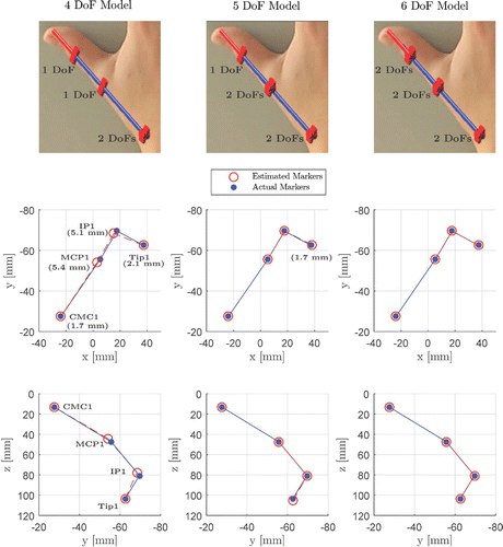
Figure 7. Comparison between measured and estimated expressed in
for 4 DoF (left), 5 DoF (middle) and 6 DoF (right) thumb models for an exemplar subject. The top row shows a representation of the serial linkage of the compared three models. The estimation error, defined as the maximal Euclidean distance between measured and estimated
, is represented by the numbers in brackets for the corresponding
.
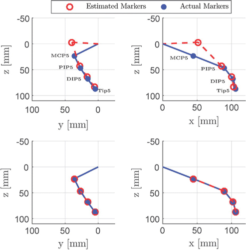
3.1. Palm arc modelling
The aim of this section is to highlight the effect that modelling the palm arc has on the pose estimation accuracy of the pinky finger. The difference between the estimated and measured during Task S2, resulted from the compared models of the 2nd palm joint, is depicted in Figure . In the static palm joint model, the error in terms of the Euclidean norm among different subjects is up to 65.0, 20.0, 10.6 and 9.3 mm for
,
,
and
, respectively. As one may notice,
exhibits the largest error, especially along the z-axis of
coordinate system, see Figure top. This phenomenon emphasises that the static joint model estimates
on the x–y plane of the
(z-component close to zero), while the true position is shifted downwards to form the palm arc. In our proposed 2 DoF model, only sub-millimetre errors could be observed between estimated and measured
, see Figure bottom.
Figure 8. Comparison between and the estimated
in Tasks D1 (left) and D2 (right). This figure shows segment lengths of an exemplar index finger. Segment lengths are compared to anthropometrically modelled segment lengths (Buchholz et al. Citation1992).
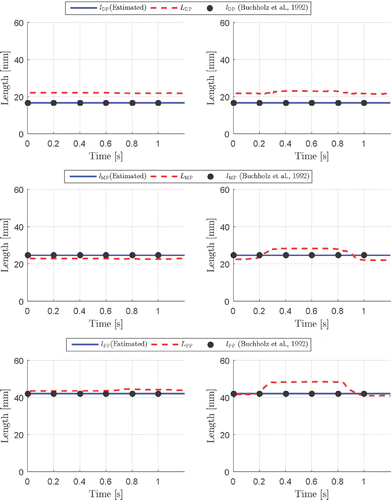
Figure 9. Skeleton rotational angles with respect to surface rotational angles
in Task D2. Columns indicate fingers (left to right): index, middle, ring and pinky. Rows indicate rotational angles (top to bottom): DIP F/E, PIP/F/E and MCP F/E. For MCP Ab/Ad, the rotational rotation angles on surface level and skeleton level are equal with
, thus they are not shown in this figure.
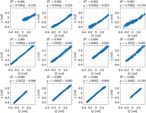
Figure 10. Skeleton rotational angles with respect to surface rotational angles
in Task D3. Columns indicate fingers (left to right): index, middle, ring and pinky. Rows indicate rotational angles (top to bottom): DIP F/E, PIP/F/E, and MCP F/E. For MCP Ab/Ad, the rotational rotation angles on surface level and skeleton level are equal with
, thus they are not shown in this figure.
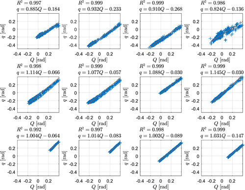
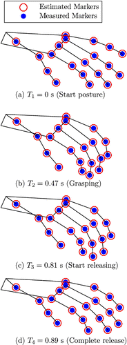
Figure 11. Comparison between measured and estimated in Task D2 for an exemplar subject at different instants (from
to
).
3.2. Thumb modelling
In this section, thumb modelling results and considerations are discussed as follows.
Rotational relationship between and
. The identification of
is shown in Algorithm 1. A difference ranging between 10.6
and 24.3
Footnote3 was noticed in
among subjects which is probably caused by the variation in population and marker placement. Conclusively, it would be more accurate to identify
for each subject rather than using fixed values. This identification results in an adaptable model which minimises the effect of individual variations.
Thumb model DoFs and accuracy. The difference between the estimated and measured in the comparedthree thumb models is shown in Figure . From there, it becomes clear that the insufficient number of DoFs affects the accuracy of the model. In the 4 DoF model an error is observed in all
due to not considering the Ab/Ad of MCP1 and IP joints. Compared to the 4 DoF model, the 5 DoF model shows improved accuracy in all
, nearly to almost negligible error except in
. This is due to the absence of IP Ab/Ad DoF. Despite that the IP joint has been modelled as single DoF in the available thumb models (Miyata et al. Citation2004; Cerveri et al. Citation2007; Metcalf et al. Citation2008; Parasuraman and Zhen Citation2009; Cobos et al. Citation2010; Cordella et al. Citation2014), considering the Ab/Ad is of vital importance to reconstruct tip positions accurately. In our pilot experiment, a combination of F/E and Ab/Ad at IP joint was observed, especiallyduring physical interactions between the thumb segments and the grasped object, where the DP of thumb rolls over the object’s surface to achieve a stable grasp. This phenomenon might be related to elastic joint capsules. Besides, there are non-constant bone segment lengths being reconstructed by 4 DoF and 5 DoF models. To tackle these issues, a 6 DoF model is proposed which includes 5 active DoFs and 1 passive DoF. The proposed thumb model has an improved accuracy in all
compared to the other two models (4 DoF and 5 DoF models), see Figure . Compared to the literature models (Table ) our proposed 6 DoF model has proved to provide significantly better accuracy with no difference was noticed between measured and estimated
.
Table 2. Comparison of accuracy among different models from literature.
3.3. Surface kinematics and skeleton kinematics
In this section, segment lengths, joint rotational angles and Cartesian errors are compared between surface and skeleton kinematics.
Segment lengths. Surface segmental length are different from
, see Figure . This difference supports our hypothesis that surface kinematics is not the same as skeletal kinematics. Surface segmental length
varies over time due to:
| (1) | skin displacement relative to skeleton, and | ||||
| (2) | rotation of markers about the DoF axes during movements. | ||||
Joint rotational angles. The relationship between and
in Tasks D2 and D3 is shown in Figures and . Experimental data revealed a highly linear relationship between F/E angles in all joints with
in most of joints. From the linear regression coefficients, the difference between
and
in terms of both slopes and intersects is clear.
Errors in Cartesian space. The Cartesian errors are calculated as the difference between marker positions () estimated by the forward kinematics model and the positions directly measured by the motion capture system, see Figure . In surface kinematics, an error increase has been noticed along the serial chain from MCP landmark to tip of 2nd–5th digits (Cerveri et al. Citation2007; Cordella et al. Citation2014). This can be explained by finger curvature (Cordella et al. Citation2014), which is equivalent to
and
in the used D–H notation (Appendix 1). To overcome this issue, in the proposed model
is calculated based on the experimental measurements from motion tracking data, while
is fitted as a function of
(in our case polynomial regression), see Figure . This improves the model accuracy to a sub-millimetre error in most cases. Only in one case, an error of nearly 2 mm was observed due to the improper
–
fitting. This, however, could be solved easily with more complex fitting algorithms. In addition, the variance of
during tasks should be further investigated with respect to joint DoFs, joint capsule elasticity and physical finger-object interaction in the future.
Compared to the available and comparable models in the literature (Table ), our proposed model has proved to be highly accurate without a noticeable difference between measured and estimated , see Figure . This sub-millimetre accuracy evidences the model self-consistency (see Figure ) and, ergo, reliable skeletal
can be obtained by using the proposed method.
4. Conclusion
An accurate human hand kinematics model, including the four fingers (4 actuated DoFs each), the thumb (5 actuated DoFs and 1 passive DoF) and the palm arc (4 actuated DoFs), has been proposed along with an identification procedure that estimates joint CoRs. These estimated CoRs are part of the mapping functions between surface and skeleton kinematics. With the identification and validation scheme, the accuracy of sub-millimetre level indicates that the proposed model and associated identification procedure are consistent and highly accurate. The proposed thumb model with the 5 actuated DoFs and the 1 passive DoF has significantly improved accuracy compared to existing thumb models. Despite the fact that we did not investigate similar passive movements in the other digits, the passive DoFs obviously exist in the other digits. Future work will address: (1) the passive DoFs and their elasticity in all hand joints and (2) the changes of during tasks with respect to joint DoFs, joint capsule elasticity and physical finger-object interactions. Besides, the identification will be more efficient, when
can be automatically estimated instead of manual measurement.
hand_kinematics.mp4
Download MP4 Video (3.7 MB)Additional information
Funding
Notes
We hereby declare that all authors of this paper have no financial or personal relationships with other people or organizations that could inappropriately influence (bias) our work.
Supplemental data for this article can be accessed at https://doi.org/10.1080/10255842.2018.1425996
1 A passive DoF is a flexible joint that is not actuated by muscles.
2 An actuated or active DoF is a joint that is actuated by muscles.
3 The angular difference is defined as , where
and
denote the quaternions of two rotation matrices, and
is the inner product.
Related Research Data
References
- Braido P, Zhang X. 2004. Quantitative analysis of finger motion coordination in hand manipulative and gestic acts. Human Mov Sci. 22:661–678.
- Buchholz B, Armstrong TJ, Goldstein SA. 1992. Anthropometric data for describing the kinematics of the human hand. Ergonomics. 35(3):261–273.
- Carpinella I, Mazzoleni P, Rabuffetti M, Thorsen R, Ferrarin M. 2006. Experimental protocol for the kinematic analysis of the hand: definition and repeatability. Gait Posture. 23:445–454.
- Cerveri P, Momi ED, Lopomo N, Baud-Bovy G, Barros RML, Ferrigno G. 2007. Finger kinematic modeling and real-time hand motion estimation. Ann Biomed Eng. 35(11):1989–2002.
- Cobos S, Ferre M, Sánchez-Urán MA, Ortego J, Aracil R. 2010. Human hand descriptions and gesture recognition for object manipulation. Comput Methods Biomech Biomed Eng. 13(3):305–317.
- Cooney WP, Lucca MJ, Chao EYS, Linscheid RL. 1981. The kinesiology of the thumb trapeziometacarpal joint. J Bone Joint Surg. 63-A(9):1371–1381.
- Cordella F, Zollo L, Salerno A, Accoto D, Guglielmelli E, Siciliano B. 2014. Human hand motion analysis and synthesis of optimal power grasps for a robotic hand. Int J Adv Robot Syst. 11(37):1–13.
- Degeorges R, Parasie J, Mitton D, Imbert N, Goubier J-N, Lavaste F. 2005. Three-dimensional rotations of human three-joint fingers: an optoelectronic measurement. preliminary results. Surg Radiol Anat. 27(1):43–50.
- Kapandji AI. 2007. The physiology of the joints: annotated diagrams of the mechanics of the human joints. 6th ed. Vol. 1. London: Churchill Livingstone.
- Kuczynski K. 1974. Carpometacarpal joint of the human thumb. J Anat. 118:119–126.
- Levangie PK, Norkin CC. 2005. Joint structure and function: a comprehensive analysis. 4th ed. Philadelphia (PA): F.A. Davis Co.
- Lippert LS. 2011. Clinical kinesiology and anatomy. 5th ed. Philadelphia (PA): F. A. Davis Co.
- Metcalf CD, Notley SV, Chappell PH, Burridge JH, Yule VT. 2008. Validation and application of a computational model for wrist and hand movements using surface markers. IEEE Trans Biomed Eng. 55(3):1199–1210.
- Miyata N, Kouchi M, Kurihara T, Mochimaru M. 2004. Modeling of human hand link structure from optical motion capture data. Proceedings of 2004 IEEE/RSJ International Conference on Intelligent Robots and Systems; Sendai, Japan. p. 2129–2135.
- Nataraj R, Li Z-M. 2013. Robust identification of three-dimensional thumb and index finger kinematics with a minimal set of markers. J Biomed Eng. 135(9):0910021–0910029.
- Nataraj R, Li Z-M. 2015. Integration of marker and force data to compute three-dimensional joint moments of the thumb and index finger jigits during pinch. Comput Methods Biomech Biomed Eng. 18(16):592–606.
- Parasuraman S, Zhen CCS. 2009. Development of robot assisted hand stroke rehabilitation system. International Conference on Computer and Automation Engineering. Bangkok. Thailand.
- Pe\~{n}a Pitarch E, FalgueraNT, Yang JJ. 2014. Virtual human hand: model and kinematics. Comput Methods Biomech Biomed Eng. 17(5):568-579.
- Pe\~{n}a Pitarch E, YangJ, Abdel-Malek K. 2005. Santos™ hand: a 25 degree-of-freedom model. Proc. of SAE Digital Human Modeling for Design and Engineering. Iowa City, USA.
- Reddy AC. 2014. Difference between Denavit--Hartenberg (D--H) classical and modified conventions for forward kinematics of robots with case study. International Conference on Advanced Materials and manufacturing Technologies (AMMT); Dec; Chandigarh, India: JNTUH College of Engineering Hyderabad.
- Shen ZL, Mondello TA, Nataraj R, Domalain MF, Li Z-M. 2012. A digit alignment device for kinematic analysis of the thumb and index finger. Gai. 36:643–645.
- Speirs AD, Small CF, Bryant JT, Pichora DR, Zee BY. 2001. Three-dimensional metacarpophalangeal joint kinematics using two markers on the phalanx. J Eng Med. 2015(4):415–419.
- Supuk TG, Harwin W, Zanchi V. 2004. Calculating positions of the finger joints centres of rotations in flexion-extension movement from reflective markers. Proceedings of The IMEKO, IEEE, SICE 2nd International Symposium on Measurement, Analysis and Modeling of Human Functions; Genova, Italy. p. 363–366.
- Veber M, Bajd T. 2006. Assessment of human hand kinematics. Proceedings of the 2006 IEEE International Conference on Robotics and Automation; May; Orlando, FL. p. 2966–2971.
- Veber M, Bajd T, Munih M. 2006. Assessment of finger joint angles and calibration of instrumental glove. Advances in Robot Kinematics; New York (NY): Springer-Verlag New York Inc. p. 185–192.
- Zhang X, Lee S-W, Braido P. 2003. Determining finger segmental centers of rotation in flexion-extension based on surface marker measurement. Journal of Biomechanics. 36:1097–1102.
Appendix 1
D–H parameters
Table A1. D–H parameters of surface kinematics.
Table A2. D–H parameters of skeletal kinematics.
Appendix 2
Solving for rotational angles
Q’s for 1st digit. The 6 DoFs of the thumb are calculated as in (EquationB1a(B1a)
(B1a) )–(EquationB1f
(B1f)
(B1f) ).
(4d)
(4d)
(5)
(5)
(6)
(6)
(B1a)
(B1a)
(B1b)
(B1b)
(B1c)
(B1c) where
: is the x-component of MCP landmark position in {0}
: is the y-component of MCP landmark position in {0}
: is the z-component of MCP landmark position in {0}
: is the x-component of IP landmark position in {2}
: is the y-component of IP landmark position in {2}
: is the z-component of IP landmark position in {2}
: is the x-component of Tip landmark position in {4}
: is the y-component of Tip landmark position in {4}
is calculated by (Equation3
(3)
(3) ) and the transformation matrix
.
is calculated by (Equation3
(3)
(3) ) and the
from the previous steps.
Q’s for 2nd–3rd digits. The 4 DoFs are calculated as in (EquationB2a(B2a)
(B2a) –EquationB2d
(B2d)
(B2d) ).
(B1d)
(B1d)
(B1e)
(B1e)
(B1f)
(B1f)
(B2a)
(B2a) where
: is the x-component of PIP landmark position in {0}
: is the y-component of PIP landmark position in {0}
: is the z-component of PIP landmark position in {0}
: is the x-component of DIP landmark position in {2}
: is the y-component of DIP landmark position in {2}
: is the x-component of Tip landmark position in {3}
: is the y-component of Tip landmark position in {3}
is calculated by (Equation3
(3)
(3) ) and the transformation matrix
.
is calculated by (Equation3
(3)
(3) ) and the
from the previous steps.
Q’s for 4th–5th digits. Equations (EquationB3a(B3a)
(B3a) )–(EquationB3f
(B3f)
(B3f) ) are used to calculate the rotational angles as follows:
(B2b)
(B2b)
(B2c)
(B2c)
(B2d)
(B2d)
(B3a)
(B3a)
(B3b)
(B3b)
(B3c)
(B3c) where
: is the x-component of MCP landmark position in {B}
: is the y-component of MCP landmark position in {B}
: is the z-component of MCP landmark position in {B}
: is the x-component of PIP landmark position in {2}
: is the y-component of PIP landmark position in {2}
: is the z-component of PIP landmark position in {2}
: is the x-component of DIP landmark position in {4}
: is the y-component of DIP landmark position in {4}
: is the x-component of Tip landmark position in {5}
: is the y-component of Tip landmark position in {5}
is calculated by (Equation3
(3)
(3) ) and the
from the previous steps.
Appendix 3
Estimation of 
The calculations of the vector are detailed in this section for different joints of the 2nd to 5th digits. Considering the difference in defining the joint F/E plane in the thumb joints, the vector
is estimated analogous to the other fingers. Figure shows the finger 2-D F/E plane and parameters definition to calculate
. the vector
for joints of 2nd–5th digits is calculated as follows.
DIP joint. The vector is defined as
(B3d)
(B3d)
The unit vector can be obtained as in Supuk et al. (Citation2004) from
(B3e)
(B3e)
(B3f)
(B3f) as
(C1)
(C1)
where is obtained from the Law of Cosines as
(C2a)
(C2a)
and from
(C2b)
(C2b) PIP joint. Analogous to EquationC1
(C1)
(C1) , the vector
is defined as
(C3)
(C3)
with the unit vector being found by solving
(C4)
(C4)
The angle is defined as
(C5)
(C5)
(C6)
(C6)
(C7)
(C7)
and is
(C8)
(C8) MCP joint. The vector
is defined analogous to (EquationC1
(C1)
(C1) ), where the unit vector
is calculated as
(C9)
(C9)
where and
are calculated via the Law of Cosines similar to (EquationC8
(C8)
(C8) ).