An in vivo parameter identification method for arteries: numerical validation for the human abdominal aorta

Abstract

A method for identifying mechanical properties of arterial tissue in vivo is proposed in this paper and it is numerically validated for the human abdominal aorta. Supplied with pressure-radius data, the method determines six parameters representing relevant mechanical properties of an artery. In order to validate the method, 22 finite element arteries are created using published data for the human abdominal aorta. With these in silico abdominal aortas, which serve as mock experiments with exactly known material properties and boundary conditions, pressure-radius data sets are generated and the mechanical properties are identified using the proposed parameter identification method. By comparing the identified and pre-defined parameters, the method is quantitatively validated. For healthy abdominal aortas, the parameters show good agreement for the material constant associated with elastin and the radius of the stress-free state over a large range of values. Slightly larger discrepancies occur for the material constants associated with collagen, and the largest relative difference is obtained for the in situ axial prestretch. For pathological abdominal aortas incorrect parameters are identified, but the identification method reveals the presence of diseased aortas. The numerical validation indicates that the proposed parameter identification method is able to identify adequate parameters for healthy abdominal aortas and reveals pathological aortas from in vivo-like data.

Keywords:

• In vivo
• parameter identification
• abdominal aorta
• in silico
• finite element method
• validation

1. Introduction

The leading cause of death in Europe are cardiovascular diseases (Wilkins et al. 2017). Their development is associated with changes in the mechanical properties of the vascular tissue (Roy 1881; Burton 1954; Laurent et al. 2005, 2006; Vorp 2007; Tsamis et al. 2013; Ecobici and Stoicescu 2017). This has been recognized by the medical community and different measures have been introduced to determine mechanical properties of arteries in vivo, e.g. the pressure-strain elastic modulus (Ep) (Peterson et al. 1960), the stiffness index ($\beta$) (Kawasaki et al. 1987) and the pulse wave velocity (PWV) (Bramwell and Hill 1922). These measures reflect the overall arterial stiffness and, typically, rely on a linearized or average response. Despite these limiting assumptions, the measures are widely used to clinically assess patients due to their simplicity (Laurent et al. 2006; Mancia et al. 2007; Ecobici and Stoicescu 2017). More sophisticated measures based on the arterial wall composition and its constituents could give new insight in the development of cardiovascular pathologies and facilitate disease diagnostization. Such measures could be the parameters of an arterial constitutive model. In order to identify the parameters for a specific constitutive model, controlled in vitro experiments are classically performed. Clinically measurable data is, however, generally limited to time-resolved measurement of blood pressure and radial deformation. Information about loading in the axial direction, i.e. the in situ prestretch and the axial reaction force, the stress-free reference configuration, degree of smooth muscle activity and perivascular pressure are not available. Nevertheless, several research groups have proposed methods using the limited amount of in vivo data to identify the parameters of an arterial constitutive model (Schulze-Bauer and Holzapfel 2003; Masson et al. 2008; Stålhand 2009; Smoljkić et al. 2015; Wittek et al. 2016). Using these methods it is of great importance to consistently identify the correct constitutive parameters for a population with varying mechanical properties. Although all parameter identification methods (PI) above demonstrated their capability of determining reasonable mechanical properties for a few or, in case of the method proposed in Stålhand (2009) for several in vivo pressure-radius data sets (Åstrand et al. 2011), they lack a proper validation. To address this shortcoming, Smoljkić et al. (2015) proposed a procedure based on mock experiments of arterial tissue in the form of finite element (FE) models with pre-defined (material) parameters. This controllable experimental environment allows exact knowledge of the material properties of the tissue, the boundary conditions and arterial characteristics that are accounted for. With these in silico arteries in vivo-like pressure-radius data are generated and used in the PI to identify the (material) parameters of the in silico arteries. By comparing identified and pre-defined parameters, it is possible to quantitatively assess the PI. This procedure can be used to both numerically verify and to validate a PI. In the verification, the in vivo-like pressure-radius data is generated from an in silico artery that respects the approximations and assumptions of the mechanical model in the PI. The objective of the verification is to show that the PI correctly identifies the pre-defined (material) parameters when the in silico artery is consistent with the inherent mechanical model. In the validation, it is investigated how the PI performs when the pressure-radius data is obtained from in vivo-like arteries. To this end, the in silico arteries for the validation take in vitro observed arterial characteristics into account that the mechanical model in the PI neglect.

To the best of the authors’ knowledge, only the PI proposed in Wittek et al. (2016) has been verified and the PI introduced in Smoljkić et al. (2015) has been validated; however, only using one in silico AA in each case. In this study 22 in silico arteries are used to verify and subsequently validate an improved version of the in vivo PI proposed in Stålhand (2009). The created in silico arteries are based on reported parameters for the human AA.

The paper is structured as follows. First, a general continuum model for arteries, consisting of kinematic relations, constitutive equations, equilibrium and boundary conditions, is introduced. This is the basis for a specialized mechanical model for the in vivo PI. Thereafter, it is described how in silico pressure-radius data is generated to on the one hand verify and on the other hand validate the PI. The PI itself and the performed improvements are explained in the following section. Next, the results of the verification and the validation are presented followed by a discussion and a conclusion.

2. Mechanical models for arteries

Here we formulate the basic kinematics, constitutive behavior, equilibrium and boundary conditions used to describe an artery from a mechanical point of view. This information is then used to develop a specialized mechanical model for the in vivo PI.

2.1. General continuum model

2.1.1. Kinematics

The artery is modeled as a torsion-free and thick-walled cylinder. Its stress free state is taken to be the geometry obtained after a radial cut (Vaishnav and Vossoughi 1983; Fung 1983; Holzapfel et al. 2007; Labrosse et al. 2013). Although a single cut does not entirely release the residual stress (Vossoughi et al. 1993; Greenwald et al. 1997; Holzapfel et al. 2007), the open segment has been reported to be nearly stress free (Fung and Liu 1989; Han and Fung 1996). Hence, the opening-angle method proposed by Chuong and Fung (1986) is an easy and convenient way to describe the residual stress field of an artery (Holzapfel et al. 2000; Balzani et al. 2007; Masson et al. 2008; Famaey et al. 2012; Labrosse et al. 2013; Smoljkić et al. 2015).

Following Chuong and Fung (1986), three configurations are defined, see Figure 1. The cut-open segment is assumed to be part of a stress-free and rotationally symmetric domain ${\mathcal{B}}_0$ which is taken to be the reference configuration. The unloaded configuration ${\mathcal{B}}^{*}$ is obtained by closing the cut-open segment to form a perfect cylinder. In this state, only residual stresses due to the closing are present. The third and final state is the deformed configuration $\mathcal{B}$ in which the artery is exposed to both an axial prestretch and a lumen pressure. The deformation gradient F between ${\mathcal{B}}_0$ and $\mathcal{B}$ is decomposed according to (1) $$\mathbf{F}={\mathbf{F}}_{\mathrm{e}}{\mathbf{F}}_{\mathrm{r}},$$(1) where ${\mathbf{F}}_{\mathrm{r}}$ is associated with the deformation between ${\mathcal{B}}_0$ and ${\mathcal{B}}^{*}$, and ${\mathbf{F}}_{\mathrm{e}}$ describes the deformation between ${\mathcal{B}}^{*}$ and $\mathcal{B}$. Cylindrical base vectors ${\mathbf{E}}_{\rho }$, ${\mathbf{E}}_{\varphi },{\mathbf{E}}_{\xi }$ are introduced for the reference configuration and ${\mathbf{e}}_r,{\mathbf{e}}_{\theta }$, ${\mathbf{e}}_z$ for both the unloaded and the deformed configuration. The base vectors are associated with the radial, circumferential and axial direction, respectively. This allows us to write (Humphrey 2002): (2) $${\mathbf{F}}_{\mathrm{r}}=\frac{\partial R}{\partial \rho }{\mathbf{E}}_{\rho }\otimes {\mathbf{e}}_r+\frac{\pi }{\pi -{\Phi }_0}\frac{R}{\rho }{\mathbf{E}}_{\varphi }\otimes {\mathbf{e}}_{\theta }+\frac{L}{\zeta }{\mathbf{E}}_{\xi }\otimes {\mathbf{e}}_z,$$(2) (3) $${\mathbf{F}}_{\mathrm{e}}=\frac{\partial r}{\partial R}{\mathbf{e}}_r\otimes {\mathbf{e}}_r+\frac{r}{R}{\mathbf{e}}_{\theta }\otimes {\mathbf{e}}_{\theta }+\frac{l}{L}{\mathbf{e}}_z\otimes {\mathbf{e}}_z,$$(3) (4) $$\mathbf{F}=\frac{\partial r}{\partial \rho }{\mathbf{E}}_{\rho }\otimes {\mathbf{e}}_r+\frac{\pi }{\pi -{\Phi }_0}\frac{r}{\rho }{\mathbf{E}}_{\varphi }\otimes {\mathbf{e}}_{\theta }+\frac{l}{\zeta }{\mathbf{E}}_{\xi }\otimes {\mathbf{e}}_z,$$(4) where ζ, L and l denote the length of the arterial segment in the referential, unloaded and deformed configuration, respectively, and ${\rho }_{\mathrm{i}}\le \rho \le {\rho }_{\mathrm{o}}$, $R_{\mathrm{i}}\le R\le R_{\mathrm{o}}$ and $r_{\mathrm{i}}\le r\le r_{\mathrm{o}}$ are the corresponding radii, see Figure 1. The indices i and o signify the inner and outer radius, respectively. If no axial deformation is assumed to take place between ${\mathcal{B}}_0$ and ${\mathcal{B}}^{*}$ (Chuong and Fung 1986), then $L=\zeta$ and the residual stress field is characterized by the opening angle ${\Phi }_0\left({\Phi }_0\ne \pi \right)$, R and ρ. To simplify the notation, we use that F in Eq. (4)(4) $$\mathbf{F}=\frac{\partial r}{\partial \rho }{\mathbf{E}}_{\rho }\otimes {\mathbf{e}}_r+\frac{\pi }{\pi -{\Phi }_0}\frac{r}{\rho }{\mathbf{E}}_{\varphi }\otimes {\mathbf{e}}_{\theta }+\frac{l}{\zeta }{\mathbf{E}}_{\xi }\otimes {\mathbf{e}}_z,$$(4) is diagonal and introduce the principal stretches (5) $${\lambda }_r=\frac{\partial r}{\partial \rho },\hspace{1em}{\lambda }_{\theta }=\frac{\pi }{\pi -{\Phi }_0}\frac{r}{\rho },\hspace{1em}{\lambda }_z=\frac{l}{\zeta }.$$(5)

Figure 1. Stress-free $\left({\mathcal{B}}_0\right)$, unloaded $\left({\mathcal{B}}^{*}\right)$ and deformed $\left(\mathcal{B}\right)$ configuration of an arterial segment. For explanation of the parameters see Section 2.

Assuming incompressibility (Lawton 1954; Dobrin and Rovick 1969), the three principal stretches must satisfy (6) $${\lambda }_r{\lambda }_{\theta }{\lambda }_z=1.$$(6)

2.1.2. Constitutive model

In this study we make use of the Holzapfel-Gasser-Ogden (HGO) strain-energy density function (Holzapfel et al. 2000). It assumes the strain energy $\Psi$ to be additively decomposed into an isotropic part ${\Psi }_{\text{iso}}$ and an anisotropic part ${\Psi }_{\text{aniso}}$. The isotropic part is associated with non-collagenous matrix material such as elastin and is expressed in terms of the classical neo-Hookean model (7) $${\Psi }_{\text{iso}}=c\left(I_1-3\right),$$(7) where $c>0,I_1=\text{tr} \mathbf{C}$ and $\mathbf{C}={\mathbf{F}}^{\mathrm{T}}\mathbf{F}$. The anisotropic part is associated with the embedded collagen fibers and is given by (8) $${\Psi }_{\text{aniso}}=\frac{k_1}{2\hspace{0.17em}{k}_2}\left({\mathrm{e}}^{k_2 {\left(I_4-1\right)}^2}+{\mathrm{e}}^{k_2 {\left(I_6-1\right)}^2}-2\right),$$(8) where, (9) $$I_4=\mathbf{M}·\mathbf{C}\mathbf{M},\hspace{1em}{I}_6=\mathbf{N}·\mathbf{C}\mathbf{N},$$(9) and $k_1,k_2>0$. All embedded collagen fibers are assumed to belong to one of two mechanically equivalent families oriented along the referential unit vectors M and N. The two fiber families are assumed to be symmetrically arranged around the circumferential direction with the pitch angle $\pm \beta$ in the reference configuration, see Figure 1. This implies (10) $$\mathbf{M}=\hspace{0.17em}\text{cos}\hspace{0.17em}\beta {\mathbf{E}}_{\varphi }+\hspace{0.17em}\text{sin}\hspace{0.17em}\beta {\mathbf{E}}_{\xi },\hspace{1em}\mathbf{N}=\hspace{0.17em}\text{cos}\hspace{0.17em}\beta {\mathbf{E}}_{\varphi }-\hspace{0.17em}\text{sin}\hspace{0.17em}\beta {\mathbf{E}}_{\xi }.$$(10)

Given Eqs. (4)(4) $$\mathbf{F}=\frac{\partial r}{\partial \rho }{\mathbf{E}}_{\rho }\otimes {\mathbf{e}}_r+\frac{\pi }{\pi -{\Phi }_0}\frac{r}{\rho }{\mathbf{E}}_{\varphi }\otimes {\mathbf{e}}_{\theta }+\frac{l}{\zeta }{\mathbf{E}}_{\xi }\otimes {\mathbf{e}}_z,$$(4) , (5)(5) $${\lambda }_r=\frac{\partial r}{\partial \rho },\hspace{1em}{\lambda }_{\theta }=\frac{\pi }{\pi -{\Phi }_0}\frac{r}{\rho },\hspace{1em}{\lambda }_z=\frac{l}{\zeta }.$$(5) , (9)(9) $$I_4=\mathbf{M}·\mathbf{C}\mathbf{M},\hspace{1em}{I}_6=\mathbf{N}·\mathbf{C}\mathbf{N},$$(9) and (10)(10) $$\mathbf{M}=\hspace{0.17em}\text{cos}\hspace{0.17em}\beta {\mathbf{E}}_{\varphi }+\hspace{0.17em}\text{sin}\hspace{0.17em}\beta {\mathbf{E}}_{\xi },\hspace{1em}\mathbf{N}=\hspace{0.17em}\text{cos}\hspace{0.17em}\beta {\mathbf{E}}_{\varphi }-\hspace{0.17em}\text{sin}\hspace{0.17em}\beta {\mathbf{E}}_{\xi }.$$(10) , it holds that (11) $$I_4=I_6={\lambda }_{\theta }^2\hspace{0.17em}{\hspace{0.17em}\text{cos}\hspace{0.17em}}^2\beta +{\lambda }_z^2\hspace{0.17em}{\hspace{0.17em}\text{sin}\hspace{0.17em}}^2\beta .$$(11)

The collagen fibers are assumed to only support tensile loads and buckle in compression (Holzapfel et al. 2000). The anisotropic contribution ${\Psi }_{\text{aniso}}$ is therefore omitted if $I_4,I_6<1$, i.e. (12) $$\Psi =\{\begin{array}{cc}{\Psi }_{\text{iso}}+{\Psi }_{\text{aniso}}\hfill & \text{if} I_4,I_6\ge 1\hfill \\ {\Psi }_{\text{iso}}\hfill & \text{otherwise}.\hfill \end{array}$$(12)

Given the introduced strain-energy density function $\Psi$, the constitutive equation in terms of the Cauchy stress tensor $\mathit{\sigma }$ reads (Humphrey 2002) (13) $$\mathit{\sigma }=-p\mathbf{I}+2\mathbf{F}\frac{\partial \Psi }{\partial \mathbf{C}}{\mathbf{F}}^{\mathrm{T}},$$(13) where p is a Lagrange multiplier arising from the incompressibility constraint in Eq. (6)(6) $${\lambda }_r{\lambda }_{\theta }{\lambda }_z=1.$$(6) and I denotes the second-order identity tensor.

2.1.3. Equilibrium and boundary conditions

Assuming a quasi-static case, equilibrium in terms of the symmetric Cauchy stress tensor reads (Humphrey 2002) (14) $$\text{div} \mathit{\sigma }=\mathbf{0}.$$(14)

Eqs. (4)(4) $$\mathbf{F}=\frac{\partial r}{\partial \rho }{\mathbf{E}}_{\rho }\otimes {\mathbf{e}}_r+\frac{\pi }{\pi -{\Phi }_0}\frac{r}{\rho }{\mathbf{E}}_{\varphi }\otimes {\mathbf{e}}_{\theta }+\frac{l}{\zeta }{\mathbf{E}}_{\xi }\otimes {\mathbf{e}}_z,$$(4) and (7)(7) $${\Psi }_{\text{iso}}=c\left(I_1-3\right),$$(7) to (13)(13) $$\mathit{\sigma }=-p\mathbf{I}+2\mathbf{F}\frac{\partial \Psi }{\partial \mathbf{C}}{\mathbf{F}}^{\mathrm{T}},$$(13) give a shear-free stress field and the only non-trivial component of Eq. (14)(14) $$\text{div} \mathit{\sigma }=\mathbf{0}.$$(14) is (Holzapfel et al. 2000) (15) $$\frac{\mathrm{d}{\sigma }_{rr}}{\mathrm{d}r}+\frac{1}{r}\left({\sigma }_{rr}-{\sigma }_{\theta \theta }\right)=0.$$(15)

This is to be solved together with the boundary conditions (BC) (16) $${\sigma }_{rr}=\{\begin{array}{cc}-P\hfill & \text{on} r=r_{\mathrm{i}}\hfill \\ 0\hfill & \text{on} r=r_{\mathrm{o}},\hfill \end{array}$$(16) which corresponds to an artery exposed to a lumen pressure P with zero traction on the outside. Furthermore, the artery is stretched and fixed at a length l in situ, resulting in an axial reaction force $F_{\text{red}}$ (17) $$F_{\text{red}}=2\pi {\int }_{r_{\mathrm{i}}}^{r_{\mathrm{o}}}{\sigma }_{zz}r\mathrm{d}r-P\pi r_{\mathrm{i}}^2.$$(17)

This force is referred to as the reduced axial force (Holzapfel et al. 2000).

2.2. Specialized mechanical model for the in vivo parameter identification

The PI presented herein is taken from Stålhand (2009) and only the key equations are listed. For a thorough description the reader is referred to the original paper.

In the PI, an artery is treated as a homogeneous, incompressible, residual-stress free, thin-walled cylinder of inner radius $R_{\mathrm{i}}$, wall thickness H and an arbitrary length L. This corresponds to using ${\mathcal{B}}^{*}$ in Figure 1 as the stress-free reference configuration. When the artery is subjected to an intraluminal pressure P and a constant reduced axial force ${\overline{F}}_{\text{red}}$, the mid-wall circumferential and axial stress are calculated by enforcing global equilibrium. This gives (18a) $${\sigma }_{\theta \theta }^{\text{Lp}}=\left(\frac{r_{\mathrm{i}}}{h}+\frac{1}{2}\right)P,$$(18a) (18b) $${\sigma }_{zz}^{\text{Lp}}=\frac{\pi r_{\mathrm{i}}^{2}P+{\overline{F}}_{\text{red}}}{\pi h\left(2r_{\mathrm{i}}+h\right)}.$$(18b)

Note that information about the wall thickness for one arbitrary pressure is sufficient, since the deformed cross sectional area $A=2\pi r_{\mathrm{i}}h+\pi h^2$ is constant for the present kinematic relationship. Hence, h can be computed for every $r_{\mathrm{i}}$ if A is known.

The constant reduced axial force ${\overline{F}}_{\text{red}}$ cannot be measured in vivo but is estimated by assuming that the ratio γ between the axial and circumferential stress is known at the mean arterial pressure (MAP) $\overline{P}$ (Schulze-Bauer and Holzapfel 2003). This gives (19) $${\overline{F}}_{\text{red}}=\overline{P}\pi \left[\frac{\gamma }{2}{\left(2{\overline{r}}_{\mathrm{i}}+\overline{h}\right)}^2-{\overline{r}}_{\mathrm{i}}^2\right],$$(19) where ${\overline{r}}_{\mathrm{i}}$ and $\overline{h}$ are the inner radius and the wall thickness associated with $\overline{P}$, respectively. Following Schulze-Bauer and Holzapfel (2003) the stress ratio is taken to be $\gamma =0.59$ at $\overline{P}=13.3 \text{kPa}$.

Furthermore, the arterial wall stress is also calculated with the HGO constitutive model introduced in Section 2.1.2. The associated stresses ${\mathit{\sigma }}^{\text{mod}}$ are computed using Eqs. (7)(7) $${\Psi }_{\text{iso}}=c\left(I_1-3\right),$$(7) to (13)(13) $$\mathit{\sigma }=-p\mathbf{I}+2\mathbf{F}\frac{\partial \Psi }{\partial \mathbf{C}}{\mathbf{F}}^{\mathrm{T}},$$(13) and deformation gradient F. Since ${\mathcal{B}}^{*}$ is taken to be the stress-free reference configuration, the deformation gradient reduces to $\mathbf{F}={\mathbf{F}}_{\mathrm{e}}$. In addition, because of the thin-walled assumption, the stretches are no longer functions of the radial position. By defining the circumferential stretch in the mid-wall according to (20) $${\lambda }_{\theta ,\mathrm{m}}=\frac{2r_{\mathrm{i}}+h}{R_{\mathrm{i}}+\sqrt{R_{\mathrm{i}}^2+{\lambda }_{z}h\left(2r_{\mathrm{i}}+h\right)}},$$(20) and applying the incompressibility condition in Eq. (6)(6) $${\lambda }_r{\lambda }_{\theta }{\lambda }_z=1.$$(6) , the deformation gradient becomes (21) $${\mathbf{F}}_{\text{tw}}={\left({\lambda }_{\theta ,\mathrm{m}}{\lambda }_z\right)}^{-1}{\mathbf{e}}_r\otimes {\mathbf{e}}_r+{\lambda }_{\theta ,\mathrm{m}}{\mathbf{e}}_{\theta }\otimes {\mathbf{e}}_{\theta }+{\lambda }_z{\mathbf{e}}_z\otimes {\mathbf{e}}_z,$$(21) where the index tw denotes thin-walled. Another implication of the thin-walled assumption is that the arterial radial stress is negligible. By setting ${\sigma }_{rr}^{\text{mod}}=0$, the Lagrange multiplier p can be computed from the radial component in Eq. (13)(13) $$\mathit{\sigma }=-p\mathbf{I}+2\mathbf{F}\frac{\partial \Psi }{\partial \mathbf{C}}{\mathbf{F}}^{\mathrm{T}},$$(13) . Back-substitution of the result for p into Eq. (13)(13) $$\mathit{\sigma }=-p\mathbf{I}+2\mathbf{F}\frac{\partial \Psi }{\partial \mathbf{C}}{\mathbf{F}}^{\mathrm{T}},$$(13) and using Eq. (21)(21) $${\mathbf{F}}_{\text{tw}}={\left({\lambda }_{\theta ,\mathrm{m}}{\lambda }_z\right)}^{-1}{\mathbf{e}}_r\otimes {\mathbf{e}}_r+{\lambda }_{\theta ,\mathrm{m}}{\mathbf{e}}_{\theta }\otimes {\mathbf{e}}_{\theta }+{\lambda }_z{\mathbf{e}}_z\otimes {\mathbf{e}}_z,$$(21) give the constitutively determined circumferential and axial stresses, (22a) $$\begin{array}{c}{\sigma }_{\theta \theta }^{\text{mod}}=2c[{\lambda }_{\theta ,\mathrm{m}}^2-{\left({\lambda }_{\theta ,\mathrm{m}}{\lambda }_z\right)}^{-2}]+\hfill \\ 4k_1\left(I_4-1\right){\mathrm{e}}^{k_2{\left(I_4-1\right)}^2}{\lambda }_{\theta ,\mathrm{m}}^2{\hspace{0.17em}\text{cos}\hspace{0.17em}}^2\beta ,\hfill \end{array}$$(22a) (22b) $$\begin{array}{c}{\sigma }_{zz}^{\text{mod}}=2c[{\lambda }_z^2-{\left({\lambda }_{\theta ,\mathrm{m}}{\lambda }_z\right)}^{-2}]+\hfill \\ 4k_1\left(I_4-1\right){\mathrm{e}}^{k_2{\left(I_4-1\right)}^2}{\lambda }_z^2{\hspace{0.17em}\text{sin}\hspace{0.17em}}^2\beta .\hfill \end{array}$$(22b)

Given a pressure-radius data set and a set of model parameters $\left(R_{\mathrm{i}}, {\lambda }_z, c, k_1, k_2, \beta \right)$ the equilibrium stresses in Eq. (18) and the constitutive stresses in Eq. (22) can be computed.

3. Generation of in silico pressure-radius data

3.1. Parameter sets for in silico generated data

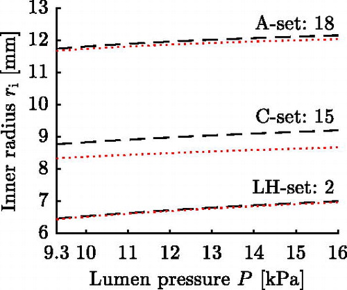
For the generation of data sets, in silico arteries are created using structural and material parameters from the literature. More than one set of structural and HGO material parameters in a publication is rarely found. An exception is the study by Horný et al. (2014), which used data published in Labrosse et al. (2013) to fit the HGO material parameters for 17 human AAs. All reported parameter sets in Horný et al. (2014) are used in this study to create in silico arteries. Out of these, nine sets possess a significantly ($p=0.01$) lower value for parameter c compared to the remaining eight sets. In order to analyze possible implications, the 17 parameter sets are divided into the regular LH-sets (Labrosse/Horný) and the C-sets (low value for parameter c).

The referential radii and axial deformations due to closing of the arterial segments are computed for all 17 sets to guarantee a volume preserving deformation. The values for the same parameters given in Horný et al. (2014) introduce a small violation of this condition and are replaced for the values calculated from Eq. (A1)(A1a) $${\rho }_{\mathrm{i}}=\left({\mathit{R}}_{\mathrm{i}}+\frac{\mathit{H}}{2}\right){\left(1-\frac{{\Phi }_0}{\pi }\right)}^{-1}-\frac{\mathit{H}}{2},$$(A1a) in Appendix A.

The opening angles ${\Phi }_0$ reported in Labrosse et al. (2013) will not, in general, lead to a uniform transmural circumferential strain distribution at MAP (Takamizawa and Hayashi 1987) for the chosen single layer arterial model. To also include in silico AAs respecting a uniform transmural strain distribution and to enlarge the parameter range, five additional parameter sets are created. These five sets respect the uniform strain hypothesis at $\overline{P}=13.3 \text{kPa}$. Figure 2 shows exemplarily the circumferential stretch for three characteristic pressures for a thick-walled FE representation of set 18, cf. Section 3.3.

The parameter sets are summarized in Table 1. Those taken from Labrosse et al. (2013) and Horný et al. (2014) are numbered from 1-8 (LH-sets) and from 9-17 (C-sets). The naming convention introduced in Horný et al. (2014) is given in parenthesis to facilitate comparison. The five additional sets are numbered from 18-22 and will be referred to as A-sets (artificial).

Table 1. Parameter sets representing the created in silico arteries. The regular LH-sets, numbered 1–8, and the C-sets, numbered 9–17, are taken from Labrosse et al. (2013) and Horný et al. (2014). The set numbers within brackets refer to the naming convention in Horný et al. (2014). The sets numbered 18–22 are the artificial A-sets. Note that the reduced axial force ${\widehat{F}}_{\text{red}}$ is stated as its mean value of the corresponding thick-walled FE model.

		Labrosse et al. (2013)			Horný et al. (2014)				Computed		Agreement
		$R_{\mathrm{i}}$	H	${\Phi }_0$	c	k1	k2	β	λz	${\widehat{F}}_{\text{red}}$	$R^2$	RMSE
	Set	[mm]	[mm]	[deg]	[kPa]	[kPa]	[-]	[deg]	[-]	[N]	[-]	[mm]
LH-sets	1 (F49)	5.9	1.51	252.00	2.31	20.06	4.11	39.95	1.1699	0.57	0.63	0.08
	2 (F63)	5.4	0.96	96.00	13.59	41.78	3.29	39.86	1.1594	0.74	0.97	0.03
	3 (M38)	5.3	1.22	117.00	12.20	19.28	3.22	41.60	1.1576	0.74	0.88	0.06
	4 (M60)	6.3	1.69	156.00	5.91	17.57	3.18	43.16	1.1217	0.83	0.72	0.10
	5 (M61b)	7.3	1.62	335.00	6.98	11.37	8.05	41.95	1.1039	0.67	0.52	0.07
	6 (M66)	7.2	1.78	253.00	17.78	25.72	7.65	38.85	1.1385	1.49	0.90	0.04
	7 (M70a)	7.1	1.23	208.00	2.78	67.45	7.02	35.49	1.1908	0.60	0.95	0.03
	8 (M70b)	7.4	1.64	201.00	12.18	17.31	22.86	39.69	1.0582	0.52	0.53	0.05
C-sets	9 (F50)	6.7	1.14	323.00	0.68	49.54	7.44	36.67	1.1791	0.41	0	4.27
	10 (F65)	6.2	1.21	248.00	0.05	9.06	5.87	39.36	1.1932	0.36	0	0.76
	11 (M42)	6.5	1.56	125.00	0.22	21.88	0.62	38.34	1.4322	1.52	0.93	0.09
	12 (M57)	7.5	1.28	322.00	0.05	4.37	4.87	41.11	1.2080	0.55	0	0.61
	13 (M61a)	7.7	1.22	270.00	0.05	49.45	26.74	37.55	1.0836	0.25	0	0.73
	14 (M67a)	8.0	1.58	118.00	0.05	41.95	22.00	38.18	1.0666	0.34	0	1.54
	15 (M67b)	7.9	1.26	174.00	0.05	61.02	7.02	35.49	1.1984	0.56	0	0.49
	16 (M71)	10.0	1.72	118.00	0.05	94.49	9.26	37.65	1.0964	0.84	0	0.70
	17 (M77)	7.0	1.50	135.00	0.05	26.65	39.30	38.23	1.0500	0.19	0	1.39
A-sets	18	10.1	2.81	46.19	32.68	7.44	47.90	40.02	1.0210	0.65	0.34	0.10
	19	14.9	2.81	52.23	67.39	22.53	11.79	47.47	1.0489	5.95	1.0	0.03
	20	5.3	1.41	20.98	75.91	71.16	67.08	37.06	1.0422	1.03	0.96	0.01
	21	3.9	0.68	28.81	90.87	64.35	38.12	39.34	1.0281	0.29	0.99	0.00
	22	12.3	3.54	81.75	28.89	21.33	3.29	53.24	1.0372	3.18	0.98	0.12

3.2. Verification pressure-radius data from thin-walled FE simulation

The verification pressure-radius data sets are created to study if the PI is able to identify the correct parameters when the in silico arteries are consistent with the approximations and assumptions of the mechanical model in Section 2.2. For this reason the verification pressure-radius data sets are generated with thin-walled FE models that do not account for residual stress. Furthermore, the verification data sets also include the time-resolved reduced axial force necessary to keep the in silico AAs at a fixed length.

For each of the 22 parameter sets introduced in Section 3.1, a thin-walled FE model is created using the structural and material parameters summarized in Table 1. The stated opening angles are not used, since residual stress is neglected. Each model is created as a cylinder with mean radius $R_{\mathrm{m}}=R_{\mathrm{i}}+0.5H$ and an arbitrary length L set to 1 mm. This corresponds to using ${\mathcal{B}}^{*}$ in Figure 1 as the stress-free reference configuration. Symmetry in the geometry and for the loading is utilized and therefore only one quarter of the AA is modeled. Four-noded shell elements with a reduced integration scheme (S4R) are selected for the mesh which consists of 100 elements in circumferential direction and 10 elements in the axial direction, see Figure 3a. A thickness H is applied to all elements and a Gauss quadrature with five integration points through the thickness is used.

The simulation is performed with the FE solver Abaqus (Standard version 6.12-3) and involves axial prestretching of the in silico AA followed by pressurization. The employed axial prestretch is stated for each parameter set in Table 1 and its calculation will be explained in Section 3.3. Lumen pressures ranging from 9.3 kPa (70 mmHg) in diastole to 16 kPa (120 mmHg) in systole are chosen for the cardiac cycle (Smoljkić et al. 2015). The values are within the normotensive range (Sonesson et al. 1994).

The cardiac cycle is uniformly divided into $n=101$ pressure levels. For each level the applied pressure P, the inner radius $r_{\mathrm{i}}$, the wall thickness h and the reduced axial force $F_{\text{red}}$ are extracted from the quasi-static FE simulation to serve as a verification pressure-radius data set.

3.3. Validation pressure-radius data from thick-walled FE simulation

The validation pressure-radius data sets are created with in silico arteries capturing experimentally observed AA characteristics. For this reason the validation pressure-radius data sets are generated with thick-walled FE models that account for residual stress.

For each of the 22 parameter sets introduced in Section 3.1, a thick-walled FE model is created using the structural and material parameters summarized in Table 1. Each model is created as a cylindrical sector with an opening angle ${\Phi }_0$, inner radius ${\rho }_{\mathrm{i}}$, outer radius ${\rho }_{\mathrm{o}}$ and an arbitrary length ζ set to 1 mm. This corresponds to using ${\mathcal{B}}_0$, cf. Figure 1, as the stress-free reference configuration. Symmetry in the geometry and for the loading is utilized and therefore only one half of the AA is modeled. Eight-noded brick elements based on a mixed formulation (C3D8H) are selected for the mesh which consists of 200 elements in circumferential direction and 10 elements in both the radial and the axial direction, see Figure 3b.

The simulation is divided into two stages: closing and loading. In the closing stage, the cut-open circular sector is closed to form a tube, see algorithm in Appendix A. In the loading stage, the in silico AA is prestretched and afterwards pressurized in the range of 9.3 kPa to 16 kPa representing the cardiac cycle, cf. Section 3.2. The magnitude of the employed axial prestretch is chosen such that for the respective in silico AA the reduced axial force $F_{\text{red}}$ is approximately constant throughout the cardiac cycle (Van Loon et al. 1977; Weizsäcker et al. 1983; Schulze-Bauer et al. 2003). The in situ axial prestretch λ_z is determined in an iterative process in which the prestrech is altered until the above condition is fulfilled. Figure 4 shows the result of this process for set 18, and for all parameter sets the determined in situ axial prestretch λ_z and mean reduced axial force ${\widehat{F}}_{\text{red}}$ are stated in Table 1. Once the in situ axial prestretch is determined, the pressure-radius curve is ocularly inspected to make sure it shows the exponential shape typically observed for arteries (Roach and Burton 1957).

The stage corresponding to the cardiac cycle of the simulation is uniformly divided into $n=101$ pressure levels. For each level the applied pressure P, the inner radius $r_{\mathrm{i}}$ and the wall thickness h are extracted from the quasi-static FE simulation to serve as a validation pressure-radius data set.

4. Parameter identification method

The idea behind the PI is to calculate two sets of stresses for a given pressure-radius data set and determine the model parameters by a non-linear least squares fitting of the stresses (Schulze-Bauer and Holzapfel 2003). The first set is the equilibrium stresses computed using the Laplace laws in Eq. (18)(18a) $${\sigma }_{\theta \theta }^{\text{Lp}}=\left(\frac{r_{\mathrm{i}}}{h}+\frac{1}{2}\right)P,$$(18a) , while the second set is the constitutively determined stresses in Eq. (22)(22a) $$\begin{array}{c}{\sigma }_{\theta \theta }^{\text{mod}}=2c[{\lambda }_{\theta ,\mathrm{m}}^2-{\left({\lambda }_{\theta ,\mathrm{m}}{\lambda }_z\right)}^{-2}]+\hfill \\ 4k_1\left(I_4-1\right){\mathrm{e}}^{k_2{\left(I_4-1\right)}^2}{\lambda }_{\theta ,\mathrm{m}}^2{\hspace{0.17em}\text{cos}\hspace{0.17em}}^2\beta ,\hfill \end{array}$$(22a) .

4.1. Error function

The error function ε is defined as a weighted sum between the squared errors of the two sets of stresses, i.e. (23) $$\begin{array}{c}\epsilon \left(\mathit{\kappa }\right)=\sum _{j=1}^n\{w{[{\sigma }_{\theta \theta }^{\text{mod}}\left(\mathit{\kappa },r_{\mathrm{i},j}\right)-{\sigma }_{\theta \theta }^{\text{Lp}}\left(r_{\mathrm{i},j},P_j\right)]}^2\hfill \\ +\left(1-w\right){[{\sigma }_{zz}^{\text{mod}}\left(\mathit{\kappa },r_{\mathrm{i},j}\right)-{\sigma }_{zz}^{\text{Lp}}\left(r_{\mathrm{i},j},P_j\right)]}^2\},\hfill \end{array}$$(23) where $\mathit{\kappa }=(R_{\mathrm{i}}, {\lambda }_z, c, k_1, k_2, \beta )$ is the parameter vector, the index j denotes a data point, n is the total number of data points and $w\in \left[0,1\right]$ is a weighting factor. The weighing factor is set to $w=0.99$ in order to let the error function be dominated by the circumferential part, see Discussion. The PI problem reads: $$\{\begin{array}{c}\underset{\mathit{\kappa }\in {\mathbb{R}}^6}{\min }\epsilon \left(\mathit{\kappa }\right)\hfill \\ \text{subject} \text{to}: {\mathit{\kappa }}_{\text{min}}\le \mathit{\kappa }\le {\mathit{\kappa }}_{\text{max}},\hfill \end{array}\left(\mathbf{P}\right)$$ where ${\mathit{\kappa }}_{\text{min}}$ and ${\mathit{\kappa }}_{\text{max}}$ denote the lower and upper bounds on $\mathit{\kappa }$, respectively. The minimization fitting ranges, see Table 2, are based on experimental observations and chosen such that they do not become active during the minimization. For parameter λ_z the lower limit is set to 1.0 to avoid buckling.

Table 2. Fitting ranges of the structural and material parameters of the AA.

Parameter	$R_{\mathrm{i}}$	λz	c	k1	k2	β
	[mm]	[-]	[kPa]	[kPa]	[-]	[deg]
${\mathit{\kappa }}_{\text{min}}$	0.1	1	$1·{10}^{-7}$	$1·{10}^{-7}$	$1·{10}^{-4}$	0
${\mathit{\kappa }}_{\text{max}}$	25	10	$3·{10}^3$	$6·{10}^3$	$4·{10}^3$	90

4.2. Implementation

The PI problem in ($\mathbf{P}$) is well-posed, but non-linear and non-convex. Such problems typically possess local solutions that are not global solutions (Nocedal and Wright 1999). To circumvent this issue, we use a local search method with multiple starting points. The local solution that has the lowest error function value is assumed to be the global optimum.

The PI problem is solved in Matlab R2015a (The MathWorks Inc., Natick, MA, USA) using the function fmincon with the interior-point optimization algorithm. For numerical efficiency the parameters c, k₁, k₂ and β are replaced by scaled counterparts to make the minimization more balanced (Nocedal and Wright 1999), (24) $$c={\mathrm{e}}^{\tilde{c}},\hspace{1em}{k}_1={\mathrm{e}}^{{\tilde{k}}_1},\hspace{1em}{k}_2={\mathrm{e}}^{{\tilde{k}}_2},\hspace{1em}\beta =\arcsin \tilde{\beta },$$(24) where the superscribed tilde indicates a scaled parameter. The analytical gradient and Hessian of the error function in Eq. (23)(23) $$\begin{array}{c}\epsilon \left(\mathit{\kappa }\right)=\sum _{j=1}^n\{w{[{\sigma }_{\theta \theta }^{\text{mod}}\left(\mathit{\kappa },r_{\mathrm{i},j}\right)-{\sigma }_{\theta \theta }^{\text{Lp}}\left(r_{\mathrm{i},j},P_j\right)]}^2\hfill \\ +\left(1-w\right){[{\sigma }_{zz}^{\text{mod}}\left(\mathit{\kappa },r_{\mathrm{i},j}\right)-{\sigma }_{zz}^{\text{Lp}}\left(r_{\mathrm{i},j},P_j\right)]}^2\},\hfill \end{array}$$(23) are computed using Maple 2015.1 (Maplesoft, Waterloo, Ontario) and provided to fmincon to facilitate the minimization. An optimization run is deemed successful if the absolute change of each member of $\mathit{\kappa }$ between consecutive iterations is less than ${10}^{-10}$ and if the absolute change of the error function ε is less than ${10}^{-6}$.

The starting points are generated by defining a MultiStart class in Matlab. Initially 100 starting points are distributed over the entire parameter space using Latin Hypercube Sampling (Myers et al. 2009). Starting points predicting unrealistic model stresses are dropped and the procedure is repeated with a progressively increasing number of starting points, until at least 100 starting points predict stress values in the interval $0.0 \text{kPa}<{\sigma }_{\theta \theta }^{\text{mod}},{\sigma }_{zz}^{\text{mod}}<{10}^5 \text{kPa}$. These limits are based on reported stress values for human arteries (Gasser et al. 2002; Labrosse et al. 2013; Holzapfel and Ogden 2015).

5. Results

The results section is divided into two parts. First the PI is verified using the verification data sets (Section 3.2). Then the PI is validated using the validation data sets generated with in vivo-like AAs (Section 3.3).

In what follows, identified parameters are indicated by the superscript Id while the exact (pre-defined) values used in the corresponding FE simulations are indicated by the superscript FE. Data points corresponding to the LH-sets are displayed using a red asterisk, the A-sets are represented by red diamonds and for the C-sets blue squares are chosen. The results show that the difference between the identified and pre-defined parameters is much larger for the C-sets, see Tables 3 and 4. The figures are, therefore, adjusted to display the results of the LH- and A-sets. Mean differences and 95% limits of agreement are displayed only for the LH-sets and A-sets.

Table 3. Mean difference and 95% limits of agreement of identified and FE values for the verification.

		LH- and A-sets		C-sets
Parameter	Unit	Mean difference	95% limits of agreement	Mean difference	95% limits of agreement
$R_{\mathrm{i}}$	[mm]	0.002	–0.007 to 0.011	0.25	–1.01 to 1.53
λz	[-]	–0.001	–0.002 to 0.001	0.51	–1.53 to 2.54
c	[kPa]	0.034	–0.017 to 0.085	0.02	–0.07 to 0.11
k1	[kPa]	0.075	–0.110 to 0.259	0.67	–0.23 to 1.57
k2	[-]	0.026	–0.043 to 0.094	0.13	–0.13 to 0.46
β	[deg]	0.008	–0.049 to 0.065	–5.67	–30.14 to 18.80

Table 4. Mean difference and 95% limits of agreement of identified and FE values for the validation.

		LH- and A-sets		C-sets
Parameter	Unit	Mean difference	95% limits of agreement	Mean difference	95% limits of agreement
$R_{\mathrm{i}}$	[mm]	0.09	–0.34 to 0.52	0.14	–1.27 to 1.55
λz	[-]	0.04	–0.13 to 0.20	2.50	–0.42 to 5.41
c	[kPa]	0.36	–1.80 to 2.51	0.99	–2.29 to 4.27
k1	[kPa]	–0.01	–10.23 to 10.21	3.68	–24.69 to 32.05
k2	[-]	0.98*	0.75 to 1.21*	1.10*	0.41 to 1.78*
β	[deg]	–3.80	–9.97 to 2.37	–22.56	–51.87 to 6.76

*Mean ratio and the corresponding 95% limits of agreement are presented instead.

5.1. Verification

The PI is verified using the 22 data sets described in Section 3.2. Since the correct reduced axial force $F_{\text{red}}$ is included in these data sets, it is used in the PI. This means that ${\overline{F}}_{\text{red}}$ in Eq. (18(18a) $${\sigma }_{\theta \theta }^{\text{Lp}}=\left(\frac{r_{\mathrm{i}}}{h}+\frac{1}{2}\right)P,$$(18a) b) is replaced by $F_{\text{red}}$ for the verification. On average 62% of the starting points converge to the (assumed) global optimum for the LH- and A-sets. For the C-sets significantly fewer starting points converge, on average 6%. For sets 10 and 12 the error function is unaffected by changes in parameter c and the Hessian lost its rank at the solution, thus suggesting a non-unique solution.

To assess the agreement between identified and pre-defined parameters, a Bland-Altman plot (Bland and Altman 1999) is created for each parameter in which the differences between the identified and the FE values are plotted against the FE values, see Figure 5. In addition, the mean differences and 95% limits of agreement are summarized in Table 3. In case of the LH- and the A-sets the differences are very small, both indicated by a low mean difference and narrow 95% limits of agreement for each parameter. Furthermore, no systematic error, which would be expressed by a correlation between the differences and the FE values, is evident. For the C-sets larger differences occur, indicated by the non-displayed data points in Figure 5 and the calculated mean differences and 95% limits of agreement in Table 3.

5.2. Validation

After verifying the PI, it is validated using the validation pressure-radius data generated with in vivo-like AAs, cf. Section 3.3. The average time for identifying the model parameters for one pressure-radius data set is 39 min on a quad core 2.3 GHz CPU. On average 59% of the starting points converge to the (assumed) global optimum for the LH-sets and the A-sets. For the C-sets, significantly fewer starting points, on average 5%, converge to the same solution. For sets 12, 13 and 14 the error function is unaffected by changes in parameter c and the Hessian lost its rank at the solution. For set 11 an axial prestretch of ${\lambda }_z=1.0$ is identified, i.e. the lower boundary for this parameter is reached.

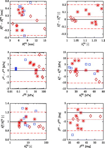
Bland-Altman plots are created for each parameter, see Figure 6. For parameter k₂ the differences between identified and pre-defined values increase as the pre-defined values increase. To compensate for this systematic error, the ratios of identified and pre-defined values are plotted against the FE values instead (Eksborg 1981; Bland and Altman 1999).

For the LH- and the A-sets, the agreement for parameters $R_{\mathrm{i}}$ and c is high, indicated by a low mean difference and narrow 95% limits of agreement, see Table 4. Parameter k₁ exhibits a vanishingly small mean difference, but the limits of agreement are wide compared to $k_1^{\text{FE}}$. Similar to k₁, parameter k₂ shows a small mean difference, expressed by a mean ratio of 0.98, but identified values are estimated to be between 21% too large and 25% too small. The angle β is underestimated by almost $4°$ on average and the 95% limits of agreement are $-9.97°$ and $2.37°$, respectively. The largest percentage discrepancies are seen for λ_z.

For every parameter of the C-sets the mean difference is larger and the 95% limits of agreement are wider compared to the LH- and A-sets. This is especially true for parameters λ_z and β. For sets 10 and 12-17 axial prestretches of ${\lambda }_z>4.0$ and angles of $\beta <10°$ are identified. For sets 9 and 11, the remaining two members of the C-sets, axial prestretches of 1.6 and 1.0 and somewhat reasonable values for β are identified.

6. Discussion

In this study, a numerical technique is used to both verify and validate an in vivo PI. The same limitations as discussed in Smoljkić et al. (2015), who proposed the chosen validation procedure, apply. This numerical investigation is not a replacement for an experimental validation, in which the identified parameters would be compared to the results of e.g. in vitro inflation-extension tests. The choice to use a numerical technique allows a straight forward comparison of identified and pre-defined (material) parameters and avoids typical experimental complications. Following this numerical validation an experimental validation is to be conducted.

6.1. Generation of in silico data

The in silico arteries used for validation are created with emphasis on capturing the arterial response observed in in vitro experiments. The thick-walled FE model takes the thick-walled nature of arteries into account together with its composition of an isotropic matrix with embedded collagen fibers (Holzapfel et al. 2000). Residual stress is introduced using the opening angle method (Chuong and Fung 1986). For the A-sets, the opening angle is chosen to respect the uniform strain hypothesis at MAP (Takamizawa and Hayashi 1987). Furthermore, the applied axial prestretch is chosen such that the reduced axial force is approximately constant throughout the cardiac cycle (Van Loon et al. 1977; Weizsäcker et al. 1983; Schulze-Bauer et al. 2003). To limit the scope of the present study and to enable a straightforward comparison with the in vivo PI, certain characteristics of an artery are excluded. The utilized FE models are based on a perfectly cylindrical, homogeneous arterial wall. In reality, the tissue is substantially more complex. The assumption of a perfectly shaped cylinder is chosen for simplicity and no adequate data has been found in the literature to account for possible eccentricity of an AA during the cardiac cycle. The effect of non-uniform wall thickness (Li et al. 2004; Holzapfel et al. 2007; Sokolis et al. 2017) on the PI is unknown. This limitation is believed to be of minor importance, however. In Ferraro et al. (2018) it is shown that the deformation fields of a uniform and a non-uniform thickness FE model are very similar in bifurcation free regions. The arterial wall also consists of two to three distinct layers with different mechanical properties (Holzapfel et al. 2007; Rhodin 2014). Multi-layered structures are dropped to allow for a straightforward comparison of identified and pre-defined parameters. The parameter sets in Table 1 are, therefore, thought of representing the global response of the individual layers.

In addition, an artery is not solely subjected to luminal pressure in vivo but constrained in its radial deformation by surrounding tissue, organs and bones (Boutouyrie et al. 1997). Hence, the assumption of zero traction on the outside of the artery in Section 2.1.3 does not hold. The surrounding of an artery could be modeled (Kim et al. 2013), but typically an axisymmetric pressure is applied to the outside of the arterial wall to account for the perivascular state (Singh and Devi 1990; Humphrey and Na 2002; Masson et al. 2008; Wittek et al. 2016). No information about the perivascular state is reported in Labrosse et al. (2013). Singh and Devi (1990) investigated the influence of perivascular pressure and it appears to be very small. The outer boundary of an artery is therefore chosen to be traction free.

Another limitation is the negligence of the active contribution of smooth muscle cells. They have a profound effect on small arteries (Cox 1978), but are of minor importance for the aorta (Sonesson et al. 1997; Dobrin 2011) and it is therefore a reasonable assumption to neglect smooth muscle activity in case of the AA.

To the best of the authors’ knowledge, only the study by Horný et al. (2014) reports both geometrical and HGO material parameters suitable for this validation. The stated values for parameter c are very low for the C-sets. As a consequence the isotropic material stores less than 2% of the total strain energy in the vessel wall for these in silico AAs. This is not the expected behavior of healthy arteries (Roach and Burton 1957). Such low c parameters have only been reported for the elderly and for abdominal aortic aneurysms (Ferruzzi et al. 2011). Although Labrosse et al. (2013) excluded pathological aortic samples from their study, these AAs may have experienced age or pathology related micro-structural changes not observable through ocular inspection.

The in situ axial prestretches of the AAs are not stated by Labrosse et al. (2013) and needed to be determined. The calculated values for the LH- and the C-sets agree with experimental measurements except for set 11 (Langewouters et al. 1984; Horný et al. 2011). The determined in situ axial prestretch ${\lambda }_z\approx 1.43$ for this set is very high compared to previously reported values for this age group (Langewouters et al. 1984; Schulze-Bauer et al. 2003; Horný et al. 2011). Nevertheless, this parameter set is included to study the robustness of the method for extreme values. The determined in situ axial prestretches for the A-sets are physiological and coincide with values for the elderly (Horný et al. 2011). The high reduced axial forces for both sets 19 and 22 exceed what has been reported previously for human arteries (Schulze-Bauer et al. 2003) and other species (Takamizawa and Hayashi 1987; Weizsäcker and Kampp 1990). Again, these parameter sets are kept to study the robustness of the method for extreme values.

The decision to use the HGO model for generation of the in silico data is made to allow a direct comparison of the FE parameters and those identified by the PI. More sophisticated constitutive models based on the HGO model are available which offer similar parameters, although not directly comparable. In the study by Gasser et al. (2006), the HGO model is generalized to account for a distribution of the collagen fibers by introducing a parameter κ. In recent years this model has been utilized in many studies (Haskett et al. 2010; Weisbecker et al. 2012; Horný et al. 2014; Smoljkić et al. 2015; Wittek et al. 2016). Its common implementation for excluding compressed collagen fibers has been questioned, however (Holzapfel et al. 2015). Experimentally derived parameter sets based on the material model proposed in Gasser et al. (2006) are therefore not used herein. A recent material model proposed in Holzapfel and Ogden (2015) accounts for non-symmetric collagen fiber dispersion, but due to its novelty not sufficiently many parameter sets have been found in the literature.

6.2. Limitations of the in vivo parameter identification method

The artery is modeled as a thin-walled cylinder in the PI. Although this assumption is questionable from a physiological point of view, it helps to reduce the non-convexity of the minimization problem considerably compared to treating the artery as a thick-walled cylinder. Smoljkić et al. (2015) address this issue by introducing three assumptions related to the physiological behavior of arteries. Their first assumption is that the reduced axial force is approximately constant throughout the cardiac cycle. This has been observed experimentally (Van Loon et al. 1977; Weizsäcker et al. 1983; Schulze-Bauer et al. 2003) and also been successfully used before to improve a PI (Stålhand and Klarbring 2005). Their second condition attempts to equalize the strain-energy across the arterial wall in order to reduce the stress gradient. Smoljkić et al. (2015) do not introduce a residual stress field, however, and a uniform strain-energy or stress across the wall at non-zero pressure is impossible in that case (Rachev and Hayashi 1999). Hence, a solution to the minimization problem fulfilling the second condition proposed in Smoljkić et al. (2015) does not exist. The third condition stating that at diastolic pressure the matrix material and the collagen fibers store approximately the same amount of strain-energy has only been shown for the AA of rat (Smoljkić et al. 2015) and not been confirmed for human arteries. When evaluating the strain-energy stored in the collagen fibers at diastolic pressure for all generated in silico AAs, it varies between 50-91% of the total strain-energy for the LH-sets, between 12-25% for the A-sets and between 98-100% for the C-sets. Hence the statement that elastin and collagen store the same amount of strain-energy seems to be questionable for human AA based on this study.

The approach suggested in Smoljkić et al. (2015) imposes questionable assumptions to obtain a unique set of parameters when treating an artery as a thick-walled cylinder. As shown by the validation herein, treating the human AA as a thin-walled cylinder is sufficient to determine the referential radius and the mechanical properties of the collagen fibers and the non-collagenous material over a large range of values, at least, for the LH- and A-sets. For the C-sets, the proposed PI does not identify acceptable parameters. This is accompanied by a low percentage of converging starting points, rank degradation of the Hessian at the solution and/or parameters reaching the parameter boundary.

To get a better understanding of how the identified parameters represent the in silico AAs, the identified parameters are used to create thick-walled FE models. These models are constructed as described in Section 3.3 with the difference that residual stress is neglected $\left({\Phi }_0^{\text{Id}}=0\right)$ and that the identified axial prestretch ${\lambda }_z^{\text{Id}}$ is applied. From the cardiac cycle the applied pressure P and the inner radius $r_{\mathrm{i}}^{\text{Id}}$ are extracted and compared to the pressure-radius curve of the respective in silico AA (validation pressure-radius data set). To quantify the agreement between two pressure-radius curves, the coefficient of determination R² and the root-mean-square error RMSE are calculated. The calculated coefficient of determination and root-mean-square error are stated in Table 1 for each set. The R² values are notably lower for the C-sets and even negative in some cases indicating a complete inability to represent the data (Kvalseth 1985). In these cases, R² is set to zero for easy interpretation. Figure 7 shows the pressure-radius response for the simulated in silico artery together with the predicted response using the identified parameters for three representative sets. The identified deformation behavior is in close agreement for the LH- and A-sets, which is also confirmed by the R² and RMSE values in Table 1. In fact, there is almost no visual difference between predicted and validation pressure-radius data among the LH- and A-sets, compare sets 2 and 18 in Figure 7. For the C-sets with the exception of set 11 large discrepancies occur, however. In Figure 7 the pressure-radius curves are compared for Set 15, which after set 11 has the lowest RMSE value among the C-sets, and the discrepancy is notable.

In order to compensate for the lack of axial information in the in vivo measurable data of an artery, i.e. the axial prestretch and the reduced axial force, the assumption is made that the ratio between the axial and circumferential stress is known for the MAP pressure (Schulze-Bauer and Holzapfel 2003). As shown by Smoljkić et al. (2015), this ratio may differ from $\gamma =0.59$ and using an incorrect value results in poor parameter estimates. When calculating the ratio γ for all generated in silico AAs it varies between 0.50-0.64 for the LH-sets between 0.45-0.71 for the A-sets and between 0.45-0.65 for the C-sets. The axial to circumferential stress ratio varies but the interval includes the used value. As a consequence the axial equilibrium stress in Eq. (18(18a) $${\sigma }_{\theta \theta }^{\text{Lp}}=\left(\frac{r_{\mathrm{i}}}{h}+\frac{1}{2}\right)P,$$(18a) b) and therefore the axial model stress in Eq. (22(22a) $$\begin{array}{c}{\sigma }_{\theta \theta }^{\text{mod}}=2c[{\lambda }_{\theta ,\mathrm{m}}^2-{\left({\lambda }_{\theta ,\mathrm{m}}{\lambda }_z\right)}^{-2}]+\hfill \\ 4k_1\left(I_4-1\right){\mathrm{e}}^{k_2{\left(I_4-1\right)}^2}{\lambda }_{\theta ,\mathrm{m}}^2{\hspace{0.17em}\text{cos}\hspace{0.17em}}^2\beta ,\hfill \end{array}$$(22a) b) are incorrectly estimated. The axial model stress is most sensitive to parameter λ_z, which is in turn also incorrectly estimated. To address the selected incorrect ratio γ and subsequent erroneously determined reduced axial force a weighing factor w is introduced in the error function (23). This weighing factor is set so that the error function is dominated by the circumferential part. A small influence $\left(1\%\right)$ of the axial stress has a positive effect on the PI, however.

In this context we have attempted to, on the one hand, completely remove the axial component from the error function while, on the other hand, introduce the reduced axial force as an additional unknown parameter to the optimization problem. In both cases the Hessian loses its rank at the solution, suggesting a non-unique solution, and the identified parameters are poor.

An alternative approach is to remove the axial prestretch λ_z as a parameter to be identified but specify it instead. Horný et al. (2011) found a correlation between age and axial prestretch λ_z for the male AA. This approach is very appealing, but the PI aims to be applicable for both sexes, other arteries and other species as well. Hence, the more general approach based on an approximately constant reduced axial force throughout the cardiac cycle is used until such data is available for both sexes, other arteries and other species. Nevertheless, the data provided by Horný et al. (2011) for λ_z and other research groups for the remaining model parameters could be included in the PI by means of a Bayesian approach (Kennedy and O’Hagan 2001; Seyedsalehi et al. 2015).

Another limitation of the proposed PI is the choice of the constitutive model. As discussed, more recent material models, that incorporate e.g. fiber dispersion (Gasser et al. 2006; Holzapfel and Ogden 2015), are available to describe arterial tissue. However, already by introducing one further unknown parameter non-uniqueness becomes a problem in the PI. In addition, the HGO material model is developed for healthy tissue and does not account for smooth muscle activity. While smooth muscle activity is of minor importance in the aorta (Sonesson et al. 1997; Dobrin 2011), the influence of disease needs to be addressed in the future before the method can be used in e.g. a clinical environment.

With respect to the implementation of the PI, one aspect requires further attention. As stated in Section 4.2 the minimization problem in ($\mathbf{P}$) is non-convex and such problems typically possess local solutions that are not global solutions. In this study this aspect was addressed by using a local search method with multiple starting points. For all 22 in silico AAs several local solutions were found and the one with the lowest error function value was taken to be the global one. As indicated by the high amount of starting points converging to the same solution for both the LH- and the A-sets, it is reasonable to assume that the global solution has been identified. This was further corroborated by a test in which the amount of starting points was increased by a factor ten without changing the solution. For the C-sets only a few starting points ended up in the same solution with the lowest error function value. Additionally, for sets 12, 13 and 14 sets the Hessian loses its rank at the solution, thus suggesting a non-unique solution, and for set 11 the boundary was reached. Thus, it is unlikely that the global solution was obtained for either of those pressure-radius data sets. The difficulty of identifying the global solution for the C-sets is associated with the extremely low value for parameter c and the resulting negligible isotropic response of the in silico AAs. Although the PI predicts correctly the diminishing isotropic response, the identified parameters are incorrect, because all parameters but c can then only be identified with respect to the anisotropic response. Increasing the number of starting points by a factor 100 did not improve the result for the C-sets. An interesting venue for future research is to consider more systematic methods for global optimization (Neumaier 2004) to make sure that global solutions are obtained.

7. Conclusion

In this study, an in vivo PI for arteries is further developed and numerically both verified and validated for the human abdominal aorta. For the validation, 22 in silico pressure-radius data sets are generated using the FE method and pre-defined parameters based on the human AA. The identified parameters are in good agreement with the pre-defined ones, especially for the referential radius and the material constant associated with elastin. Only the in situ axial prestretch is incorrectly identified. For pathological AAs erroneous parameters are identified, but the PI exposes such aortas.

The usage of 22 in silico AAs for the validation demonstrates not only the robustness of the presented PI, but also gives valuable insight into its accuracy.

Disclosure statement

No potential conflict of interest was reported by the authors.

Figure 7. Comparison of predicted (red dotted line) with validation pressure-radius data (black dashed line) for parameter sets 2, 15 and 18 from Table 1.

Additional information

Funding

This work was supported by the Swedish Research Council [grant number 621-2014-4165].

Appendix A. Accounting for residual stress in arteries

In this appendix we briefly describe how to account for residual stresses in a FE simulation. The fundamental assumption is that one radial cut through an intact ring-shaped arterial segment fully releases the residual stress, cf. Section 2.1.1. The resulting stress-free geometry is described by a cylindrical segment with an opening angle ${\Phi }_0$, cf. Figures 1 and A1. By modeling this cylindrical segment and closing it to form a cylinder, one accounts for residual stresses in the FE model. Similar procedures are described in the literature (Gasser et al. 2002; Balzani et al. 2007; Famaey et al. 2012), but they are only applicable for fairly low opening angles and do not work for values above ${\Phi }_0>\pi$. Many arteries exhibit high opening angles (Saini et al. 1995; Okamoto et al. 2002; Holzapfel et al. 2007; Labrosse et al. 2013; Sokolis et al. 2017) and there is a need for a procedure that is able to compute residual stress in such arteries, which has not been documented to the best of the authors’ knowledge. The following procedure is both applicable for ${\Phi }_0<\pi$ and ${\Phi }_0>\pi$.

The procedure used herein assumes the artery to be a perfectly cylindrical segment. The unloaded inner radius ${\mathit{R}}_{\mathrm{i}}$ and thickness H are given, cf. Section 3, but their referential equivalents need to be determined for creating the thick-walled FE model. For this purpose it is assumed that in addition to $\mathit{L}=\zeta$, cf. Section 2.1.1, the arterial wall will not change its thickness throughout the closing process, i.e. $\mathit{H}=\eta$ (Labrosse et al. 2013). By enforcing incompressibility the referential radii are then calculated as (A1a) $${\rho }_{\mathrm{i}}=\left({\mathit{R}}_{\mathrm{i}}+\frac{\mathit{H}}{2}\right){\left(1-\frac{{\Phi }_0}{\pi }\right)}^{-1}-\frac{\mathit{H}}{2},$$(A1a) (A1b) $${\rho }_{\mathrm{o}}={\rho }_{\mathrm{i}}+\mathit{H}.$$(A1b)

Note that for opening angles ${\Phi }_0>\pi$ the referential inner ${\rho }_{\mathrm{i}}$ and outer ${\rho }_{\mathrm{o}}$ radii are reversed and exhibit negative values (Labrosse et al. 2013; Horný et al. 2014).

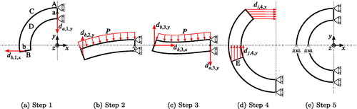
The open arterial segment is sketched in the xy-plane with the origin at (0, 0, 0) as its center and one end of the artery has to be located on the yz-plane, see Figure A1. Depending on whether ${\Phi }_0<\pi$ or ${\Phi }_0>\pi$, the geometry has to be located in the third and partly the second (Figure A1a) or the second and partly the third quadrant (Figure A1b) of the xy-plane, respectively. When extruding the sketch in the z-direction, let the formed surfaces be called A, B, C and D as in Figure A2a. A mesh with an even number of elements in the circumferential direction needs to be defined, so once the arterial segment is closed one set of nodes will lie in the xz-plane. Let this set of nodes be called E, cf. Figure A2d. Two additional nodes a and b need to be created in the middle of their corresponding surfaces A and B, cf. Figure A2a. Between nodes a and b, and their respective surface, a constraint is defined that couples the translation by uniformly distributing the force of the reference node to the coupled nodes. In the following the closing process of the artery is described.

Figure 2. Circumferential stretch for the pressures 9.3, 13.3 and $16 \text{kPa}$ for parameter set 18 from Table 1.

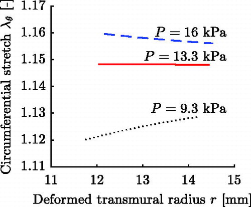
Figure 3. Examples of meshes for two different FE models of an AA.

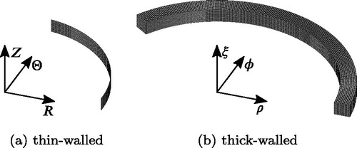
Figure 4. Reduced axial force for three different axial prestretches for parameter set 18 from Table 1.

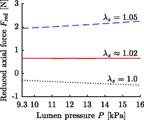
Figure 5. Difference between identified and FE values plotted against the FE values for each parameter of the verification sets. The solid black lines represents perfect agreement, the dotted red line is the mean difference and the dashed red lines denote the 95% limits of agreement of the LH- and A-sets. Note that a logarithmic abscissa is used for parameters c and k₂.

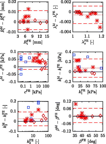
Figure 6. Difference between identified and FE values plotted against the FE values for each parameter of the validation sets. The solid black lines represents perfect agreement, the dotted red line is the mean difference and the dashed red lines denote the 95% limits of agreement of the LH- and A-sets. Note that for parameter k₂ the ordinate shows the ratio of identified and pre-defined value and a logarithmic abscissa is used for parameters c and k₂.

In a first step (Figure A2a) the cylindrical segment is pulled on one side in order to straighten the arterial segment. To this end a displacement ${\mathit{d}}_{\mathit{b},1,\mathit{x}}$ is prescribed to reference node b: (A2) $${\mathit{d}}_{\mathit{b},1,\mathit{x}}=\left(\left|{\rho }_{\mathrm{i}}\right|+\frac{\mathit{H}}{2}\right)\left|{\Phi }_0-\pi \right|+{\mathit{x}}_{\mathit{b}},$$(A2) where x_b is the x-coordinate of node b. Since the center of the closed arterial segment shall be positioned at the origin (0, 0, 0) as in Figure A2e the whole segment needs to be moved. Therefore a displacement ${\mathit{d}}_{\mathit{a},1,\mathit{y}}=-{\rho }_{\mathrm{i}}-\mathit{H}/2$ is applied to node a. Furthermore, the surface A is constrained in x-direction, surface C is constrained in z-direction and the opposing surface D is allowed to move freely in z-direction under the condition that all nodes move the same amount. The allowed z-movement is to enable incompressibility during the closing process. These three surface BCs will continue throughout the entire closing process until further notice.

The second step (Figure A2b) is designed to assure that the arterial segment bulges in the correct way before further closing the artery. Therefore a sufficiently large pressure, typically 1 kPa, at the later to be inner boundary of the artery is applied. This is accompanied by replacing the x-displacement BC of node b to a y-displacement ${\mathit{d}}_{\mathit{b},2,\mathit{y}}=-{\mathit{y}}_{\mathit{b}}$, where y_b is its reference y-coordinate. Node a is further constrained in y-direction.

In the third step (Figure A2c) the arterial segment is almost closed. Both x- and y-displacements are assigned to node b according to (A3a) $${\mathit{d}}_{\mathit{b},3,\mathit{x}}=-\frac{\mathit{H}}{2}-{\mathit{x}}_{\mathit{b}},$$(A3a) (A3b) $${\mathit{d}}_{\mathit{b},3,\mathit{y}}={\mathit{R}}_{\mathrm{i}}+\frac{\mathit{H}}{2}-{\mathit{y}}_{\mathit{b}}.$$(A3b)

Node a is further displaced by ${\mathit{d}}_{\mathit{a},3,\mathit{y}}=-{\rho }_{\mathrm{i}}+{\mathit{R}}_{\mathrm{i}}$.

In the fourth step (Figure A2d) the arterial segment is fully closed and the pressure load is removed. Therefore an individual x-displacement BC is applied to each node line of surface B, where the radial direction is discretized using n node lines starting from i = 1 at the inner boundary and ending at i = n at the outer boundary. The corresponding BCs are (A4) $${\mathit{d}}_{\mathit{i},4,\mathit{x}}=-{\mathit{x}}_{\mathit{i}},\mathit{i}=1,\dots ,\mathit{n},$$(A4) where x_i is the x-coordinate of the ith node line. In addition the node lines of surface E, let them start at j = 1 at the inner and end at j = m at the outer radius, are displaced individually according to (A5) $${\mathit{d}}_{\mathit{j},4,\mathit{y}}=-{\mathit{y}}_{\mathit{j}},\mathit{j}=1,\dots ,\mathit{m},$$(A5) where y_j is the y-coordinate of the jth node line.

The final step (Figure A2e) homogenizes the stress field within the artery. Therefore the displacement constraints of step four are substituted by symmetry BCs, meaning that both planes A and B are only constrained in x-direction and plane E in y-direction. Surface C is still constrained in z-direction and surface D is displaced to its reference position, since no axial deformation due to the closing is assumed (Chuong and Fung 1986).

Figure A1. Example geometries of the arterial segment for different opening angles. For explanation of the parameters see Appendix A.

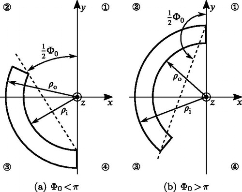
Figure A2. BCs of the different simulation steps illustrated for an artery with ${\Phi }_0>\pi$. For explanation of the parameters see Appendix A.

References

- Åstrand H, Stålhand J, Karlsson J, Karlsson M, Sonesson B, Länne T. 2011. In vivo estimation of the contribution of elastin and collagen to the mechanical properties in the human abdominal aorta: effect of age and sex. J Appl Physiol. 110(1):176–187.
- Balzani D, Schröder J, Gross D. 2007. Numerical simulation of residual stresses in arterial walls. Comput Mater Sci. 39(1):117–123.
- Bland JM, Altman DG. 1999. Measuring agreement in method comparison studies. Stat Methods Med Res. 8(2):135–160.
- Boutouyrie P, Bézie Y, Lacolley P, Challande P, Chamiot-Clerc P, Benetos A, Renaud de la Faverie J, Safar M, Laurent S. 1997. In vivo/in vitro comparison of rat abdominal aorta wall viscosity. Arterioscler Thromb Vasc Biol. 17(7):1346–1355.
- Bramwell JC, Hill AV. 1922. The velocity of the pulse wave in man. Proc R Soc B Biol Sci. 93(652):298–306.
- Burton AC. 1954. Relation of structure to function of the tissues of the wall of blood vessels. Physiol Rev. 34(4):619–642.
- Chuong CJ, Fung YC. 1986. On residual stresses in arteries. J Biomech Eng. 108(2):189–192.
- Cox RH. 1978. Regional variation of series elasticity in canine arterial smooth muscles. Am J Physiol. 234(5):H542–H551.
- Dobrin PB. 2011. Vascular mechanics. Compr Physiol. 3:65–102.
- Dobrin PB, Rovick AA. 1969. Influence of vascular smooth muscle on contractile mechanics and elasticity of arteries. Am J Physiol. 217(6):1644–1651.
- Ecobici M, Stoicescu C. 2017. Arterial stiffness and hypertension - which comes first? Maedica (Buchar)). 12(3):184–190.
- Eksborg S. 1981. Evaluation of method-comparison data. Clin Chem. 27(7):1311–1312.
- Famaey N, Sommer G, Vander Sloten J, Holzapfel GA. 2012. Arterial clamping: finite element simulation and in vivo validation. J Mech Behav Biomed Mater. 12:107–118.
- Ferraro M, Trachet B, Aslanidou L, Fehervary H, Segers P, Stergiopulos N. 2018. Should we ignore what we cannot measure? How non-uniform stretch, non-uniform wall thickness and minor side branches affect computational aortic biomechanics in mice. Ann Biomed Eng. 46(1):159–170.
- Ferruzzi J, Vorp DA, Humphrey JD. 2011. On constitutive descriptors of the biaxial mechanical behaviour of human abdominal aorta and aneurysms. J R Soc Interface. 8(56):435–450.
- Fung YC. 1983. On the foundations of biomechancis. J Appl Mech. 50(4b):1003–1009.
- Fung YC, Liu SQ. 1989. Change of residual strains in arteries due to hypertrophy caused by aortic constriction. Circ Res. 65(5):1340–1349.
- Gasser TC, Ogden RW, Holzapfel GA. 2006. Hyperelastic modelling of arterial layers with distributed collagen fibre orientations. J R Soc Interface. 3(6):15–35.
- Gasser TC, Schulze-Bauer CAJ, Holzapfel GA. 2002. A three-dimensional finite element model for arterial clamping. J Biomech Eng. 124(4):355–363.
- Greenwald SE, Moore JE, Rachev A, Kane TP, Meister JJ. 1997. Experimental investigation of the distribution of residual strains in the artery wall. J Biomech Eng. 119(4):438–444.
- Han HC, Fung YC. 1996. Direct measurement of transverse residual strains in aorta. Am J Physiol. 270(2 Pt 2):H750–H759.
- Haskett D, Johnson G, Zhou A, Utzinger U, Vande Geest J. 2010. Microstructural and biomechanical alterations of the human aorta as a function of age and location. Biomech Model Mechanobiol. 9(6):725–736.
- Holzapfel GA, Gasser TC, Ogden RW. 2000. A new constitutive framework for arterial wall mechanics and a comperative study of material models. J Elast. 61(1/3):1–48.
- Holzapfel GA, Niestrawska JA, Ogden RW, Reinisch AJ, Schriefl AJ. 2015. Modelling non-symmetric collagen fibre dispersion in arterial walls. J R Soc Interface. 3(6):15–35.
- Holzapfel GA, Ogden RW. 2015. On the tension - compression switch in soft fibrous solids. Eur J Mech Solids. 49:561–569.
- Holzapfel GA, Sommer G, Auer M, Regitnig P, Ogden RW. 2007. Layer-specific 3D residual deformations of human aortas with non-atherosclerotic intimal thickening. Ann Biomed Eng. 35(4):530–545.
- Horný L, Adámek T, Gultova E, Zitny R, Vesely J, Chlup H, Konvickova S. 2011. Correlations between age, prestrain, diameter and atherosclerosis in the male abdominal aorta. J Mech Behav Biomed Mater. 4(8):2128–2132.
- Horný L, Netušil M, Daniel M. 2014. Limiting extensibility constitutive model with distributed fibre orientations and ageing of abdominal aorta. J Mech Behav Biomed Mater. 38:39–51.
- Humphrey JD. 2002. Cardiovascular solid mechanics. 1st ed. New York: Springer-Verlag.
- Humphrey JD, Na S. 2002. Elastodynamics and arterial wall stress. Ann Biomed Eng. 30(4):509–523.
- Kawasaki T, Sasayama S, Yagi SI, Asakawa T, Hirai T. 1987. Non-invasive assessment of the age related changes in stiffness of major branches of the human arteries. Cardiovasc Res. 21(9):678–687.
- Kennedy M, O’Hagan A. 2001. Bayesian calibration of computer models. J Royal Statistical Soc B. 63(3):425–464.
- Kim J, Peruski B, Hunley C, Kwon S, Baek S. 2013. Influence of surrounding tissues on biomechanics of aortic wall. Int J Exp Comput Biomech. 2(2):105–117.
- Kvalseth TO. 1985. Cautionary note about R2. Am Stat. 39(4):279–285.
- Labrosse MR, Gerson ER, Veinot JP, Beller CJ. 2013. Mechanical characterization of human aortas from pressurization testing and a paradigm shift for circumferential residual stress. J Mech Behav Biomed Mater. 17:44–55.
- Langewouters GJ, Wesseling KH, Goedhard WJA. 1984. The static elastic properties of 45 human thoracic and 20 abdominal aortas in vitro and the parameters of a new model. J Biomech. 17(6):425–435.
- Laurent S, Boutouyrie PH, Lacolley P. 2005. Structural and genetic bases of arterial stiffness. Hypertension. 45(6):1050–1055.
- Laurent S, Cockcroft J, Van Bortel L, Boutouyrie PH, Giannattasio C, Hayoz D, Pannier B, Vlachopoulos C, Wilkinson I, Struijker-Boudier HA. 2006. Expert consensus document on arterial stiffness: methodological issues and clinical applications. Eur Heart J. 27(21):2588–2605.
- Lawton RW. 1954. The thermoelastic behavior of isolated aortic strips of the dog. Circ Res. 2(4):344–353.
- Li AE, Kamel I, Rando F, Anderson M, Kumbasar B, Lima JA, Bluemke DA. 2004. Using MRI to assess aortic wall thickness in the Multiethnic Study of Aatherosclerosis: distribution by race, sex, and age. Am J Roentgenol. 182(3):593–597.
- Mancia G, De Backer G, Dominiczak A, Cifkova R, Fagard R, Germano G, Grassi G, Heagerty AM, Kjeldsen SE, Laurent S. 2007. 2007 Guidelines for the Management of Arterial Hypertension. Eur Heart J. 28(12):1462–1536.
- Masson I, Boutouyrie PH, Laurent S, Humphrey JD, Zidi M. 2008. Characterization of arterial wall mechanical behavior and stresses from human clinical data. J Biomech. 41(12):2618–2627.
- Myers RH, Montgomery DC, Anderson-Cook CM. 2009. Response surface methodology: process and product optimization using designed experiments. New York: John Wiley & Sons, Inc.
- Neumaier A. 2004. Complete search in continuous global optimization and constraint satisfaction. Acta Numer. 13:271–369.
- Nocedal J, Wright SJ. 1999. Numerical optimization. 2nd ed. New York: Springer.
- Okamoto RJ, Wagenseil JE, DeLong WR, Peterson SJ, Kouchoukos NT, Sundt TM. 2002. Mechanical properties of dilated human ascending aorta. Ann Biomed Eng. 30(5):624–635.
- Peterson LH, Jensen RE, Parnell J. 1960. Mechanical properties of arteries in vivo. Circ Res. 8(3):622–639.
- Rachev A, Hayashi K. 1999. Theoretical study of the effects of vascular smooth muscle contraction on strain and stress distributions in arteries. Ann Biomed Eng. 27(4):459–468.
- Rhodin JAG. 2014. Architecture of the vessel wall. Compr Physiol. 1:1–31.
- Roach MR, Burton AC. 1957. The reason for the shape of the distensibility curves of arteries. Can J Biochem Physiol. 35(8):681–690.
- Roy CS. 1881. The elastic properties of the arterial wall. J Physiol (Lond). 3(2):125–159.
- Saini A, Berry C, Greenwald S. 1995. Effect of age and sex on residual stress in the aorta. J Vasc Res. 32(6):398–405.
- Schulze-Bauer CAJ, Holzapfel GA. 2003. Determination of constitutive equations for human arteries from clinical data. J Biomech. 36(2):165–169.
- Schulze-Bauer CAJ, Mörth C, Holzapfel GA. 2003. Passive biaxial mechanical response of aged human iliac arteries. J Biomech Eng. 125(3):395–406.
- Seyedsalehi S, Zhang L, Choi J, Baek S. 2015. Prior distributions of material parameters for Bayesian calibration of growth and remodeling computational model of abdominal aortic wall. J Biomech Eng. 137(10):101001.
- Singh SI, Devi LS. 1990. A study on large radial motion of arteries in vivo. J Biomech. 23(11):1087–1091.
- Smoljkić M, Vander Sloten J, Segers P, Famaey N. 2015. Non-invasive, energy-based assessment of patient-specific material properties of arterial tissue. Biomech Model Mechanobiol. 14(5):1045–1056.
- Sokolis DP, Savva GD, Papadodima SA, Kourkoulis SK. 2017. Regional distribution of circumferential residual strains in the human aorta according to age and gender. J Mech Behav Biomed Mater. 67:87–100.
- Sonesson B, Länne T, Vernersson E, Hansen F. 1994. Sex difference in the mechanical properties of the abdominal aorta in human beings. J Vasc Surg. 20(6):959–969.
- Sonesson B, Vernersson E, Hansen F, Länne T. 1997. Influence of sympathetic stimulation on the mechanical properties of the aorta in humans. Acta Physiol Scand. 159(2):139–145.
- Stålhand J. 2009. Determination of human arterial wall parameters from clinical data. Biomech Model Mechanobiol. 8(2):141–148.
- Stålhand J, Klarbring A. 2005. Aorta in vivo parameter identification using an axial force constraint. Biomech Model Mechanobiol. 3(4):191–199.
- Takamizawa K, Hayashi K. 1987. Strain energy density function and uniform strain hypothesis for arterial mechanics. J Biomech. 20(1):7–17.
- Tsamis A, Krawiec JT, Vorp DA. 2013. Elastin and collagen fibre microstructure of the human aorta in ageing and disease: a review. J R Soc Interface. 10(83):20121004.
- Vaishnav RN, Vossoughi J. 1983. Estimation of residual strains in aortic segments. In: Biomedical Engineering II: Recent Developments: Proceedings of the Second Southern Biomedical Engineering Conference. New York: Pergamon Press Ltd. p. 330–333.
- Van Loon P, Klip W, Bradley EL. 1977. Length-force and volume-pressure relationships of arteries. Biorheology. 14(4):181–201.
- Vorp DA. 2007. Biomechanics of abdominal aortic aneurysm. J Biomech. 40(9):1887–1902.
- Vossoughi J, Hedjazi Z, Borris FS. 1993. Intimal residual stress and strain in large arteries. In: ASME Bioengineering Conference. New York: ASME. vol. 24; p. 434–437.
- Weisbecker H, Pierce DM, Regitnig P, Holzapfel GA. 2012. Layer-specific damage experiments and modeling of human thoracic and abdominal aortas with non-atherosclerotic intimal thickening. J Mech Behav Biomed Mater. 12:93–106.
- Weizsäcker HW, Kampp TD. 1990. Passive elastic properties of the rat aorta. Biomed Tech (Berl)). 35(10):224–234.
- Weizsäcker HW, Lambert H, Pascale K. 1983. Analysis of the passive mechanical properties of rat carotid arteries. J Biomech. 16(9):703–715.
- Wilkins E, Wilson L, Wickramasinghe K, Bhatnagar P, Leal J, Luengo-Fernandez R, Burns R, Rayner M, Townsend N. 2017. European Cardiovascular Disease Statistics 2017. Brussels: European Heart Network, 192.
- Wittek A, Derwich W, Karatolios K, Fritzen P, Vogt S, Schmitz-Rixen T, Blase C. 2016. A finite element updating approach for identification of the anisotropic hyperelastic properties of normal and diseased aortic walls from 4D ultrasound strain imaging. J Mech Behav Biomed Mater. 58:122–138.