Reduced order model for patient specific fluid transient simulation of blood flow in aortic cross

1

Keywords:

• Computational fluid simulation
• aorta
• reduced order model

1. Introduction

Cardiovascular diseases are one of the major causes of death and continue to increase globally. Even though coronary artery diseases and strokes are the main causes (Mendis et al. 2011), large arteries are also subject to a lot of pathologies like aneurysms or aortic dissections and depict a high risk of mortality. Over the past decades, due to the numerous progress in computing time, models of large arteries have been developed to help our understanding of the physics induced by the pathologies. 3 D patient-specific fluid simulations can provide clinicians relevant data like the velocity of the blood, pressure or wall shear stress (WSS) of large arteries in a non-invasive way (Zhu et al. 2018) for the evaluation and diagnostic of the diseases or surgical and treatment planning (Alimohammadi et al. 2015; Canchi et al. 2015).

The main drawback of 3 D computational fluid simulation is the high computational cost. It is difficult to integrate those kinds of techniques in the medical workflow since they are highly time consuming. Dynamic Reduced Order models (ROM) based on neural networks can be used to replace 3 D transient fluid simulation. This technic allows to obtain real time results.

In this paper, we present a patient specific ROM computed from fluid simulations of blood flow in a healthy aortic cross. Several 3 D transient fluid simulation using different set of boundary conditions were computed. From the results, we computed dynamic ROM returning 3 D results for any set of boundary conditions.

2. Methods

2.1. 3D Geometry of the aorta

The 3 D geometry of the aorta was manually extracted from CT-scan data. The data set consisted of 246 slices of 512*512 pixels, with an effective slice thickness of 1.25 mm. The 3 D geometry includes the end of the ascending aorta, the beginning of the brachiocephalic artery, the left subclavian artery, the left carotid and the descending aorta.

2.2. Transient fluid simulation of the aorta

The aorta was meshed with polyhedral elements and 8 prism layers on the wall. The final mesh has 193 037 cells and 534 160 nodes. A mesh sensitivity test was carried out. We considered the blood to be an incompressible Newtonian fluid with a density of 1056 kg/m3 and a viscosity of 0.0035 kg/m-s. The aorta wall is supposed to be rigid. We set the turbulence model to Scale Adaptative Simulation. 3 seconds were simulated with a constant time step of 0.001 second to have at least 3 cardiac cycles.

Mass flow profiles were applied at the inlet and pressure profiles were applied at the outlets. Several fluid simulations were computed to generate learning and validation data for the construction of the reduced order model. We generated 15 set of boundary conditions covering a high range of variation. The heart rate varies between 50 and 120, pressure between 3000 and 19 000 Pascal and mass flow rate between -0.27 and 1 m3.s-1. The 15 corresponding fluid simulations were computed and for each case the WSS, the pressure at the wall and the velocity fields were saved every 10 time steps.

2.3. Computation of the ROM

The dynamic ROM corresponds to an identification of the nonlinear differential equations which relates solver inputs to solver outputs computed using neural networks. This model has already demonstrated good results on vascular constriction models (Feher 2018). The ROM can only learn 1 D outputs. To compute the value of the pressure at the wall, the WSS and the velocity fields, the different 3 D outputs were decomposed in modes with a singular value decomposition. The ROM then resulted from the learning of the different modes in function of the boundary conditions.

3. Results and discussion

The computations were all performed on 64-bit 16 core (Intel® Xeon^® 3.10 GHz) machine with 64.0 GB shared memory. On average, each simulation took 17 h.

From the results of the simulations, we computed three dynamic ROMs returning 3 D results. The velocity fields in the fluid parts, the WSS and the pressure at the wall are returned. 11 learning cases and 4 validations cases were used to compute the ROM returning the WSS and pressure wall. 20 modes are used to describe the two previous variables. For the velocity fields, 10 learning cases and 5 validations cases were used. The velocity fields are decomposed in 50 modes to describe the velocity fields since there are more complex. The maximum average absolute difference values for the validation cases at systole were of 113 Pa for the pressure, 2.21 Pa for the WSS and 0.066 m.s⁻¹.

The two following figures illustrate the comparison of the WSS and pressure at the wall from the ROM and the simulation for one validation case at systole (Figures 1 and 2).

Figure 1. WSS at systole for one validation case. a) Results from the simulation b) Results from the ROM.

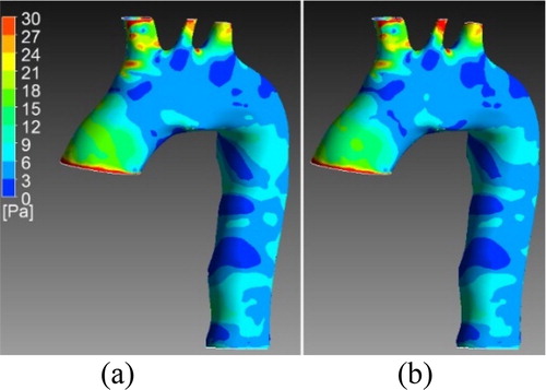
Figure 2. Pressure wall at systole for one validation case. a) Results from the simulation b) Results from the ROM.

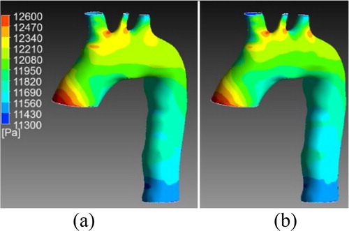
We can observe a good correspondence between the results of the two ROM in the systole part. In diastole, it is more complicated to learn correctly the output since the variable have small values. Same observations can be made for the ROM computing the velocity fields. In systole, the blood flow patterns (turbulences) are well described.

4. Conclusions

In this paper, ROMs were computed from 3 D transient fluid simulation returning 3 D results for any set of boundary conditions. While fluid simulations converged in several hours, the ROMs return the results in a few seconds. The results in systole are accurate enough to replace fluid simulation. We can observe that the areas with the highest values in simulation are well retrieved with the ROM. Since, area with the highest pressure at wall or WSS can be factor for further developpement of aneurysms or dissection, we believe our method could be used as predictive model.

Since those results can be computed for any set of boundary conditions, different scenarios can easily be modelised with results in real time, like for example a patient running or under a medication lowering it global blood pressure.

Disclosure statement

No potential conflict of interest was reported by the authors.

References

- Alimohammadi M, Sherwood JM, Karimpour M, Agu O, Balabani S, Díaz-Zuccarini V. 2015. Aortic dissection simulation models for clinical support: fluid-structure interaction vs. rigid wall models. Biomed Eng Online. 14(1):34.
- Canchi T, Kumar SD, Ng EYK, Narayanan S. 2015. A review of computational methods to predict the risk of rupture of abdominal aortic aneurysms. BioMed Res Int. 2015:1–12.
- Feher J. 2018. 3D transient reduced order modelling of vascular constriction model. Researchers' Conference “Frontiers of Simuation and Experimentation for Personalised Cardiovascular Management and Treatment”.
- Mendis S, Puska P, Norrving B, World Health Organization. 2011. Global atlas on cardiovascular disease prevention and control. Geneva: World Health Organization.
- Zhu Y, Chen R, Juan Y-H, Li H, Wang J, Yu Z, Liu H. 2018. Clinical validation and assessment of aortic hemodynamics using computational fluid dynamics simulations from computed tomography angiography. Biomed Eng Online. 17(1):53.