Influence of ankle joint model on lower limbs kinematics and kinetics during table tennis forehand drive

1

Keywords:

• Ankle model
• table tennis
• lower limbs
• musculoskeletal model

1. Introduction

Sport research is a key to improve performance and to prevent the risk of injury. In table tennis, many injuries are located at the upper limbs, but also at the hip joint (Nguyen et al. 2016). To investigate the origin of these hip injuries, both joint kinematics and kinetics should be taken into account.

To investigate sport biomechanics while limiting the detrimental effect of soft tissue artifacts on kinemtics and kinetics, musculoskeletal models have been developped. In a recent model dedicated to study running biomechanics (Raabe and Chaudhari 2016), the ankle was still modeled as a two degrees of freedom joint between the tibia and the talus and defined by two intersected and orthogonal axes located at the center of the talus: one is a medio-lateral axis (perpendicular to the longitudinal axis of the tibia) and the other is a postero-anterior axis.

However, this ankle joint definition does not appear as physiologic as a model that would incorporate a first axis defined between distal malleoli extremities (Brockett and Chapman 2016) and the Henke axis (Henke 1863).

To investigate the potential impact of this model on ankle biomechanics and its propagation to upper joints such as knee and hip joints, the purpose of this study was to assess the impact of ankle joint model on the lower limbs kinematics and kinetics during table tennis top spin forehand drive. The hypothesis was that the more physiologic ankle model could impact ankle biomechanics but also this of upper joint such as the hip.

2. Methods

2.1. Participants

Sixteen French international table tennis players (thirteen male and three female) participated in this study, which was ethically approved (2018-A00173-52). On average, subjects’ characteristics were: age 19.5 ± 4.6 y.o., mass 69.9 ± 7.0 kg, height 1.80 ± 0.05 m for male; and age 23.3 ± 3.7 y.o., mass 57.6 ± 2.5 kg, height 1.70 ± 0.01 m for female.

After receiving their written consent, participants were equipped with 91 reflective markers placed on the whole body and the racket. Motion capture acquisitions were performed with a 15-cameras optoelectronic motion capture system (Vicon® System, ©Oxford Metrics Inc., UK, 200 Hz) with simultaneous recording of ground reaction forces obtained with two force plates (AMTI OR6, USA, 1000 Hz).

Motion capture acquisitions were performed to measure markers trajectories and force plate data during top spin forehand drive in opposition with a player with a similar level. Five trials composed of five successive top spin forehand drives were recorded for each participant. A trial with at least 5 forehand strokes with the dominant foot on the platforms was selected for this study.

Right after the motion capture and without removing the markers, participants underwent a low dose biplanar radiographic acquisition (EOS, EOS Imaging) in a neutral standing posture. 3 D reconstruction of the spine, pelvis, femurs, tibias and fibulas were performed and used to personalize the biomechanical model.

2.2. Ankle model

Ankle flexion/extension axis was defined using distal parts of the tibia/fibula meshes where both malleoli region were located. The abduction/adduction axis, of the Raabe and Chaudhari (2016) model has been locked, and the Henke axis in the subtalar joint, which was already present but locked in this model, was unlocked.

2.3. Data treatment

To quantify the effect of the ankle model, a first model was built for all subjects based on the model of Raabe and Chaudhari (2016) and personalized for hip and knee joints. Then, the resulting model (M1) was duplicated and the second was modified for the ankle joint acording to the definition describe above to provide a more physiological model (M2).

Kinematic data were then processed using both models through a multibody kinematic optimization, performed in OpenSim 3.3 (Delp et al. 2007) and followed by an inverse dynamic processing performed in Matlab to obtained joint moment in a proximal orthogonal coordinate system. The root mean square difference (RMSD) and the maximum difference (Diff max) between the two models were computed for both joint angle and moments of the lower limbs joints. The root mean square error (RMSE) of the markers reconstruction with the two models was also computed and compared.

3. Results and discussion

Markers RMSE did not changed noticeably between the two methods, which means two equivalent suitable configurations were obtained with the two models that during the multibody kinematics optimization, OpenSim could find.

Maximum differences, RMSD and range of both kinematics (Table 1) and kinetics were higher, as expected, for the ankle than on the other joints. Regarding kinematics, RMSD and the maximum difference were found higher on the ankle than on any other joint. Nevertheless, the difference is not negligible on the hip and knee joints with a maximum difference reaching up to 7° on the playing side hip rotation, which corresponded to 20% of the range of motion.

Table 1. Mean kinematics results for playing side (PS) and non-playing side (NPS) for all the participants. Range: range of motion of the degree of freedom.

			RMSD (°)	Diff max (°)	Range (°)
Hip	Flexion	PS	1.4	3.0	59.8
		NPS	1.2	2.4	47.6
	Abduction	PS	1.8	3.2	27.3
		NPS	1.9	3.5	17.6
	Rotation	PS	3.4	6.8	34.5
		NPS	3.5	6.2	36.9
Knee	Flexion	PS	0.6	1.1	41.4
		NPS	0.5	1.0	33.7
Ankle	Flexion	PS	11.4	14.6	27.0
		NPS	6.7	10.1	35.9

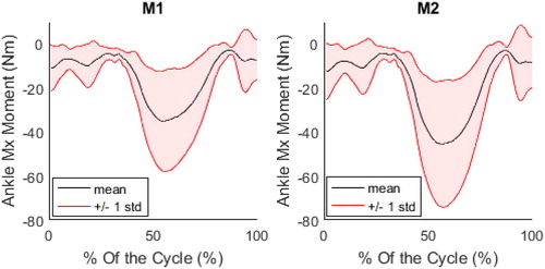
Regarding kinetics, on average for all the participants, RMSD on the playing side joint moments were 4.3, 5.3 and 7.0 Nm for hip in the 3 directions of the pelvis coordinate system (maximum differences: 11.9, 13.9 and 20.5 Nm, respectively) for range magnitudes of 500, 423 and 491 Nm. For the knee, RMSD was 4.2, 2.2 and 3.4 Nm following the 3 axis of the coordinate system (maximum differences: 10.2, 6.0 and 8.7 Nm, respectively) for range magnitudes of 184, 246 and 191 Nm. For the ankle (Figure 1), RMSD was 2.4, 0.5 and 0.6 Nm in the three direction of the coordinate system located at the center of the talus (maximum differences: 5.7, 1.5 and 0.6 Nm, respectively) for range magnitudes of 30, 28 and 98 Nm.

Figure 1. Evolution of the ankle Mx moment for one subject on both methods. M1 on the left and M2 on the right.

4. Conclusions

This study aimed at evaluating the impact of ankle personalization on lower limbs kinematics and kinetics. It has been found that there was no difference in the RMSE despite the change of model.

However, differences in kinematics and kinetics have been observed. Even if the higher difference were observed on the ankle angles and moments, the other lower limbs joints were also impacted by the model difference.

Due to the impact on biomechanical results of the ankle model, even when looking at the hip joint, the more physiological ankle description of the model incorporating the mediolateral malleoli axis and Henke axis can be recommended to investigate biomechanics of table tennis. Personnalization of the flexion/extension axis can be done based on 3 D reconstructions from EOS biplanar radiographic images. The personnalization of the Henke axis could also be done but would necessitate additional radiographic acquisitions that are unnecessary (Nichols et al. 2017).

Acknowledgements

Authors would like to thank the French federation of table tennis for their help for recruiting table tennis players, and the volunteers.

References

- Brockett CL, Chapman GJ. 2016. Biomechanics of the ankle. Orthop Trauma [Internet]. 30(3):232–238.
- Delp SL, Anderson FC, Arnold AS, Loan P, Habib A, John CT, Guendelman E, Thelen DG. 2007. OpenSim : open-source software to create and analyze dynamic simulations of movement. 54:1940–1950.
- Henke J. 1863. Handbuch der Anatomie und Mechanik der Gelenke. CF Winter’sche Verlagshandlung.
- Nguyen S, Sauret C, Bourgain M, Le Garrec S, Jacquet-Yquel R, Palierne C, Rouch P, Thoreux P. 2016. Pathologies coxo-fémorales des pongistes de haut niveau. In: SFTS-SFMES. Pau, France.
- Nichols JA, Roach KE, Fiorentino NM, Anderson AE. 2017. Subject-specific axes of rotation based on talar morphology do not improve predictions of tibiotalar and subtalar joint kinematics. Ann Biomed Eng. 45(9):2109–2121. [Internet].
- Raabe ME, Chaudhari A. 2016. An investigation of jogging biomechanics using the full-body lumbar spine model: model development and validation. J Biomech. 49(7):1238–1243. [Internet]