
1. Introduction
Numerical modelling is an effective tool to broaden our knowledge about the knee joint. As a result, many Finite Element (FE) and musculoskeletal (MSK) models of the knee with various levels of complexity have been proposed (Hume et al. 2018; Mo et al. 2018; Rajagopal et al. 2016). Muscles have a crucial role in controlling the joint kinematics and producing stability during movements. In the classical musculoskeletal (MSK) modelling technique, the muscles are modelled as 1 D structures which facilitates simulating joint kinematics but is not capable of monitoring the stress and strain distribution inside the 3 D anatomical structures. There are also some MSK modelling platforms that provide support for multipoint muscles, which are similar to axial muscles, except that they can contain multiple via points and wrap around obstacles. This allows the associated muscle force directions to vary when the muscle is wrapped around the bone during movement. However, it is clear that as long as the muscles are treated as 1 D structures, the muscle insertion area and the contacts/sliding between different muscles are not taken into account. This can be addressed by using FE modelling technique that enables us to model the soft tissues in 3 D and capture their individual contribution throughout joint movement. Nevertheless, developing a full 3 D FE model of the lower limb can be time consuming and requires a higher computational cost. Thus, depending on the objective of the simulation, the question of which modelling technique serves the best remains. Therefore, the objective of this study is to evaluate the effect of using either of the aforementioned muscle modelling techniques on the extracted tibiofemoral kinematics during knee flexionextension.
2. Methods
A biomechanical model of the lower limb of a volunteer subject has been created in ArtiSynth which is a free 3 D modelling platform supporting the combined simulation of multibody and finite element models and provides support for both multipoint 1 D and 3 D active muscles (www.artisynth.org. . . . . . . . . . ). This model includes the joint constraining ligaments, the hamstring muscle group (biceps femoris, semimembranosus and semitendinosus) and the quadriceps femoris muscle group (rectus femoris, vastus lateralis, vastus medialis and vastus intermedius). The Rectus Femoris muscle is modelled using three different techniques. In the first case, it is modelled using a 1 D muscle model defined between the muscle insertions on the patellar and femoral bones while respecting the muscle moment arm. In the second case, it is modelled as a 1 D multipoint muscle that has to pass through multiple via points defined based on the 3 D geometry of the patient’s muscle and it can wrap around the femur bone when it comes to contact with it. In the third case, the muscle is modelled as an active 3 D FE model which is in contact with the surrounding passive muscles (assumed as rigid bodies in this preliminary study). The hamstring muscle group is modeled as 1 D in all the cases. The flexion of the joint is simulated (forward dynamics) and the kinematics of the tibiofemoral joint is compared between the three different cases to evaluate the effect of these different techniques on the kinematics.
2.1. Geometry and FE mesh generation
A combination of Computerized Tomography (CT) and Magnetic Resonance Imaging (MRI) data obtained from a volunteer subject were used to acquire the desired tissue geometries. The CT scan images were acquired with 7 mm axial intervals, and 0.83 mm sagittal and coronal intervals to reconstruct the bones. The MRI images of the lower limb with 6.99 mm axial intervals and 0.97 mm sagittal and coronal intervals were used to reconstruct the muscle parts. Knee joint MRI images with 0.7 mm axial intervals and 0.31 mm sagittal and coronal intervals were used to obtain the exact position of the ligaments and tendons insertions. Manual segmentation was performed in Amira software to extract the 3 D geometries (Elyasi et al. 2019). The Rectus Femoris muscle geometry was then processed and converted to solid 8-node hexahedral elements using a sculpt meshing algorithm.
2.2. Material properties
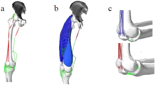
The bones were modeled as rigid bodies. All the constraining ligaments including the patellar ligament, the lateral and medial patellar retinaculum ligaments, the collateral and cruciate ligaments and the anterolateral ligament were modeled as 1 D linear spring elements having 150 N/mm stiffness (Woo et al. 1991). The hamstring muscle group was modelled as 1 D while conserving the muscles’ anatomical moment arms. The 3 D active muscles consist of an active part using the Blemker constitutive model (Blemker et al. 2005) and a passive part considered to be neo-Hookean hyperelastic (Luboz et al. 2018) Muscle fibers are distributed along the length of the muscle in the direction of the vector connecting the muscle insertion sites. The quadriceps tendon attached to the 3 D rectus Femoris muscle was modeled as multipoint springs being able to wrap around the femur bone ().
Figure 1. FE model of the thigh with (a) 1 D muscles (b) 3 D muscles (c) Top: 1 D quadriceps tendon wrapped around the Femur bone in flexed knee, Bottom: 1 D quadriceps tendon without wrapping in flexed knee.
2.3. Boundary conditions and constraints
The femur was fixed in its initial position and the tibia and patella were left unconstrained throughout the simulation. The hamstring muscle group was activated to put the knee in the flexed position. Contact has been defined between all the bones and muscle components, having frictionless tangential behavior and hard normal behavior.
3. Results and discussion
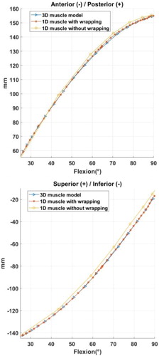
The anteroposterior and superoinferior movements of the tibia with respect to femur coordinate system (Azmy et al. 2010) are demonstrated in . The flexion range of the knee model starts at 25 degrees of flexion and continues to 90 degrees of flexion. The tibia continues to move posteriorly and superiorly as the knee undergoes flexion. The Root Mean-Square Error (RMSE) is calculated to compare the extracted kinematics of the model with 3 D Rectus Femoris muscle with the models having 1 D muscles with and without wrapping. The extracted kinematics from the model having 1 D muscles with wrapping are closer to the 3 D muscle model in both the anteroposterior and superior/inferior degrees of freedom (Ant/Post RMSE 0.6 mm vs. 2.2 mm, Sup/Inf RMSE 0.3 mm vs. 3.8 mm respectively for the model with and without wrapping). In conclusion, the results of this study suggest that using the multipoint 1 D muscles that can wrap around the bony tissues can result into closer kinematic outcomes to the 3 D muscle models.
Figure 2. Extracted knee kinematics.
Additional information
Funding
References
- Azmy C, Guérard S, Bonnet X, Gabrielli F, Skalli W. 2010. EOS orthopaedic imaging system to study patellofemoral kinematics: assessment of uncertainty. Orthop Traumatol Surg Res. 96(1):28–36.
- Blemker SS, Pinsky PM, Delp SL. 2005. A 3D model of muscle reveals the causes of nonuniform strains in the biceps brachii. J Biomech. 38(4):657–665.
- Elyasi, et al. 2019. ISB Conference Proceedings.
- Hume DR, Navacchia A, Ali AA, Shelburne KB. 2018. The interaction of muscle moment arm, knee laxity, and torque in a multi-scale musculoskeletal model of the lower limb. J Biomech. 76:173–180.
- Luboz V, Bailet M, Boichon Grivot C, Rochette M, Diot B, Bucki M, Payan Y. 2018. Personalized modeling for real-time pressure ulcer prevention in sitting posture. J Tissue Viability. 27(1):54–59.
- Mo F, Li F, Behr M, Xiao Z, Zhang G, Du X. 2018. A lower limb-pelvis finite element model with 3D active muscles. Ann Biomed Eng. 46(1):86–96.
- Rajagopal A, Dembia CL, DeMers MS, Delp DD, Hicks JL, Delp SL. 2016. Full-body musculoskeletal model for muscle-driven simulation of human gait. IEEE Trans Biomed Eng. 63(10):2068–2079.
- Woo SL-Y, Hollis JM, Adams DJ, Lyon RM, Takai S. 1991. Tensile properties of the human femur-anterior cruciate ligament-tibia complex. Am J Sports Med. 19(3) :217–225.