An open-source musculoskeletal model of the lumbar spine and lower limbs: a validation for movements of the lumbar spine

Abstract

Musculoskeletal models of the lumbar spine have been developed with varying levels of detail for a wide range of clinical applications. Providing consistency is ensured throughout the modelling approach, these models can be combined with other computational models and be used in predictive modelling studies to investigate bone health deterioration and the associated fracture risk. To provide precise physiological loading conditions for such predictive modelling studies, a new full-body musculoskeletal model including a detailed and consistent representation of the lower limbs and the lumbar spine was developed. The model was assessed against in vivo measurements from the literature for a range of spine movements representative of daily living activities. Comparison between model estimations and electromyography recordings was also made for a range of lifting tasks. This new musculoskeletal model will provide a comprehensive physiological mechanical environment for future predictive finite element modelling studies on bone structural adaptation. It is freely available on https://simtk.org/projects/llsm/.

Keywords:

• Musculoskeletal modelling
• subject-specific
• full-body
• lumbar spine
• subject-derived

1. Introduction

Musculoskeletal models are a powerful tool to investigate various musculoskeletal conditions and have a range of clinical applications when used for predictive modelling. Such models of the lumbar spine can be used to investigate lumbar pathologies such as spine deformities, osteoarthritis or intervertebral disc degeneration, and inform surgical and non-surgical treatment interventions. The accurate estimation of muscle and joint reaction forces they provide for specific tasks can even be combined with finite element models of the lumbar vertebrae to investigate bone remodelling and fracture risk. Musculoskeletal models of the lumbar spine have been developed in previous studies. However, a number of limitations are associated with these models making them unsuitable for applications requiring a high level of detail and accuracy during complex tasks. Focusing on open-source models developed in OpenSim (Delp et al. 2007), it is common for model developers to build upon and combine existing models. Christophy et al. (2012) developed a musculoskeletal model of the lumbar spine incorporating an extensive lumbar musculature. This model was later enhanced by Senteler et al. (2016) through the use of bushing elements at lumbar levels to model intervertebral stiffness. Although these models are substantially detailed, the muscle architecture is based on different cadaveric datasets which may not be consistent with each other. Bruno et al. (2015) proposed a new method to adjust muscle moment arms and cross section areas based on medical imaging to overcome this limitation. However, these models are all restricted to the spine and have to be combined with other models of the lower limbs to allow appropriate full-body studies of daily living activities (McGregor and Hukins 2009). In response to this need, full-body models have been developed more recently. Raabe and Chaudhari (2016) combined the lumbar spine model from Christophy et al. (2012) with the lower limb models from Hamner et al. (2010) and Arnold et al. (2010) to investigate jogging biomechanics. In a similar manner, Actis et al. (2018) combined the lumbar spine model from Christophy et al. (2012) with the lower limb model from Delp et al. (1990), and validated their model for flexion, extension, lateral bending and axial rotation of the spine separately. These types of activities do not involve large movements of the spine and further validation is necessary for a study of the back where lifting tasks are examined. Beaucage-Gauvreau et al. (2019) increased the spine range of motion and muscle tetanic stress of the Raabe and Chaudhari (2016) model, and validated this new model for lifting tasks. However, these combined models are based on generic bone geometries obtained from different datasets, which potentially results in inconsistent joint locations and unrealistic muscle paths. This is particularly true when combining spine and lower limb models. Modelling the spine-pelvis-hip complex accurately is of particular importance when studying locomotion activities and balance strategies. Yet, the position of the hip joint relative to the position of L5-S1 joint and the location of muscle insertions in that region necessarily depend on the shape of the pelvis. Other spine-focused musculoskeletal models have also been developed following a similar approach, especially on the proprietary platform provided by AnyBody Technology (de Zee et al. 2007; Han et al. 2012; Ignasiak et al. 2016; Bassani et al. 2017).

The current study proposes a new full-body musculoskeletal model including the head and upper limbs, with a detailed representation of the lower limbs and the lumbar spine. Bone geometry, muscle paths and muscle insertions were all obtained from full-body magnetic resonance images (MRI) of a single young healthy subject to ensure the consistency of the anatomy throughout the model. Assessment of the model was carried out over a large range of motion to ensure simulation of lifting tasks and balance recovery will be possible in future research. Segmentation of the anatomical geometry also guarantees this model will be compatible with predictive finite element modelling approaches to investigate bone structural adaptation under physiological loading conditions.

2. Methods

2.1. Data acquisition

To ensure consistency within the model and during the simulations, a protocol was developed to acquire from a subject the detailed anatomical description necessary to build a full-body musculoskeletal model, along with movement data and ground reaction forces needed for musculoskeletal simulations. For this study, a healthy young male volunteer (26 years, 175 cm, 67.8 kg) with no history of back pain or other condition of the spine and lower limbs was recruited. The study was granted ethical approval by the NHS Health Research Authority (REC reference: 17/HRA/0465) and the Imperial College Research Ethics Committee (ICREC reference: 17IC3811), and the volunteer gave written informed consent.

2.1.1. Everyday life activities

The volunteer was asked to perform activities representative of daily living in the safe environment of the Human Biodynamics Lab in the Imperial College Research Labs at Charing Cross Hospital (London, UK). These activities include walking, standing up and sitting down, going up and down stairs, as well as the following spine specific movements: forward flexion and maximal flexion with finger tips to toes, extension, lateral bending on both sides, axial rotation on both sides, sitting upright and sitting flexed forward, and lifting a 5 kg box from the ground at different angles and in sitting and standing positions. Kinematic data were recorded using a 10-camera passive optical motion capture system (Vicon T160, sampling rate 100 Hz, Oxford Metric, Oxford, UK) with a comprehensive marker set of 77 markers (Table A1, supplementary material). Muscle activations were also recorded using wireless surface electromyography (sEMG) (Myon320, sampling rate 1000 Hz, Myon AG, Schwarzenberg, Switzerland). Pairs of self-adhesive gel-coated electrodes (Neuroline 720 00-S/25, Ambu A/S, Ballerup, Denmark) were placed bilaterally on the longissimus and iliocostalis following the SENIAM project (Surface Electromyography for the Non-Invasive Assessment of Muscles) guidelines (Hermens et al. 1999).

Table 1. Kinematic constraint coefficients from Rozumalski et al. (2008).

	Flexion-extension	Lateral bending	Axial rotation
L1–L2	0.179705	0.187939	0.213982
L2–L3	0.208948	0.250128	0.209729
L3–L4	0.221445	0.245332	0.183679
L4–L5	0.210822	0.181086	0.200691
L5–S1	0.179080	0.135515	0.191919

Ground reaction forces and moments were measured with three forceplates (Type 9286BA, sampling rate 1000 Hz, Kistler Instruments Ltd., Hook, UK) which could be moved into different configurations depending on the activity. All experimental data were collected with Nexus (Oxford Metric, Oxford, UK) and processed with Nexus, MATLAB (The MathWorks, Inc.) and the Biomechanical ToolKit (Barre and Armand 2014).

2.1.2. MRI scan protocol and image processing

An imaging protocol was developed at the Charing Cross Hospital imaging facility (London, UK) to acquire radiation-free full-body axial anatomical images in the supine position using a 3T Siemens Verio MRI scanner (Siemens AG, Erlangen, Germany). A 3D T1-weighted VIBE (volumetric interpolated breath-hold examination) sequence was used to acquire high resolution images of the spine region from C7 to the mid femur. The signal was received through a spine coil and two body matrix coils, with MRI protocol settings as follow: axial field of view 450 × 365.625 mm with a pixel size of 1.40625 × 1.40625 mm, slice thickness 1 mm, slice gap 1 mm. A 2D T1-weighted TSE (Turbo Spin Echo) sequence was used to acquire low resolution images of the head, neck and lower limbs. The signal was received through a head and neck coil, two body matrix coils and a spine coil, with MRI protocol settings as follow: axial field of view 470 × 470 mm with a pixel size of 1.46875 × 1.46875 mm, slice thickness 6 mm, slice gap 9.6 mm. Images were acquired in axial blocks of 224 and 22 slices for the high and low resolution acquisitions, respectively, with an overlap of 50 mm between adjacent blocks. The full-body scan consisted of four high resolution sections and eight low resolution sections. The total acquisition time for the full body was approximately 45 min. The high resolution sequence was selected to highlight bone, muscles, fat and other soft tissues of the spine and pelvis at the same time, while the low resolution sequence was sufficient to distinguish muscle contours and bone geometry of the lower limbs.

Bones and muscles of the spine and lower limbs were manually segmented in Mimics (Mimics Research 19.0, Materialise NV, Leuven, Belgium) by the first author. The 3D geometry was obtained from the 2D segmented slices using the Mimics 3D reconstruction, wrapping and smoothing tools. Visual verification of the accuracy of the obtained geometries was carried out by superimposing 3D contours on 2D images.

Cod liver oil capsules of 500 mg were placed in the same location as the reflective motion capture markers during MRI scanning. Marker positions were then found from MRI scans and adjusted in the OpenSim model to ensure an exact match between virtual and experimental markers.

2.2. Building the musculoskeletal model

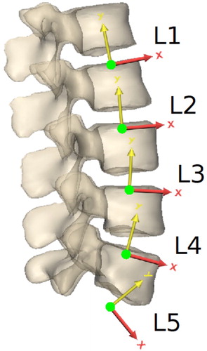
A full-body musculoskeletal model (Figure 1) based on the healthy young male volunteer was implemented in OpenSim 3.3 (Delp et al. 2007). It is bilateral and composed of 20 rigid bodies articulated with 19 joints for a total of 45 degrees of freedom (Figure A1, supplementary material): hips (three rotations each), knees (one rotation each), patello-femoral joints (one rotation each) and ankles (two rotations each) for the lower limbs, shoulders (three rotations each) and elbows (two rotations each) for the upper limbs, five lumbar joints (three rotations each), T7–T8 joint (three rotations) and C7–T1 joint (three rotations) for the spine. Each of the five lumbar joint centres is located at the intersection of the flexion-extension instantaneous axis of rotation as defined by Pearcy and Bogduk (1988) with the mid-sagittal plane (Figure 2). The flexion-extension axis is pointing dextro-laterally. The axis of rotation for lateral bending is orthogonal to the flexion-extension axis of rotation, parallel to the vertebra’s proximal endplate plane as defined by Pearcy and Bogduk (1988) and pointing anteriorly. The axial rotation axis is orthogonal to the flexion-extension and lateral bending axes, pointing cranially. In the three-segment thoracic and cervical spine, T7–T8 and C7–T1 joints are also ball and socket joints, with the joint centre being at the centre of the intervertebral disc. Lower and upper limbs joint definitions are based on the definitions given in existing models (Modenese et al. 2011; Rajagopal et al. 2016) and adjusted to fit the subject’s geometry obtained with MRI.

Figure 1. Musculoskeletal model of the lower limbs and lumbar spine with 538 musculotendon actuators.

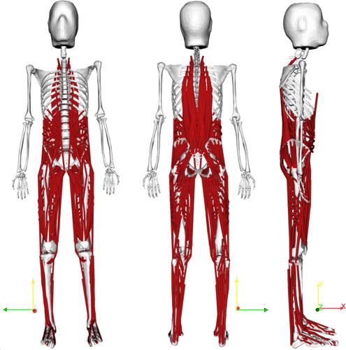
Figure 2. Location and orientation of the local lumbar vertebral coordinate systems, as defined by Pearcy and Bogduk (1988).

For each body segment, mass, centre of mass and matrix of inertia were derived from the MRI scans by assigning an initial density of 1.92 g.cm⁻³ to all bones and 1.05 g.cm⁻³ to all soft tissues (International Commission on Radiological Protection 2009). The bone density value was gradually adjusted to 1.50 g.cm⁻³ for a perfect match between the total body mass obtained with this method and the actual weight of the subject.

The model includes 538 musculotendon actuators to represent 92 muscles of the lower limbs and lumbar spine. Muscle actuators were adapted from existing musculoskeletal models (Modenese et al. 2011; Christophy et al. 2012; Bruno et al. 2015) and implemented with the Thelen musculotendon model (Thelen 2003) available in OpenSim. Muscle geometries were adapted to the subject-derived bone geometries by defining muscle insertions, attachments and path points from the MRI scans of the healthy volunteer. Tendon slack lengths and optimal fibre lengths from the generic models were scaled with the OpenSim scaling tool to match the anatomy of the volunteer. Maximum isometric forces of muscles of the lumbar spine and lower limbs were increased by changing the maximum muscle tetanic stress to 100 N.cm⁻² (Bruno et al. 2015; Beaucage-Gauvreau et al. 2019). These forces are therefore not specific to the volunteer, but are more appropriate to match the physical capacities of a young active subject and allow future simulations of more complex activities including lifting tasks. Reserve actuators are used at T7–T8 to account for the back muscles that are not modelled at the ribcage level. Since the head and upper limbs are included for inertia effects only, muscles spanning the C7–T1, shoulder and elbow joints are not included and coordinate actuators providing pure moments are used at the joints.

Intervertebral joint stiffness was implemented in the model with linear bushing elements adapted from a model developed by Senteler et al. (2016) and located between each lumbar vertebra. They apply reaction moments in response to rotations between the segments they are attached to. The bushings were positioned so that no reaction moment was produced in the supine position, considered as a neutral position. Bushing stiffness values for each lumbar level and each degree of freedom are shown in Table A2 (supplementary material).

Table 2. Comparison between muscle activation predicted with the model and measured with sEMG on the right and left longissimus and iliocostalis of the same subject for the three activities shown in Figure 12.

Activity	Assessment method		Right longissimus	Right iliocostalis	Left longissimus	Left iliocostalis
(A) Forward flexion from standing	(1)	Magnitude error Phase error Combined error	15.7% 7.8% 17.6%	16.8% 10.8% 20.0%	8.3% 12.0% 14.7%	5.0% 12.5% 13.4%
	(2)	Agreement	96.8%	89.1%	70.5%	82.0%
	(3)	xcorr-value	0.970	0.943	0.929	0.924
(B) Forward flexion from sitting	(1)	Magnitude error Phase error Combined error	–3.9% 9.4% 10.2%	–4.5% 5.6% 7.2%	19.4% 7.9% 21.0%	–0.6% 10.2% 10.2%
	(2)	Agreement	77.2%	82.5%	78.9%	93.0%
	(3)	xcorr-value	0.957	0.984	0.969	0.949
(C) Lifting 5 kg from the ground	(1)	Magnitude error Phase error Combined error	0.2% 10.7% 10.7%	–0.8% 12.4% 12.4%	14.3% 6.9% 15.8%	–10.7% 9.9% 14.6%
	(2)	Agreement	82.3%	80.7%	90.3%	69.4%
	(3)	xcorr-value	0.944	0.925	0.977	0.952

Three comparison methods are used. The method from Lund et al. (2011), (1) measures dissimilarity between the two signals using a magnitude error, a phase error and a combined error coefficient. The method proposed by Actis et al. (2018), (2) quantifies the agreement between model activations and sEMG measurements as the percentage of the trial where both signals are either above or below a 50% activation threshold at the same time. The method used by Beaucage‐Gauvreau et al. (2019), (3) is based on cross‐correlation values (xcorr‐values) for a time lag of zero between the two signals.

Skin artifacts are particularly large in the back making tracking the movement of individual vertebrae difficult with standard motion capture where markers are taped directly on the skin. White et al. (1978) demonstrated that individual lumbar vertebrae can be assumed to move as a linear function of the overall movement of the spine, which can be tracked more accurately. Based on this assumption, it is common practice to use linear kinematic constraints at each lumbar level for all degrees of freedom (Christophy et al. 2012; Han et al. 2012; Ignasiak et al. 2016; Raabe and Chaudhari 2016; Bassani et al. 2017; Actis et al. 2018; Beaucage-Gauvreau et al. 2019). Coefficients for these kinematic constraints are usually derived from in vivo experiments (Dvorak et al. 1991; Arjmand and Shirazi-Adl 2006; Wong et al. 2006; Fujii et al. 2007; Rozumalski et al. 2008) where individual lumbar rotations are expressed as a function of an overall spine angle. However, this overall angle is measured between the pelvis and either L1, T12, T1 or the shoulders, depending on the study. It is therefore crucial to ensure the musculoskeletal modelling approach is compatible with the experimental methods used to measure coupling coefficients by choosing an adequate thoracic spine representation and tracking it accurately. Such considerations are sometimes neglected in existing models, potentially resulting in an erroneous estimation of the lumbar kinematics, especially for large movements of the spine. In the current model, kinematic constraint coefficients for flexion extension, lateral bending and axial rotation are taken from the study by Rozumalski et al. (2008) which expresses each lumbar intervertebral angle as a function of the angles between L1 and S1 (Table 1). The modelling choices made for the spine are consistent with this data set. The three-segment thoracic and cervical spine makes it possible to track separately the lower thoracic spine, upper thoracic spine, and head which ensures anatomically correct lumbar spine movements and accurate positioning of the shoulders and head for large spine movements. Greater consistency between rotations in the three anatomical planes is also ensured as all coefficients come from the same data set.

The experimental markerset of 77 markers was implemented on the model for inverse kinematics simulations (Figures A2 and A3, supplementary material). The numerous markers used on the spine allow spinal regions to be tracked despite skin artifacts. By equally weighting the virtual markers of a single rigid body during inverse kinematics, OpenSim will average the position of this segment to match all the experimental markers attached to it with the same accuracy.

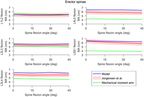
Figure 3. Model moment arms (in blue) at the lumbar joints for the erector spinae compared to experimental data (in red) reported by Jorgensen et al. (2003). The shaded area is one standard deviation. The moment arms calculated with the mechanical approach are shown in green. Right and left side moment arms from the model were very similar so only the right side is shown here.

2.3. Assessing the musculoskeletal model

Muscle geometry was derived from MRI scans of the healthy subject lying in a supine position. Muscle moment arms were checked for the range of motion the model is intended to be used for by ensuring they are physiologically feasible, with no discontinuity. Although the lower limbs of this full-body model are adapted from a model that has been extensively assessed at the hip (Modenese et al. 2011; Modenese and Phillips 2012; Modenese et al. 2013), muscle moment arms were compared against literature values at the hip, knee and ankle joints (Grood et al. 1984; Németh and Ohlsén 1985; Dostal et al. 1986; Spoor and van Leeuwen 1992; Buford et al. 1997; Delp et al. 1999; Arnold et al. 2000; Maganaris 2004; Blemker and Delp 2005; Fath et al. 2010). Erector spinae moment arms were compared with values from Jorgensen et al. (2003). In accordance with Jorgensen et al. (2003), moment arms were calculated at each lumbar level as the distance between the centroid of the erector spinae and the centroid of the intervertebral disc in a plane through and parallel to the disc. For reference, erector spinae moment arms were also calculated with the mechanical approach, where the moment arm is the shortest distance between the joint centre of rotation and the musculotendon actuator. The difference between these two moment arm definitions is shown in Figure A4 (supplementary material). For these comparisons, the moment arm of a single muscle is the average of the musculotendon actuators’ moment arms representing this muscle. Maximum isometric moments in the lumbar spine region were also checked to ensure they are within an acceptable range.

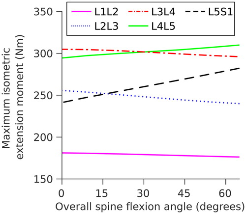
Figure 4. Maximum isometric extension moments at each lumbar level as a function of overall spine flexion.

A musculoskeletal simulation pipeline was used to estimate muscle and joint reaction forces from the experimental data. Inverse kinematics was performed to calculate joint angles. After this step, coordinate coupling constraints in the lumbar spine were removed to avoid over-constraining the model and underestimating muscle forces. Inverse dynamics was used to compute joint moments. A static optimisation problem where the sum of muscle activations squared is minimised was solved to predict muscle forces. A joint reaction analysis was also carried out to estimate joint contact forces.

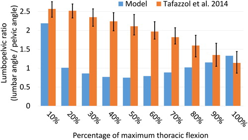
Pelvic, lumbar and thoracic angles in the sagittal plane obtained from inverse kinematics were compared to measurements from the literature for forward flexion (Tafazzol et al. 2014). In accordance with Tafazzol et al. (2014), the pelvic and thoracic angles (measured at S1 and T5 respectively) are expressed in the global coordinate system while the lumbar angle (measured at L1) is expressed in the pelvis coordinate system, all with respect to the upright standing position. The lumbopelvic ratio was calculated by dividing the lumbar angle by the pelvic angle and compared to measurements from Tafazzol et al. (2014) for intervals of 10% of full spine flexion.

Joint reaction forces estimated with the model were compared to measurements from the literature at different lumbar levels. At L4-L5 and L3-L4 levels, the comparison was made with disc pressure measured in-vivo in healthy volunteers (Nachemson 1965; Schultz et al. 1982; Sato et al. 1999; Wilke et al. 1999, 2001; Takahashi et al. 2006). At L1-L2 level, the comparison was made with forces in a vertebral body replacement (VBR) telemeterised implant (Rohlmann et al. 2008). Absolute comparison was not possible since in-vivo data is from different subjects. Data was therefore normalised to the corresponding values in the upright standing position, allowing relative comparison at all lumbar levels.

Results from musculoskeletal simulations were also assessed by comparing estimated muscle activations against sEMG signals recorded on the lumbar muscles of the same subject during the same trials. This comparison was done for basic movements of the spine at normal speed: forward flexion from standing upright, forward flexion from sitting upright and lifting a 5 kg box from the floor to the chest while standing. Using the same method applied for virtual marker placement, cod liver oil capsules of 1000 mg were used during MRI scanning to locate sEMG electrodes in the model. For each electrode, musculotendon actuators located directly below the electrode area were selected, and the average of their activations used for the comparison. Raw sEMG signals were demeaned, high-pass filtered at 30 Hz with a zero-phase fourth order Butterworth filter and rectified. Rectified signals were low-pass filtered at 10 Hz (Arnold et al. 2013; Klemt et al. 2019). Both model activations and sEMG signals were normalised to the peak filtered value for each trial. Three different metrics were used to assess the similarity between the predicted muscle activations and the measured sEMG. Lund et al. (2011) proposed a validation metric originally developed by Geers (1984) to compare waveforms between model activations and in-vivo sEMG measurements. This metric combines the magnitude error M and the phase error P between the two curves into a combined error C. M, P and C are designed to return zero when the two curves are identical. Actis et al. (2018) defined the agreement between the model predictions and the sEMG measurements as the percentage of the trial where both normalised signals are either below or above a 50% threshold at the same time. This method is less robust as a 100% agreement can be obtained even when the two curves are not matching. It was included to allow comparison with previous studies. Beaucage-Gauvreau et al. (2019) performed a cross-correlation analysis between model predictions and sEMG measurements using the MATLAB xcorr function. In this study, cross-correlation values obtained with this method are shown for a time lag of zero.

3. Results

3.1. Model verification and validation

In the lumbar spine, the erector spinae moment arms during forward flexion of the spine calculated with the method proposed by Jorgensen et al. (2003) compare well with the measurements from their study at all lumbar levels (Figure 3). Muscle moment arms of the lower limbs calculated with the mechanical definition show overall agreement with moment arms reported in the literature (Figures A5, A6, A7 and A8, supplementary material).

Maximum isometric moments at all lumbar spine levels vary between 175 Nm and 310 Nm (Figure 4) for an overall trunk flexion of 0° to 60°, and are within the range reported by Hansen et al. (2006) (171–480 Nm).

3.2. Spine angles

The spine angles obtained with the model at maximum spine flexion are within the range reported by Tafazzol et al. (2014) (Figure 5), with pelvic and lumbar rotations of 53.4° and 70.9° respectively in flexion. However, the lumbopelvic ratio varies differently across the different intervals of spine flexion (Figure 6), potentially due to a different movement strategy selected by the subject.

Figure 5. Comparison with measurements reported by Tafazzol et al. (2014) for flexion angles with respect to the upright standing position for the thorax (T5), pelvis (S1) and lumbar spine (L1). Thorax and pelvis rotations are expressed in the global coordinate system while the lumbar rotation is expressed relative to the pelvis rotation. Error bars are the range reported by Tafazzol et al. (2014).

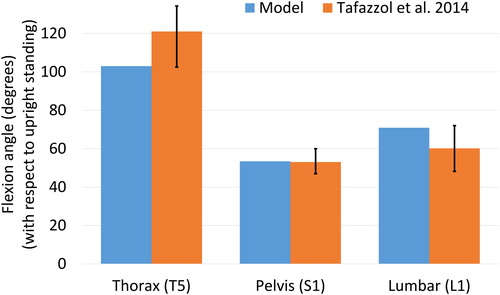
Figure 6. Comparison of the lumbopelvic ratio (lumbar angle/pelvic angle) with measurements reported by Tafazzol et al. (2014) for 10% intervals of the full spine flexion. Error bars are the range reported by Tafazzol et al. (2014).

3.3. Joint reaction forces

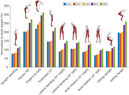
Joint reaction forces were estimated at all lumbar levels for upright standing, forward flexion at 10°, 20°, 24°, 30°, and maximal flexion with finger tips to toes, extension at 15°, lateral bending on both sides at 20°, axial rotation on both sides at 15°, sitting upright and sitting flexed forward. The subject moved in a quasi-static manner, holding each position for one second. The increment corresponding to the studied position was then selected for simulations.

Figure 7 shows the total joint reaction force at each lumbar level for these static positions. As expected, the total reaction force is higher in the lower lumbar levels. The joint reaction forces estimated with the model for each position follow the same trend for all lumbar levels. Compared to upright standing, the joint reaction force increases substantially for flexed and extended positions, while it increases to a lesser extent for lateral bending positions. Axial rotation positions have a limited influence on the joint reaction force compared to upright standing. Upright sitting slightly increases the joint reaction force compared to upright standing, potentially due to a different pelvic tilt angle when seating.

Figure 7. Total joint reaction force normalised to body weight at each lumbar level for static positions of the spine.

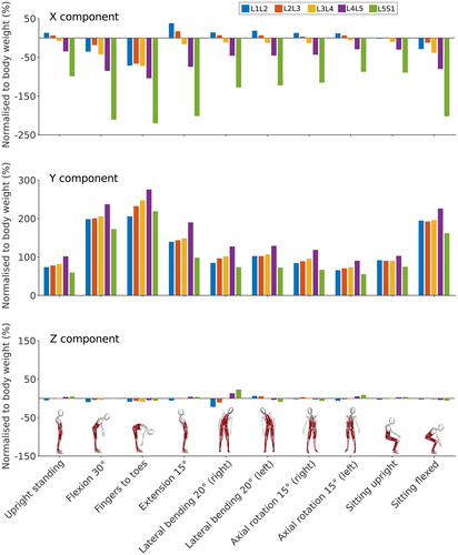
Figure 8 shows the decomposition of the total reaction force on the X, Y and Z axes of the vertebra coordinate systems. The Y component of the reaction force shows a trend similar to the total reaction force for most positions at all lumbar levels except L5-S1. At this level, the contribution of the X component is significant for all positions due to the orientation of the L5 coordinate system (Figure 2). For positions involving small movements of the spine in the sagittal plane, the X component of the reaction force is positive at the L1-L2 and L2-L3 levels and negative for the three other lumbar levels. This is due to the orientation of the vertebrae following the lumbar curvature in an upright position. For larger movements in the sagittal plane, especially spine flexion, the orientation of the vertebrae changes, and the X component of the reaction force changes sign at L1-L2 and L2-L3 levels. The contribution of the Z component in sagittally symmetric positions is minimal but not zero. For lateral bending positions, the Z component of the reaction force is higher on the right than on the left side. This potentially indicates a minor asymmetry in the subject’s spine, or is possibly a reflection of their hand dominance.

Figure 8. X (antero-posterior), Y (longitudinal) and Z (medio-lateral) components of the joint reaction force normalised to body weight at each lumbar level for static positions of the spine. Forces are expressed in the local vertebral coordinate systems shown in Figure 2.

3.3.1. L4-L5 level

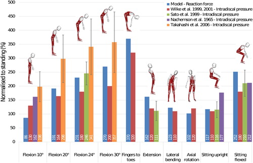
Dreischarf et al. (2013) showed that intradiscal pressure and lumbar compressive force follow a linear relationship. With this assumption, intervertebral joint reaction forces estimated with the model at L4-L5 level were normalised to upright standing and compared to in-vivo disc pressures reported in the literature (Nachemson 1965; Sato et al. 1999; Wilke et al. 1999, 2001; Takahashi et al. 2006) also normalised to upright standing (Figure 9). The model shows reasonable agreement with the pressures reported by Sato et al. (1999) and Wilke et al. (1999, 2001), with average differences of 18.2% and 23.6% respectively across all the positions considered here. The average difference with values reported by Takahashi et al. (2006) for the four poses with the spine flexed forward is higher (37.2%).

Figure 9. Comparison between in vivo intradiscal pressure (Nachemson 1965; Wilke et al. 1999, 2001; Sato et al. 1999; Takahashi et al. 2006) and joint reaction forces in the model at L4-L5 level. Error bars are one standard deviation for studies with more than one subject.

3.3.2. L3-L4 level

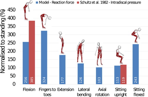
Based on the same assumption used for the L4-L5 level comparison (Dreischarf et al. 2013), the joint reaction forces estimated with the model were compared to in-vivo disc pressures reported by Schultz et al. (1982) at L3-L4 level (Figure 10). The model underestimates the normalised joint reaction force by 33% for forward flexion at 30° and by 5% for the sitting upright position. Other spine positions were not investigated by Schultz et al. (1982), however, reaction force estimations from the model are still reported here for reference.

Figure 10. Comparison between in vivo intradiscal pressure measured by Schultz et al. (1982) and joint reaction forces in the model at L3-L4 level.

3.3.3. L1-L2 level

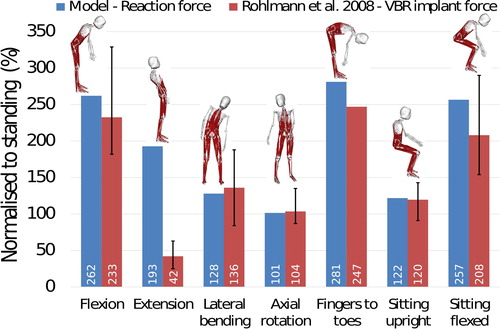
At L1-L2 level, reaction forces estimated with the model are compared against forces measured with a telemeterised VBR implant (Rohlmann et al. 2008) (Figure 11). Model estimations are within 6% of the reported values for lateral bending, axial rotation and sitting upright poses. For positions involving forward flexion of the spine, the difference between the model estimates and the measured forces is below 23%. For spine extension, the force obtained with the model is overestimated by 359% compared to the measured force.

Figure 11. Comparison between in-vivo measured forces using the VBR implant (Rohlmann et al. 2008) and joint reaction forces in the model at L1-L2 level. Errors bars represent the range.

3.4. Muscle activations

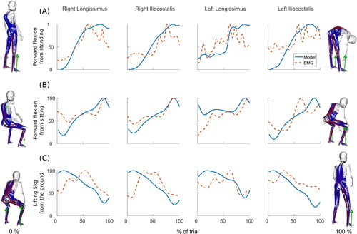
Model activations and sEMG measurements follow the same trends for the erector spinae muscles in movements involving the lumbar spine (Figure 12). Table 2 shows the agreement between the two curves calculated with three different methods. The method proposed by Lund et al. (2011) produces a combined error coefficient C which represents the dissimilarity between the two curves based on the magnitude error M and the phase error P. Negative or positive magnitude errors indicate that over the activity the predicted normalised muscle activation is lower or higher than the normalised measured sEMG, respectively. For the three activities and the four muscles considered in this study, this coefficient C varies between 7.2% (right iliocostalis in the forward flexion from a sitting position task) and 21.0% (left longissimus in the forward flexion from a sitting position task). This means that the similarity between sEMG measurements and model predictions is considered to be above 79.0%. The method proposed by Actis et al. (2018) quantifies the percentage of the activity where the two curves are in agreement. With this method, the highest agreement value is found for the right longissimus in the forward flexion from a standing position task, with model activations and sEMG measurements being in agreement during 96.8% of the trial. The lowest agreement value is found for the left iliocostalis when lifting 5 kg from the ground to a standing position (agreement during 69.4% of the trial). Using the same method as Beaucage-Gauvreau et al. (2019), there is a strong correlation between sEMG measurements and muscle activations with cross-correlation values above 0.9 for all four muscles in all three trials for a time lag of zero.

Figure 12. Model activations and sEMG activations for the right and left longissimus and iliocostalis during (A) a forward flexion of the spine from a standing upright position, (B) a forward flexion of the spine from a sitting upright position and (C) for lifting a 5 kg box from the ground to a standing upright position. Activations are normalised to the maximum activation over the activity. The stances at the beginning and end of each task are shown on the left and right of the graphs respectively.

4. Discussion

The aim of this study was to create a full-body musculoskeletal model from MRI scans of a healthy volunteer to ensure geometric consistency throughout the model. The model was developed with a detailed and physiologically feasible muscle anatomy so that it can later be combined with finite element models of the lumbar spine to investigate the potential influence of the mechanical environment on bone architecture in vertebrae. The assessment of the model is satisfactory for the intended application.

4.1. Spine angles comparison

The pelvic, lumbar and thoracic maximum flexion angles compared favourably with the measurements reported by Tafazzol et al. (2014). Differences are to be expected due to skin artifacts and marker placement. Tafazzol et al. (2014) used single inertial measurement units on the spinous process of S1, L1 and T5, which gives a precise measurement in upright standing but is subject to large skin artifacts at maximum range of motion. In the model, skin artifacts are limited by the use of marker clusters at different thoracic levels. However, as the thorax is modelled as two rigid bodies, the exact position of L1 and T5 is also approximated.

The lumbopelvic ratios obtained with the model differ largely from the ratios reported by Tafazzol et al. (2014). While this could simply be an intrinsic preference of the subject in this study, it is also worth noting that the speed of execution also differs largely between the two studies. In the study by Tafazzol et al. (2014), participants reached full flexion in 5.2 s on average, while the subject in the present study only took 2.2 s. It appears that different movement strategies can be selected depending on the speed of execution, and future research should focus on investigating these strategies across subjects and speeds.

4.2. Comparison with intradiscal pressure and joint forces

Overall, the intervertebral joint reaction forces estimated with the model are in reasonable agreement with in vivo measurements from the literature at all the investigated lumbar levels.

At L3-L4 level, there is limited agreement with the pressure measurement reported by Schultz et al. (1982) in forward flexion of the spine. In the current study, the subject performed a natural forward flexion of the spine, involving both the lumbar spine and the hips. The 30° of flexion was measured between T12 and S1. In the study by Schultz et al. (1982), the subject performed a forward flexion of 30° at the hips with a straight back and arms slightly stretched out. The difference between these two postures potentially causes the discrepancy in the lumbar loads comparison. With only two spine positions used in this comparison, the model cannot be considered validated at L3-L4 level. Joint reaction forces estimated at L3-L4 joint should therefore be used with caution if using the model in other studies.

At L1-L2 level there is limited agreement with the telemeterised VBR implant (Rohlmann et al. 2008) for the spine in extension. The forces measured by the implant are much smaller than the forces estimated by the model for this position. This is potentially due to the centre of rotation of the above vertebrae being shifted posteriorly by the implant (Rohlmann et al. 2008), reducing the load on the vertebral body for this type of movement.

In this study, comparison of intervertebral reaction forces with in-vivo intradiscal pressures was made based on the assumption of a linear relationship between reaction force and pressure in the nucleus. While this assumption is supported by previous work from Dreischarf et al. (2013), other studies have showed that disc pressure may be a non-linear function of both the compression force and the segmental angle for movements in the sagittal plane (Ghezelbash et al. 2016). Bassani et al. (2017) assessed their model at L4-L5 level using both a linear and the non-linear approach described by Ghezelbash et al. (2016), and found no significant differences between them when comparing their results to in vivo disc pressure reported by Wilke et al. (2001). As the current model will later be combined with a finite element approach and simulate a wide range of daily life activities, future work should investigate if the linear and non-linear methods for estimating disc pressure give divergent results at more extreme ranges of spine movement.

4.3. Comparison with recorded sEMG

For activities involving large movements of the spine, model activations and sEMG measurements show acceptable agreement over the trials. Activations predicted by the model follow the trends recorded with sEMG. The main discrepancies are when model activations drop close to 0% while sEMG measurements never do. This happens for upright spine positions where the model is the most kinematically stable. In these positions, joint moments calculated with inverse dynamics are close to zero and almost no muscle force is needed to balance the model. In real life, maintaining stability in an upright position requires constant postural adjustment. These small adjustments are controlled by the central nervous system which uses muscle synergies to co-activate antagonistic muscles. Muscle synergies could be deduced from inverse dynamics (Gopalakrishnan et al. 2014), and future model developments will aim at implementing these methods in the simulation pipeline. These limitations associated with static optimisation methods could also be avoided using sEMG measurements in EMG-driven simulations to account for muscle synergies (Pizzolato et al. 2015). At the current state of development, the model should therefore be more suited to accurately predict muscle activations during large and continuous movements.

4.4. Limitations and applications of the study

Although the present study is limited to one subject, it has shown that in-silico predictions of muscle activations and joint reaction forces for this particular subject agree, respectively, with the sEMG recorded on the same subject and with the range of joint reaction forces reported in the literature. Assessment of the model is satisfactory for the tasks presented here. MRI, movement data and associated ground reaction forces are being collected on other volunteers. Replicating this study for other subjects will give more confidence in the modelling approach. More complex activities combining flexion and twisting of the spine during lifting tasks will also be investigated to extend the range of use of the model. Another potential improvement would be to model ligaments in the lumbar spine instead of simulating their behaviour with the linear bushing elements. However the MRI sequences and resolution used do not provide a reliable image for segmenting lumbar ligaments, and these would have to be adapted from generic models.

Despite the limitations, the model can already be used as a generic model in a variety of research areas if scaled and with appropriate checks made beforehand (Hicks et al. 2015). As opposed to other musculoskeletal models, an advantage of this model based on a single young healthy volunteer is the consistency of both the bone geometry and the muscle anatomy across the whole body. This will enable the investigation of lumbar spine pathologies related to the lower limbs and postural alignment. The modelling technique cannot be used immediately in a clinical environment as it took a day to collect all the data from the participant and around a month to build the model from the MRI scansand to run the simulations. However, the high level of detail of this subject-derived musculoskeletal model makes it valuable for use in finite element studies which require physiological loading and boundary conditions. The developed musculoskeletal model will be combined with a structural finite element model in a bone remodelling framework previously used on the lower limbs and pelvis (Phillips et al. 2015; Zaharie and Phillips 2018). This approach will be used to predict the role of the mechanical environment in influencing lumbar vertebra structural architecture and possible damage to the structures of the spine under altered loading conditions such as asymmetric lifting of heavy loads or altered movement and control strategies, prior to the development of spinal pathologies.

Acknowledgment

The authors want to thank consultant radiologist Dimitri Amiras for reviewing the MRI scans for incidental findings.

Disclosure statement

No potential conflict of interest was reported by the authors.

Additional information

Funding

This work was supported by the Department of Civil and Environmental Engineering of Imperial College London.

References

- Actis JA, Honegger JD, Gates DH, Petrella AJ, Nolasco LA, Silverman AK. 2018. Validation of lumbar spine loading from a musculoskeletal model including the lower limbs and lumbar spine. J Biomech. 68:107–114.
- International Commission on Radiological Protection. 2009. Adult Reference Computational Phantoms. ICRP Publication 110. Ann ICRP 39(2):47–51. https://www.icrp.org/publication.asp?id=ICRP%20Publication%20110
- Arjmand N, Shirazi-Adl A. 2006. Model and in vivo studies on human trunk load partitioning and stability in isometric forward flexions. J Biomech. 39(3):510–521.
- Arnold AS, Salinas S, Hakawa DJ, Delp SL. 2000. Accuracy of muscle moment arms estimated from MRI-based musculoskeletal models of the lower extremity. Comput. Aided Surg. 5(2):108–119.
- Arnold EM, Hamner SR, Seth A, Millard M, Delp SL. 2013. How muscle fiber lengths and velocities affect muscle force generation as humans walk and run at different speeds. J Exp Biol. 216(11):2150–2160.
- Arnold EM, Ward SR, Lieber RL, Delp SL. 2010. A model of the lower limb for analysis of human movement. Ann Biomed Eng. 38(2):269–279.
- Barre A, Armand S. 2014. Biomechanical ToolKit: Open-source framework to visualize and process biomechanical data. Comput Methods Programs Biomed. 114(1):80–87.
- Bassani T, Stucovitz E, Qian Z, Briguglio M, Galbusera F. 2017. Validation of the AnyBody full body musculoskeletal model in computing lumbar spine loads at l4l5 level. J Biomech. 58:89–96.
- Beaucage-Gauvreau E, Robertson WSP, Brandon SCE, Fraser R, Freeman BJC, Graham RB, Thewlis D, Jones CF. 2019. Validation of an OpenSim full-body model with detailed lumbar spine for estimating lower lumbar spine loads during symmetric and asymmetric lifting tasks. Comput Methods Biomech Biomed Engin. 22(5):451–414.
- Blemker SS, Delp SL. 2005. Three-dimensional representation of complex muscle architectures and geometries. Ann Biomed Eng. 33(5):661–673.
- Bruno AG, Bouxsein ML, Anderson DE. 2015. Development and validation of a musculoskeletal model of the fully articulated thoracolumbar spine and rib cage. J Biomech Eng. 137(8):081003.
- Buford WL, Ivey FM, Malone JD, Patterson RM, Peare GL, Nguyen DK, Stewart AA. 1997. Muscle balance at the knee-moment arms for the normal knee and the ACL-minus knee. IEEE Trans Rehabil Eng. 5(4):367–379.
- Christophy M, Faruk Senan NA, Lotz JC, O'Reilly OM. 2012. A musculoskeletal model for the lumbar spine. Biomech Model Mechanobiol. 11(1-2):19–34.
- de Zee M, Hansen L, Wong C, Rasmussen J, Simonsen EB. 2007. A generic detailed rigid-body lumbar spine model. J Biomech. 40(6):1219–1227.
- Delp SL, Anderson FC, Arnold AS, Loan P, Habib A, John CT, Guendelman E, Thelen DG. 2007. Opensim: open-source software to create and analyze dynamic simulations of movement. IEEE Trans Biomed Eng. 54(11):1940–1950.
- Delp SL, Hess WE, Hungerford DS, Jones LC. 1999. Variation of rotation moment arms with hip flexion. J Biomech. 32(5):493–501.
- Delp SL, Loan JP, Hoy MG, Zajac FE, Topp EL, Rosen JM. 1990. An interactive graphics-based model of the lower extremity to study orthopaedic surgical procedures. IEEE Trans Biomed Eng. 37(8):757–767.
- Dostal WF, Soderberg GL, Andrews JG. 1986. Actions of hip muscles. Phys Ther. 66(3):351–359.
- Dreischarf M, Rohlmann A, Zhu R, Schmidt H, Zander T. 2013. Is it possible to estimate the compressive force in the lumbar spine from intradiscal pressure measurements? A finite element evaluation. Med Eng Phys. 35(9):1385–1390.
- Dvorak J, Panjabi MM, Chang DG, Theiler R, Grob D. 1991. Functional radiographic diagnosis of the lumbar spine. flexion-extension and lateral bending. Spine (Phila Pa 1976)). 16(5):562–571.
- Fath F, Blazevich AJ, Waugh CM, Miller SC, Korff T. 2010. Direct comparison of in vivo achilles tendon moment arms obtained from ultrasound and MR scans. J Appl Physiol. 109(6):1644–1652.
- Fujii R, Sakaura H, Mukai Y, Hosono N, Ishii T, Iwasaki M, Yoshikawa H, Sugamoto K. 2007. Kinematics of the lumbar spine in trunk rotation: in vivo three-dimensional analysis using magnetic resonance imaging. Eur Spine J. 16(11):1867–1874.
- Geers TL. 1984. An objective error measure for the comparison of calculated and measured transient response histories. Shock Vib Bull. 54(2):99–102.
- Ghezelbash F, Shirazi-Adl A, Arjmand N, El-Ouaaid Z, Plamondon A. 2016. Subject-specific biomechanics of trunk: musculoskeletal scaling, internal loads and intradiscal pressure estimation. Biomech Model Mechanobiol. 15(6):1699–1712.
- Gopalakrishnan A, Modenese L, Phillips ATM. 2014. A novel computational framework for deducing muscle synergies from experimental joint moments. Front Comput Neurosci. 8:153.
- Grood ES, Suntay WJ, Noyes FR, Butler DL. 1984. Biomechanics of the knee-extension exercise. Effect of cutting the anterior cruciate ligament. J Bone Joint Surg Am. 66(5):725–734.
- Hamner SR, Seth A, Delp SL. 2010. Muscle contributions to propulsion and support during running. J Biomech. 43(14):2709–2716.
- Han KS, Zander T, Taylor WR, Rohlmann A. 2012. An enhanced and validated generic thoraco-lumbar spine model for prediction of muscle forces. Med Eng Phys. 34(6):709– 716.
- Hansen L, de Zee M, Rasmussen J, Andersen TB, Wong C, Simonsen EB. 2006. Anatomy and biomechanics of the back muscles in the lumbar spine with reference to biomechanical modeling. Spine (Phila Pa 1976)). 31(17):1888–1899.
- Hermens HJ, Freriks B, Merletti R, Stegeman D, Blok J, Rau G, Disselhorst-Klug C, Hägg G. 1999. European recommendations for surface electromyography. Roessingh Res Dev. 8(2):13–54.
- Hicks JL, Uchida TK, Seth A, Rajagopal A, Delp SL. 2015. Is my model good enough? best practices for verification and validation of musculoskeletal models and simulations of movement. J Biomech Eng. 137(2):020905.
- Ignasiak D, Dendorfer S, Ferguson SJ. 2016. Thoracolumbar spine model with articulated ribcage for the prediction of dynamic spinal loading. J Biomech. 49(6):959–966.
- Jorgensen MJ, Marras WS, Gupta P, Waters TR. 2003. Effect of torso flexion on the lumbar torso extensor muscle sagittal plane moment arms. Spine. 3(5):363–369.
- Klemt C, Nolte D, Ding Z, Rane L, Quest RA, Finnegan ME, Walker M, Reilly P, Bull AMJ. 2019. Anthropometric scaling of anatomical datasets for subject-specific musculoskeletal modelling of the shoulder. Ann Biomed Eng. 47(4):924–936.
- Lund ME, de Zee M, Rasmussen J. 2011. Comparing calculated and measured curves in validation of musculoskeletal models. In: XIII International Symposium on Computer Simulation in Biomechanics. June 30th - July 2nd, Leuven, Belgium. https://www.mech.kuleuven.be/TGCS2011/attendees/TGCS2011.pdf
- Maganaris CN. 2004. Imaging-based estimates of moment arm length in intact human muscle-tendons. Eur J Appl Physiol. 91(2-3):130–139.
- McGregor AH, Hukins DWL. 2009. Lower limb involvement in spinal function and low back pain. J Back Musculoskelet Rehabil. 22(4):219–222.
- Modenese L, Gopalakrishnan A, Phillips ATM. 2013. Application of a falsification strategy to a musculoskeletal model of the lower limb and accuracy of the predicted hip contact force vector. J Biomech. 46(6):1193–1200.
- Modenese L, Phillips ATM, Bull AMJ. 2011. An open source lower limb model: hip joint validation. J Biomech. 44(12):2185–2193.
- Modenese L, Phillips ATM. 2012. Prediction of hip contact forces and muscle activations during walking at different speeds. Multibody Syst Dyn. 28(1-2):157–168.
- Nachemson A. 1965. The effect of forward leaning on lumbar intradiscal pressure. Acta Orthop Scand. 35(1-4):314–328.
- Németh G, Ohlsén H. 1985. In vivo moment arm lengths for hip extensor muscles at different angles of hip flexion. J Biomech. 18(2):129–140.
- Pearcy MJ, Bogduk N. 1988. Instantaneous axes of rotation of the lumbar intervertebral joints. Spine (Phila Pa 1976)). 13(9):1033–1041.
- Phillips ATM, Villette CC, Modenese L. 2015. Femoral bone mesoscale structural architecture prediction using musculoskeletal and finite element modelling. Int Biomech. 2(1):43–61.
- Pizzolato C, Lloyd DG, Sartori M, Ceseracciu E, Besier TF, Fregly BJ, Reggiani M. 2015. Ceinms: A toolbox to investigate the influence of different neural control solutions on the prediction of muscle excitation and joint moments during dynamic motor tasks. J Biomech. 48(14):3929–3936.
- Raabe ME, Chaudhari AM. 2016. An investigation of jogging biomechanics using the full-body lumbar spine model: Model development and validation. J Biomech. 49(7):1238–1243.
- Rajagopal A, Dembia CL, DeMers MS, Delp DD, Hicks JL, Delp SL. 2016. Full-body musculoskeletal model for muscle-driven simulation of human gait. IEEE Trans Biomed Eng. 63(10):2068–2079.
- Rohlmann A, Graichen F, Kayser R, Bender A, Bergmann G. 2008. Loads on a telemeterized vertebral body replacement measured in two patients. Spine (Phila Pa 1976)). 33(11):1170–1179.
- Rozumalski A, Schwartz MH, Wervey R, Swanson A, Dykes DC, Novacheck T. 2008. The in vivo three-dimensional motion of the human lumbar spine during gait. Gait Posture. 28(3):378–384.
- Sato K, Kikuchi S, Yonezawa T. 1999. In vivo intradiscal pressure measurement in healthy individuals and in patients with ongoing back problems. Spine. 24:2468–2474.
- Schultz A, Andersson G, Ortengren R, Haderspeck K, Nachemson A. 1982. Loads on the lumbar spine. validation of a biomechanical analysis by measurements of intradiscal pressures and myoelectric signals. J Bone Joint Surg Am. 64(5):713–720.
- Senteler M, Weisse B, Rothenfluh DA, Snedeker JG. 2016. Intervertebral reaction force prediction using an enhanced assembly of opensim models. Comput Methods Biomech Biomed Engin. 19(5):538–548.
- Spoor C, van Leeuwen J. 1992. Knee muscle moment arms from MRI and from tendon travel. J Biomech. 25(2):201–206.
- Tafazzol A, Arjmand N, Shirazi-Adl A, Parnianpour M. 2014. Lumbopelvic rhythm during forward and backward sagittal trunk rotations: Combined in vivo measurement with inertial tracking device and biomechanical modeling. Clin Biomech (Bristol, Avon)). 29(1):7–13.
- Takahashi I, Kikuchi S, Sato K, Sato N. 2006. Mechanical load of the lumbar spine during forward bending motion of the trunk-a biomechanical study. Spine (Phila Pa 1976)). 31(1):18–23.
- Thelen DG. 2003. Adjustment of muscle mechanics model parameters to simulate dynamic contractions in older adults. J Biomech Eng. 125(1):70–77.
- White AA, Panjabi MM. 1978. Clinical biomechanics of the spine. Vol. 2. Philadelphia: Lippincott.
- Wilke H, Neef P, Hinz B, Seidel H, Claes L. 2001. Intradiscal pressure together with anthropometric data–a data set for the validation of models. Clinical Biomechanics (Bristol, Avon). 16(Suppl 1):S111–S126.
- Wilke HJ, Neef P, Caimi M, Hoogland T, Claes LE. 1999. New in vivo measurements of pressures in the intervertebral disc in daily life. Spine (Phila Pa 1976)). 24(8):755–762.
- Wong KWN, Luk KDK, Leong JCY, Wong SF, Wong KKY. 2006. Continuous dynamic spinal motion analysis. Spine (Phila Pa 1976)). 31(4):414–419.
- Zaharie DT, Phillips ATM. 2018. Pelvic construct prediction of trabecular and cortical bone structural architecture. J Biomech Eng. 140(9):091001.