A novel material point method (MPM) based needle-tissue interaction model

Abstract

Needle-tissue interaction model is essential to tissue deformation prediction, interaction force analysis and needle path planning system. Traditional FEM based needle-tissue interaction model would encounter mesh distortion or continuous mesh subdivision in dealing with penetration, in which the computational instability and poor accuracy could be introduced. In this work, a novel material point method (MPM) is applied to establish the needle-tissue interaction model which is suitable to handle the discontinuous penetration problem. By integrating a hyperelastic material model, the tissue deformation and interaction force can be solved simultaneously and independently. A testbed of needle insertion into a Polyvinyl alcohol (PVA) hydrogel phantom was constructed to validate both tissue deformation and interaction force. The results showed the experimental data agrees well with the simulation results of the proposed model.

Keywords:

• Nonlinear hyperelastic soft tissues
• tissue-needle interaction force
• needle insertion
• material point method
• medical simulation

1. Introduction

In recent years minimally invasive surgical procedures have become popular and important in modern clinical practices. Needle insertion is one of the most important form of minimally invasive surgery which has broad applications such as biopsy, local anesthesia, endoscopy and brachytherapy (Ra et al. 2002; Hing et al. 2006; Marchal et al. 2007; Ullrich et al. 2010). Needle-tissue interaction model is essential to tissue deformation prediction, interaction force analysis and virtual path planning, which is crucial to guide needle path planning and improve the successful rate of minimally invasive surgery.

The research on the simulation of needle insertion can be divided into two categories: One was focused on the global needle-tissue interaction modeling and the other was focused on the simulation of local needle cutting process. In the first category, the global needle-tissue interaction modeling aims to establish the global deformation of the tissue during the interaction process. Due to the geometric difference between the needle diameter and the whole tissue, it is difficult to integrate the contact mechanism into the needle-tissue interaction model; hence, the needle-tissue interaction force is usually modeled experimentally and independently. Finite element method (FEM) is widely applied to model the needle-tissue interaction. DiMaio et al. proposed a linear and planer FEM model with refined elements along the needle path. The interaction force along the needle shaft is inversely solved based on the experimentally measured tissue deformation field. Then the interaction force was used as the boundary conditions for solving the needle deflections and tissue deformations. A velocity dependent contact model, of which the slip-stick contact is introduced to simulate the dynamic process of needle insertion (DiMaio and Salcudean 2003; Dimaio and Salcudean 2005). To improve the calculation efficiency, Gao et al. (2016) developed the linear needle-tissue interaction model based on the modified local constraint method, which shows the great efficiency and accuracy. However, the interactive forces including the cutting force and friction force are loaded based on the pre-acquired experimental force data.

The second category of the studies was focused on the studies of the local needle cutting process where only the interaction region of the needle and tissues was modeled (Takabi and Tai 2017). The fracture toughness is an important parameter to describe the tissue fracture (Azar and Hayward 2008). Khadem et.al (Khadem et al. 2016) calculated the fracture potential energy based on the inverse solution of analytical model. But the energy-based model depends on the specific needle type and only effective for isotropic material model. In order to improve the generality of the model, the numerical based model is proposed. Most of the existing numerical-based needle cutting models are based on traditional finite element methods (Kong et al. 2011; Assaad et al. 2015). Gokgol et al. (2012) modeled the FEM cutting process by defining a fracture work. The nodes in FEM model break when the cutting energy exceeded the fracture work. Barnett et al. (2015) developed a needle insertion force model based on fracture mechanics, where the ex vivo tissue experiments were conducted to determine the fracture toughness, shear modulus, and friction force of the needle and tissue. The advantage is that it considered the anisotropy of the material parameters of the porcine skin. Instead of using the fracture toughness, Singh et al. (2016) utilized the maximum shear strain as a failure parameter to describe the material rupture. A finite element model (FEM) was developed to simulate the insertion of coated neural probes of varying material properties into brain tissue. Oldfield et al. (2013) used cohesive elements in commercial software ABAQUS to describe the material failure in needle insertion. A direct comparison of simulation force and experimental force was established to validate the accuracy of the model. The above FEM based models required the elements along the needle path to be small enough due to the geometric difference between the needle diameter and the whole tissue. Further, the cohesive elements should be pre-defined on the needle path, while the needle path is not pre-determined in practice.

As can be seen from the literature, on one hand, the interaction force in global needle-tissue interaction model did not integrate the contact mechanism to establish relations between the properties of tissues and needles to the interaction force. Most interaction force models were derived from experimentally measured force data, or inversely finite element methods based on experimentally measured deformation field, which is also difficult to generalize needle-tissue force modeling in complex scenarios. On the other hand, needle cutting is a discontinuous problem where traditional FEM required the elements along the needle path to be small enough, otherwise it may lead to mesh distortion or continuous mesh subdivision and the computational instability and poor accuracy could be introduced. So it is needed to establish a contact mechanism integrated needle-tissue interaction model that is suitable to handle penetration simulation.

The aim of this paper is to establish a novel needle-tissue interaction model that can handle penetration simulation and able to simultaneous solve the tissue deformation and interaction force by applying the material point method (MPM). The advantages of this methods are as follows: First, the difficulties including mesh distortion and adaption in traditional FEM can be avoided. Second, the integrated contact mechanism can establish the mathematical relations between the material models of tissues and interaction force. The tissue deformation and interaction force can be simultaneous solved given arbitrary tissue material parameters and arbitrary needle geometry parameters. The results of this paper can generalize the force modeling against different kinds of tissues and needles, which can be used to integrate with the real-time needle-tissue interaction simulator for needle path planning.

The rest of this paper is organized as follows: Section 2 introduce the material point methods briefly. The modeling methodology is described in Section 3. The simulation parameters are shown in Section 4, and experimental testbed and results of data validation is illustrated in Section 5. Conclusion and future work are presented in Section 6.

2. Material point method

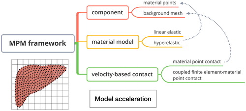
We are the first to apply MPM to needle-tissue interaction modeling, which is an extension of the particle-in-cell (PIC) from fluid mechanics into solid mechanics (Sulsky et al. 1994). Being one of the meshfree method, the MPM has been widely applied to applications such as penetration, dynamic impact and indentation (Yang et al. 2012; Li et al. 2014; Liu et al. 2016; Liang et al. 2017). An introduction flowchart is shown in Figure 1. Both the discrete material particles and background mesh existed in MPM. The continuum of a material is represented with a group of particles instead of meshes to avoid mesh tangling problem. The governing equations are solved on the structured background mesh and the information is transmitted from the particle onto mesh by appropriate mapping function. Unlike other meshless methods, the history-dependent information such as momentum and material parameters are carried on the particles. The material model is utilized to describe the relationship between strain and stress, which can be divided into two categories: linear-elastic model and hyper-elastic model. On the problem of large deformation, hyper-elastic material model is more proper since the strain-stress curves exhibit obvious non-linearity. A velocity-consistent based contact algorithm include material point method (MPM) contact and coupled finite element-material point (CFEMP) contact for needle-tissue interaction force derivation. The core ideas of the contact algorithms are the consistency of the normal velocity on the contact surface. According to this rules, the contact force can be solved. In addition, in the aim of improving the simulation efficiency, mass scaling technique is utilized.

Figure 1. Block diagram of material point method.

3. Modeling methodology

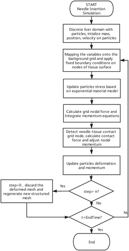
3.1. Overall algorithm flowchart (Zhang et al. 2013)

The MPM based simulation algorithm is shown in Figure 2. The history-dependent information such as material parameters, momentum is firstly initialized and stored on the material points. The mass of the particles are mapped onto the grid nodes, as in Equation (1)(1) $$m_I=\sum _p{m}_p{N}_{pI}({\mathit{x}}_p)$$(1) , (1) $$m_I=\sum _p{m}_p{N}_{pI}({\mathit{x}}_p)$$(1) where m_I is a lumped, diagonal mass matrix of the mesh node I, and it is calculated as the sum of the particle mass m_p in the element multiplying the element shape function $N_{pI}(·).$ m_p is determined by the user-defined material density and the discrete volume. The momentum of the particle is mapped onto the grid in the same way, as shown in Equation (2)(2) $$P_{Ij}=\sum _p{v}_{pj}{m}_p{N}_{pI}({\mathit{x}}_p)$$(2) , (2) $$P_{Ij}=\sum _p{v}_{pj}{m}_p{N}_{pI}({\mathit{x}}_p)$$(2) where $j\in 1,2,3$ represent the three direction in three dimensional simulation. The fixed boundary condition is applied to the nodes I on the fixed tissue surface in the direction j, of which the momentum P_ij = 0. Then particle stress is updated based on the constitutive law, i.e., The stress tensor $\sigma =f(ϵ)$ is the function of the strain tensor. The detailed mathematical expression of material model is introduced in the next section. The updated stress is mapped onto the grid nodes and integrated in the mesh volume for new nodal force. Then the momentum is updated in the time step $t+\Delta t$ as shown in Equation (3)(3) $$P_{Ij}^{t+\Delta t}=P_{Ij}^t+f_{Ij}\Delta t$$(3) . (3) $$P_{Ij}^{t+\Delta t}=P_{Ij}^t+f_{Ij}\Delta t$$(3)

Figure 2. Overall algorithm flowchart of MPM.

The momentum on each nodes is used for kinematic parameter update including the velocity v_p and position x_p on the particles in Equation (4)(4) $$\begin{array}{c}{v}_{pj}^{t+\Delta t}=v_{pj}^t+N_{Ip}\frac{f_{Ij}}{m_I}\Delta t\hfill \\ x_{pj}^{t+\Delta t}=x_{pj}^t+N_{Ip}\frac{P_{Ij}}{m_I}\Delta t\hfill \end{array}$$(4) , where N_Ip is the mapping function from mesh nodes to particles. (4) $$\begin{array}{c}{v}_{pj}^{t+\Delta t}=v_{pj}^t+N_{Ip}\frac{f_{Ij}}{m_I}\Delta t\hfill \\ x_{pj}^{t+\Delta t}=x_{pj}^t+N_{Ip}\frac{P_{Ij}}{m_I}\Delta t\hfill \end{array}$$(4)

We reset the structured mesh every n steps. It means that the deformed mesh will be discarded and the structured mesh will be regenerated every n time steps, which can effectively avoid mesh distortion and sharp decrease of time step.

3.2. The exponential material model

In this section, we establish a proper hyperelastic constitutive law to approximate the pork liver and PVA phantom, which is the functional relationship to specify the stress components in terms of strain within a nonlinear regime. Hyperelastic material postulates the existence of strain-energy function, $\Psi =\Psi (F)$ is a typical example of a scaler-valued function of the deformation gradient tensor. In this work, we choose the right Cauchy-Green tensor and the second Piola-Kichhoff stress to establish the constitutive law which is objective, as shown in Equation (5)(5) $$S=2\frac{\partial \Psi (C)}{\partial C},$$(5) (5) $$S=2\frac{\partial \Psi (C)}{\partial C},$$(5) where S is the second-Piola-Kichhoff stress and C is the Right Cauchy-Green tensor, which is related to the deformation gradient tensor F by (6) $$C=F^{T}F,$$(6) (7) $$F=\frac{\partial \mathit{x}}{\partial \mathit{X}},$$(7) where x is the spatial position at time t of a material particle with material coordinate X. When there is no deformation, F = C = U and U is the unit matrix. In this section, the exponential model (Fung-Demiray model) (Fung 1967; Demiray 1972) is applied to the material modeling of pork liver and phantom, the exponential form of the strain energy function is shown in Equation (8)(8) $$\Psi (C)=\frac{\mu }{2\gamma }[\text{exp}\hspace{0.17em}(\gamma (I_1-3))-1)],$$(8) (8) $$\Psi (C)=\frac{\mu }{2\gamma }[\text{exp}\hspace{0.17em}(\gamma (I_1-3))-1)],$$(8) where I₁ is the first principal invariant of Right Cauchy-Green tensor and μ, γ are the constant parameters of the material model. Based on Equation (8)(8) $$\Psi (C)=\frac{\mu }{2\gamma }[\text{exp}\hspace{0.17em}(\gamma (I_1-3))-1)],$$(8) , $\frac{\partial \Psi (C)}{\partial C}$ in the Equation (5)(5) $$S=2\frac{\partial \Psi (C)}{\partial C},$$(5) can be expressed as the function of the Right Cauchy-Green tensor and its principal invariants. (9) $$\frac{\partial \Psi (C)}{\partial C}=-\frac{1}{2}p{C}^{-1}+\frac{\partial \Psi (C)}{\partial I_1}\frac{\partial I_1}{\partial C}+\frac{\partial \Psi (C)}{\partial I_2}\frac{\partial I_2}{\partial C},$$(9) where $I_1=\mathit{trace}(C),I_2=[\mathit{trace}{(C)}^2-\mathit{trace}(C^2)]/2$ are the invariants of the Right Cauchy-Green tensor and $\frac{\partial I_1}{\partial C}=U,\frac{\partial I_2}{\partial C}=I_{1}U-C.$ In the exponential model shown in Equation (8)(8) $$\Psi (C)=\frac{\mu }{2\gamma }[\text{exp}\hspace{0.17em}(\gamma (I_1-3))-1)],$$(8) , the partial derivation of strain energy function to principal invariants is calculated as (10) $$\begin{array}{c}\frac{\partial \Psi (C)}{\partial I_1}=\frac{\mu }{2}[\text{exp}\hspace{0.17em}(\gamma (I_1-3))]\hfill \\ \frac{\partial \Psi (C)}{\partial I_2}=0\hfill \end{array}$$(10) p in Equation (9)(9) $$\frac{\partial \Psi (C)}{\partial C}=-\frac{1}{2}p{C}^{-1}+\frac{\partial \Psi (C)}{\partial I_1}\frac{\partial I_1}{\partial C}+\frac{\partial \Psi (C)}{\partial I_2}\frac{\partial I_2}{\partial C},$$(9) is the hydrostatic pressure which is an indeterminate Lagrange multiplier corresponding to the equilibrium equations and boundary conditions. As for incompressibility constraints, $\mathit{detF}=J\equiv 1,$ J is the determinant value of the deformation gradient tensor F and denotes the volume change from the initial frame to current frame. p is calculated as (11) $$p=\mu /|C{|}^2$$(11)

Substituting Equations (9)(9) $$\frac{\partial \Psi (C)}{\partial C}=-\frac{1}{2}p{C}^{-1}+\frac{\partial \Psi (C)}{\partial I_1}\frac{\partial I_1}{\partial C}+\frac{\partial \Psi (C)}{\partial I_2}\frac{\partial I_2}{\partial C},$$(9) and (31)(31) $$\begin{array}{c}{\sigma }_{11}=-p{\lambda }^{-1}+2{\omega }_1\lambda -2{\omega }_2{\lambda }^{-3}\hfill \\ {\sigma }_{22}=-p{\lambda }^{1/2}+2{\omega }_1{\lambda }^{-1/2}-2{\omega }_2{\lambda }^{3/2}\hfill \\ {\sigma }_{33}=-p{\lambda }^{1/2}+2{\omega }_1{\lambda }^{-1/2}-2{\omega }_2{\lambda }^{3/2}\hfill \end{array}$$(31) into Equation (5)(5) $$S=2\frac{\partial \Psi (C)}{\partial C},$$(5) , the second Piola-Kichhoff stress is updated according to the deformation tensor, as shown in Equation (12)(12) $$S=-\mu C^{-1}/|C{|}^2+\mu [\text{exp}\hspace{0.17em}(\gamma (I_1-3))])U$$(12) . The Cauchy stress can be calculated in terms of the second Piola-Kichhoff stress in Equation (13)(13) $$\sigma =J^{-1}FS{F}^T.$$(13) . (12) $$S=-\mu C^{-1}/|C{|}^2+\mu [\text{exp}\hspace{0.17em}(\gamma (I_1-3))])U$$(12) (13) $$\sigma =J^{-1}FS{F}^T.$$(13)

3.3. Needle-tissue interaction force derivation

There are two kinds of needle-tissue interaction force models: a particle to particle based material point method (MPM) contact force model and particle to element based coupled finite element-material point (CFEMP) contact force model. In MPM contact, contact is easy to implement which is solved on mesh nodes. Both needle and the whole tissue are discretized as particles which can be used to simulate the global needle-tissue interaction. But the 3 D geometry of the needle is not considered that is modeled as a row of points. In CFEMP contact, tissue is modeled as material point body, while needle is modeled as finite element body and the shape of needle tip and diameter are taken into account. CFEMP has advantages in tracking contact surface accurately. Considering the computational efficiency, only the tissue area that is near the needle trajectory is modeled. MPM contact is used to establish the global needle-tissue interaction model while CFEMP contact is used to simulate the local needle cutting process. Both the MPM contact and CFEMP contact are derived in two steps: contact nodes detection and a velocity-consistent condition based interaction force calculation.

3.3.1. MPM contact force derivation

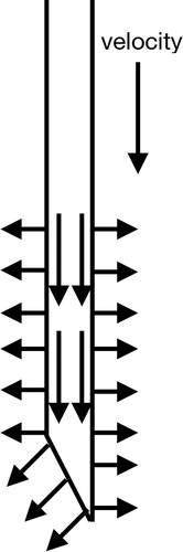
MPM contact couples two material point objects based on particle to particle contact algorithm. As can be seen in Figure 3, when needle points and the tissue points are interpolated into the same mesh node, the node is to be detected as a contact node (See yellow pentagram). The interaction force is decomposed to the normal component (the radial direction perpendicular to the cross section of the needle body) and tangential component (opposite direction of the needle velocity). Figure 4 shows the normal vector ${\mathit{n}}_i$ and tangential vector ${\mathit{t}}_i$ of the needle surface. The vectors of tissue contact surface is just opposite with that of the needle’s.

Figure 3. Contact point detection: needle points (represented as black points) and tissue points (represented as orange points) are mapped to the same background grid nodes (represented as yellow pentagram).

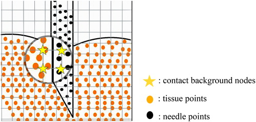
Figure 4. Normal and tangential vector of the needle surface.

The needle and tissue has contacted with each other when the velocity of needle points and tissue points meet the Equation (14)(14) $$({\mathit{v}}_{nI}-{\mathit{v}}_{tI})·{\mathit{n}}_{nI}>0,$$(14) (14) $$({\mathit{v}}_{nI}-{\mathit{v}}_{tI})·{\mathit{n}}_{nI}>0,$$(14) where ${\mathit{v}}_{nI}$ and ${\mathit{v}}_{tI}$ represent the velocity of needle points and tissue points on node I and ${\mathit{n}}_{nI}$ represents the normal vector of the contact force on node I. The velocity consistent condition requires the normal component of the velocity and acceleration of the needle and tissue on the node I should be consistent, as shown in Equations (15)(15) $${\mathit{v}}_{nI}·{\mathit{n}}_{nI}={\mathit{v}}_{tI}·{\mathit{n}}_{nI}$$(15) and (16)(16) $${\mathit{a}}_{nI}·{\mathit{n}}_{nI}={\mathit{a}}_{tI}·{\mathit{n}}_{nI}$$(16) . (15) $${\mathit{v}}_{nI}·{\mathit{n}}_{nI}={\mathit{v}}_{tI}·{\mathit{n}}_{nI}$$(15) (16) $${\mathit{a}}_{nI}·{\mathit{n}}_{nI}={\mathit{a}}_{tI}·{\mathit{n}}_{nI}$$(16)

According to the Newton’s second law, we can get (17) $$\begin{array}{c}{m}_{nI}({\mathit{a}}_{nI}·{\mathit{n}}_{nI})={\mathit{f}}_{nI}^{\text{int}}·{\mathit{n}}_{nI}+f_I^{\text{nor}}\hfill \\ m_{tI}({\mathit{a}}_{tI}·{\mathit{n}}_{tI})={\mathit{f}}_{tI}^{\text{int}}·{\mathit{n}}_{tI}+f_I^{\text{nor}}\hfill \end{array}$$(17) where m_nI and m_tI are the interpolation of needle mass and tissue mass on node I, $f_I^{\mathit{nor}}$ is the normal contact force between the two contact bodies at node I. Combining Equation (16)(16) $${\mathit{a}}_{nI}·{\mathit{n}}_{nI}={\mathit{a}}_{tI}·{\mathit{n}}_{nI}$$(16) with Equation (17)(17) $$\begin{array}{c}{m}_{nI}({\mathit{a}}_{nI}·{\mathit{n}}_{nI})={\mathit{f}}_{nI}^{\text{int}}·{\mathit{n}}_{nI}+f_I^{\text{nor}}\hfill \\ m_{tI}({\mathit{a}}_{tI}·{\mathit{n}}_{tI})={\mathit{f}}_{tI}^{\text{int}}·{\mathit{n}}_{tI}+f_I^{\text{nor}}\hfill \end{array}$$(17) , the formula of $f_I^{\mathit{nor}}$ is calculated in Equation (18)(18) $$f_I^{\text{nor}}=\frac{1}{m_{tI}+m_{nI}}(m_{tI}{\mathit{f}}_{nI}^{\text{int}}-m_{nI}{\mathit{f}}_{tI}^{\text{int}})·{\mathit{n}}_{nI}$$(18) , (18) $$f_I^{\text{nor}}=\frac{1}{m_{tI}+m_{nI}}(m_{tI}{\mathit{f}}_{nI}^{\text{int}}-m_{nI}{\mathit{f}}_{tI}^{\text{int}})·{\mathit{n}}_{nI}$$(18)

The tangential component of the contact force is related to the friction force. In needle-tissue interaction model, friction force is the most important force that dominates the force profile which is distributed along the needle body (Jiang et al. 2014). There are two status in Coulomb friction model: static and kinetic. For static regime, the two contact bodies remain sticking to each other, similar to the velocity-consistent conditions in normal component, the static friction is calculated as: (19) $$f_I^{\text{sta}}=\frac{1}{m_{tI}+m_{nI}}(m_{tI}{\mathit{f}}_{nI}^{\text{int}}-m_{nI}{\mathit{f}}_{tI}^{\text{int}})·{\mathit{t}}_{nI}$$(19) where ${\mathit{t}}_{nI}$ is the tangential vector at node I. The static friction at zero velocity can take any range of values and oppose the impending motion. Kinetic friction is a constant value that is equal to the normal force multiply by the friction coefficient μ, and the direction of kinetic friction force opposes the insertion velocity, as shown in (20) $$f_I^{\text{fric}}=\mu f_I^{\text{nor}}$$(20)

With the assumption that the maximum static friction force is equal to the kinetic friction force, the tangential component of the contact force is calculated as (21) $$f_I^{\hspace{0.17em}\text{tan}\hspace{0.17em}}=\min \{f_I^{\text{sta}},f_I^{\text{fric}}\}$$(21)

3.3.2. CFEMP contact force derivation

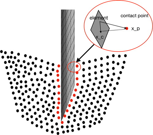
A particle-to-surface contact algorithm is employed to couple the finite element object and the material point object. The main difference between the MPM contact and CFEMP contact is the contact detection procedures: CFEMP contact searches for the contact pairs by space search methods, which is determined by the contact position and contact gap. As shown in Figure 5, assume the contact position x^c is the foot of the perpendicular of the particle x^p on to the element surface. And contact gap is the vertical distance between the particle x^p and contact location x^c, the direction of which is also consistent with the normal vector of finite element surface.

Figure 5. Schematic of the CFEMP based contact.

It is assumed that the two body have been contacted with each other when the contact gap g should satisfies that: (22) $$g<\frac{(d_e+d_p)}{2}$$(22) where d_e and d_p are the element size and particle diameter, respectively. Similar to the MPM contact force derivation, the contact condition of CFEMP contact requires the continuity of the velocity of the tissue points and contact position on the needle element in the normal direction. The contact force in the normal direction is calculated as: (23) $$f^{\mathit{nor}}=\frac{m_p^{\prime }{m}_c^{\prime }}{\Delta t(m_p^{\prime }+m_c^{\prime })}({\widehat{\mathit{v}}}^{p,k+1/2}-{\widehat{\mathit{v}}}^{c,k+1/2})·{\mathit{n}}^c$$(23) where $m_p^{\prime }$ and $m_c^{\prime }$ are the equivalent mass of the contact pairs and can be calculated as (24) $$\begin{array}{c}\frac{1}{m_p^{\prime }}=\sum _{I=1}^8\frac{N_{Ip}^2}{m_I}\hfill \\ \frac{1}{m_c^{\prime }}=\sum _{J=1}^4\frac{N_J^2}{m_J}\hfill \end{array}$$(24)

3.4. Tissue fracture in MPM

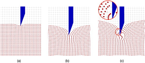
In MPM, the tissue fracture is characterized by the numerical fracture. Numerical fracture occurs when the interacted points in the same or neighbouring grid are separated into two nonadjacent grids. As can be seen in Figure 6, as the needle insertion into the internal part of tissues, the tissue points would move following the contacted needle points gradually due to the interaction force, and the distance between the surface tissue particles are enlarged, as shown in Figure 6(a,b). When the distance of the particles are stretched into two nonadjacent grids, as shown in Figure 6(c), numerical fracture occurs. Under this circumstance, the separated points would not interact with each other which means the internal force between the separated force instantly returns to zero. Then the tissue points interacted with the needle body would still follow and move into the deep of tissues while the others points would have an instantaneous springback.

Figure 6. Numerical fracture in needle insertion: the distance between the surface tissue particles are enlarged in (a) and (b), numerical fracture occurs in (c).

3.5. Model acceleration

Needle insertion can be defined as a discontinuous problem and the needle-tissue contact dominates the solution and may lead to local instability. It allows implicit solver to proceed with iterations and require a new stiffness matrix to be formed in each step which is difficult to converge. Differently for explicit integration scheme, the state at a given instant is a function of the previous time instants that can be easily implemented by avoiding the iterations of matrix inversion process. Hence, we use explicit solver for MPM needle-tissue interaction model.

However, the explicit scheme is only conditionally stable, potentially requiring very small time steps to provide an accurate and stable solution. The approximation of stability limit $\Delta t_{cr}$ is equal the smallest transit time that the stress wave across any of the elements in the mesh, as calculated in Equation (25)(25) $$\Delta t_{cr}=\underset{e}{\min }\frac{d_c}{{\max }_p(c_p+|u_p|)},$$(25) . (25) $$\Delta t_{cr}=\underset{e}{\min }\frac{d_c}{{\max }_p(c_p+|u_p|)},$$(25) where d_c is the characteristic length of the background grid. c_p and u_p are the sound material wave speed and the velocity of the particles, respectively. The time increment $\Delta t$ must be smaller than $\Delta t_{cr}$ and is calculated as (26) $$\Delta t=k_t\Delta t_{cr},$$(26) where $k_t\in [0,1]$ is time step factor. Generally, u_p is ignorable to the material wave speed c_p. c_p is determined by the material properties and density of the needle and tissues. The calculation formula of material wave speed is shown in Equation (27)(27) $$c_p=\sqrt{\frac{E(1-\nu )}{(1+\nu )(1-2\nu )\rho }}$$(27) . (27) $$c_p=\sqrt{\frac{E(1-\nu )}{(1+\nu )(1-2\nu )\rho }}$$(27) where E and ν denote the Young’s modulus and Poisson’s ratio of the material. ρ denotes the density of material point. Substituting with the needle parameters, the time step is in the order of ${10}^{-8}.$ Compared to the inherent time scale in needle insertion (range from a few to a dozen seconds), it is impractical to take the extremely large number of increments. Hence, the material parameters of the needle limits the needle-tissue interaction computation.

In minimally invasive surgery, needle insertion is normally performed at a relatively low speeds, and the inertia effects are not significant (Chanthasopeephan et al. 2003; DiMaio and Salcudean 2003; Gao et al. 2016). A potential solution is the mass scaling technique, which reduces the ratio of the event time for wave propagation across an element while leaving the event time fixed by scaling the particle mass. As can be seen in Equation (27)(27) $$c_p=\sqrt{\frac{E(1-\nu )}{(1+\nu )(1-2\nu )\rho }}$$(27) , when the mass/density is magnified c² times, the material wave speed c_p is reduced by c times; thus, the time step increment is magnified c times. When divide the numerator and denominator by m_nI in Equation (18)(18) $$f_I^{\text{nor}}=\frac{1}{m_{tI}+m_{nI}}(m_{tI}{\mathit{f}}_{nI}^{\text{int}}-m_{nI}{\mathit{f}}_{tI}^{\text{int}})·{\mathit{n}}_{nI}$$(18) , we can get the normal contact force as: (28) $$f_I^{\text{nor}}=\frac{1}{1+\frac{m_{tI}}{m_{nI}}}({\mathit{f}}_{nI}^{\text{int}}-\frac{m_{tI}}{m_{nI}}{\mathit{f}}_{tI}^{\text{int}})·{\mathit{n}}_{nI}$$(28)

In Equation (28)(28) $$f_I^{\text{nor}}=\frac{1}{1+\frac{m_{tI}}{m_{nI}}}({\mathit{f}}_{nI}^{\text{int}}-\frac{m_{tI}}{m_{nI}}{\mathit{f}}_{tI}^{\text{int}})·{\mathit{n}}_{nI}$$(28) , the mass of the tissue m_tI is far less than that of the needle m_nI. Hence, magnifying the mass of the needle would not have effects on the contact force calculation by much while improve the computational efficiency greatly.

4. Simulation of needle insertion with MPM

4.1. Acquisition of the material parameters

In this section, to demonstrate the feasibility and accuracy of the newly implemented exponential material model in the MPM framework, two different kinds of material, pork liver and PVA hydrogel are utilized, whose material parameters are obtained by performing the compression experiments. As shown in Figure 7, the force-displacement curves for uniform deformations of the tissues are used to fit a suitable mathematical model (Davies et al. 2002).

Figure 7. Compression Experiments of pork liver samples.

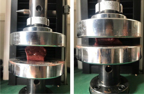
The size of pork liver and PVA phantom sample used in this work are both 18 mm × 30 mm × 30 mm. The compression speed is 1 mm/s with a maximum compression length of 5 mm. Theoretical derivation part can be regarded as a boundary-value problem, in which the vertical displacement of the tissue at the large probe is equal to the probe displacement d. The strain of the tissue is calculated by (29) $$ϵ=\frac{d}{h}$$(29) where h is the height of the tissue sample. Compression force recorded by the force sensor on the large probe is used to calculate the normal stress on the tissue top surface, (30) $${\sigma }_n=\frac{F_n}{A}$$(30) where F_n is the compression force and A is the contact area between the probe and tissues surface. The lateral friction between the tissue and probe can be neglected which means the stress on the top surface is equal to the normal stress σ_n. $\lambda =1+ϵ$ is the stretch ratio. According to the imcompressible constraints, the deformation gradient of the tissues $F=\mathit{diag}(\lambda ,{\lambda }^{-1/2},{\lambda }^{-1/2}).$

The Cauchy stress can be expressed in terms of the stretch ratio that (31) $$\begin{array}{c}{\sigma }_{11}=-p{\lambda }^{-1}+2{\omega }_1\lambda -2{\omega }_2{\lambda }^{-3}\hfill \\ {\sigma }_{22}=-p{\lambda }^{1/2}+2{\omega }_1{\lambda }^{-1/2}-2{\omega }_2{\lambda }^{3/2}\hfill \\ {\sigma }_{33}=-p{\lambda }^{1/2}+2{\omega }_1{\lambda }^{-1/2}-2{\omega }_2{\lambda }^{3/2}\hfill \end{array}$$(31)

In exponential model in Equation (8)(8) $$\Psi (C)=\frac{\mu }{2\gamma }[\text{exp}\hspace{0.17em}(\gamma (I_1-3))-1)],$$(8) , ${\omega }_1=\partial \Psi /I_1=\frac{\mu }{2}[\text{exp}\hspace{0.17em}(\gamma (I_1-3))]$ and ${\omega }_2=\partial \Psi (C)/I_2=0$ where $I_1=\mathit{trace}(F^{T}F)={\lambda }^2+2{\lambda }^{-1}.$ In the compression procedures, ${\sigma }_{22}={\sigma }_{33}=0;$ thus, the hydrostatic pressure p can be calculated as: (32) $$p=2{\omega }_1{\lambda }^{-1}-2{\omega }_2\lambda$$(32)

Substitute Equation (32)(32) $$p=2{\omega }_1{\lambda }^{-1}-2{\omega }_2\lambda$$(32) to Equation (31)(31) $$\begin{array}{c}{\sigma }_{11}=-p{\lambda }^{-1}+2{\omega }_1\lambda -2{\omega }_2{\lambda }^{-3}\hfill \\ {\sigma }_{22}=-p{\lambda }^{1/2}+2{\omega }_1{\lambda }^{-1/2}-2{\omega }_2{\lambda }^{3/2}\hfill \\ {\sigma }_{33}=-p{\lambda }^{1/2}+2{\omega }_1{\lambda }^{-1/2}-2{\omega }_2{\lambda }^{3/2}\hfill \end{array}$$(31) , the downward normal stress on the top surface is given by (33) $$\sigma =\mu ({\lambda }^{-2}-\lambda )\hspace{0.17em}\text{exp}\hspace{0.17em}(\gamma ({\lambda }^2+2{\lambda }^{-1}-3))$$(33)

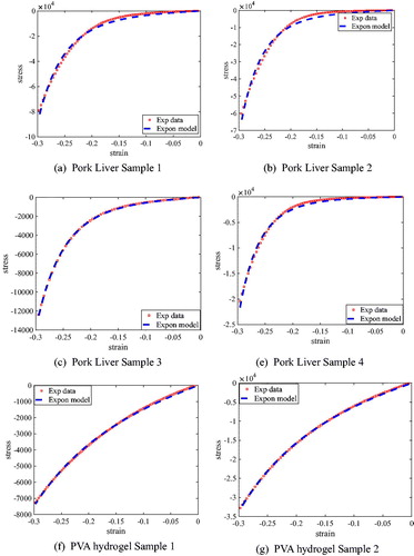
This equation indicates the stress acting on the tissues’ top surface is a function of the stretch. The exponential material parameters μ and γ can be fitted based on the least square method by applying the experimental compression data into Equation (33)(33) $$\sigma =\mu ({\lambda }^{-2}-\lambda )\hspace{0.17em}\text{exp}\hspace{0.17em}(\gamma ({\lambda }^2+2{\lambda }^{-1}-3))$$(33) . The results given in Figure 8 plots the strain-stress relationship of a couple of pork liver samples obtained from the experimental data, wherein the six pork livers samples are cut from two piece of livers. From the figure, we can conclude that there are some differences in quantitatively deviates and the nonlinear properties of pork liver from different pigs and different body parts. Figure 9 gives a couple of fitting results, where the red dotted points representing the experimental data and blue dashed line representing the fitting exponential curves are plotted together. The figure indicated that there are differences between the pork liver and PVA hydrogel. The material nonlinearity of the pork liver is more obvious than the PVA hydrogel. The compression experiments shown in Figure 9 illustrated the exponential model can be well-fitted to both pork liver and PVA hydrogel, which demonstrates the feasibility of the implemented exponential model. Based on the material model, the mechanical properties of the PVA hydrogels and pork liver can be characterized with two material parameters. The difference is due to the inherent properties from different pork liver and different gels, which can be described by the same parameters with different values.

Figure 8. Relationship of strain and stress of pork livers.

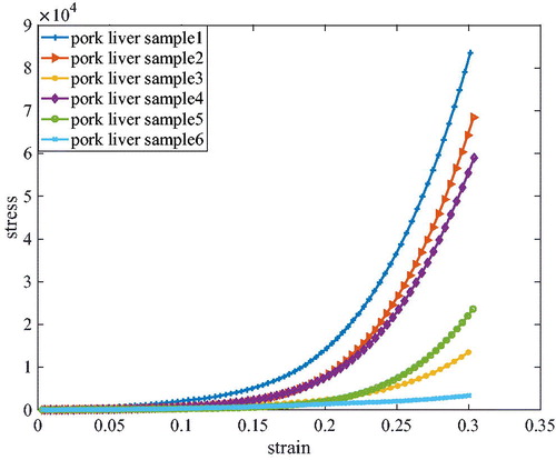
Figure 9. Comparison of exponential material model and experimental data of pork livers and PVA hydrogel.

We define the average and maximum residuals as: (34) $$\begin{array}{c}\overline{\rho }=\sum ^N|{\sigma }_{\text{fit}}-{\sigma }_{\hspace{0.17em}\text{exp}\hspace{0.17em}}|/N\hfill \\ {\rho }_{\text{max}}=\max |{\sigma }_{\text{fit}}-{\sigma }_{\hspace{0.17em}\text{exp}\hspace{0.17em}}|\hfill \end{array}$$(34) where N is the number of fitting data. The fitting results of the four samples are shown in Table 1.

Table 1. Fitting parameters of exponential material model and residuals.

Samples	μ	γ	$\overline{\rho }$	${\rho }_{\text{max}}$
Pork liver sample 1	8.71 E3	5.84	1.5 E − 3	5.30 E − 3
Pork liver sample 2	4.41 E3	7.23	1.40 E − 3	4.80 E − 3
Pork liver sample 3	1.46 E3	5.65	4.49 E − 5	2.09 E − 4
Pork liver sample 4	9.86 E2	8.39	2.70 E − 4	1.22 E − 3
PVA hydrogel sample 1	4.33 E3	0.73	4.72 E − 5	8.55 E − 5
PVA hydrogel sample 2	1.80 E4	0.95	1.35 E − 4	2.87 E − 4

As for medical needle which is made of the steel 304, Young’s modulus and Poisson’s ratio of the needle are used to determine the material wave speed. Needle is modeled as the linear elastic model that has the Young’s modulus of 2.11Gpa and Poisson’s ratio of 0.3.

4.2. MPM based global needle-tissue interaction

Global needle-tissue interaction model is established by MPM contact, which emphasizes the global tissue deformation as well as the interaction force. Instead of modeling only the local contact area, the entire tissue is modeled as a 150 mm × 100 mm × 20 mm three-dimensional cuboid structure, the size of which is the same as the PVA tissue phantom. Fixed constraints are enforced on the bottom surface of the tissue. The left and right sides are only constrained in the direction perpendicular to the needle insertion. Needle can be divided into three parts: needle base, needle body and needle tip. Due to the size differences of needle diameter and phantom, a row of points are used to represent the whole needle. The needle radial dimension and the geometry of the needle tip are not modeled. Constant velocity of 6 mm/s is enforced on the needle base nodes. The total insertion depth are 42 mm. The background mesh size is 3 mm. The particle distance of tissue is 1.5 mm while that of the needle is 5.25 mm; thus, total 37585 points are generated. The markers deformation is recorded every 3 mm of needle insertion depth.

4.3. CFEMP based local needle-tissue interaction

In this section, CFEMP is used to establish the local needle-tissue interaction where the tissue region near the needle trajectory is modeled instead of the whole tissue region. By analyzing a full size model, it was found that the stresses far from needle trajectory are negligible. As the actual 20 gauge needle has a diameter of 0.88 mm, which is far less than the tissue region. To reduce the computational burden, the model is reduced only to the interested interaction region. A sufficient modeling size of the tissue is 10 mm × 10 mm × 30 mm which is 10 times larger than the needle diameter. The model is constrained by a non-reflection boundary on front, back, left and right surfaces, setting fixed constraints on the bottom surface and leaving the top faces free to distort. Needle is discretized with finite element while tissue is discretized with particles. The needle geometry can be seen as a cylindrical body with a diameter of 0.88 mm and a 20 degree angle of the tip slope. The length of the needle is 40 mm. For high accuracy, a mesh of 8-node hexahedron solid element (SOLID164) is utilized and the needle is meshed by sweeping along the needle axis. To represent the needle radial dimension and the needle tip shape, there are 10 elements discretized along the needle external diameter and total 700 elements for the entire needle. The mesh quality analysis has been carried out on the proposed FEM model. The average aspect ratio, the average Jacobian ratio and wraping factor are 2.8027, 2.7723 and 0.014, respectively. The element size of the needle and tissue point diameters are both 0.4 mm and background mesh size is 0.8 mm. Total 49332 points are discretized for the entire interested tissue region. To extract cutting force and friction, the modeling insertion depth is 24 mm with insertion speed of 6 mm/s. The kinematic friction coefficient is 0.255 which comes from an experimental test in (Urrea et al. 2016). The exponential material model and the utilized parameters are shown in Table 1. Mass scaling factor c is 10⁴ which is tested to ensure the convergence of the results while reduces the computational burden. We choose a time step factor k_t of 0.4 to ensure the stability of the numerical model. The MPM explicit solver is established in a C++ based MPM3D, while incorporating an interface of a user-defined exponential material model.

5. Experimental verification

5.1. Experimental testbed

In medical research, simulation experiments require the use of tissue-like objects that mimic the properties of human or animal tissues, which should have similar material properties with the real tissue. Among the numerous simulation materials, PVA hydrogel have been extensively used as a phantom material to mimic the mechanical behavior of soft biological tissues. Mano et al. (2005) used an appropriate ratio of PVA and water to produce the gel which is proved to be close to human soft tissue in MRI parameters. In Jiang et al. (2011), PVA materials are adopted to substitute for real tissues in vitro to investigate the biopsy precision, and the mechanical properties of the PVA gel were also compared with the porcine liver by performing the uniaxial tests. In this paper, a transparent phantom made of Polyvinyl alcohol (PVA) hydrogel is used as a substitute for soft tissues.

The testbed of needle insertion into a PVA phantom is established and utilized to verify both the interaction force and global deformation. The experimental testbed consists of two-axis micro-displacement stages (PI Company, M-L01) for needle steering, CCD camera (MV-EM510C/M) for deformation recording, LED backlight for illumination, as shown in Figure 10. Total 12 PVA phantoms were made for validation, which can be divided into 4 groups, as shown in Table 2 and each group has three phantoms made of the same ratio of the materials; thus having the same mechanical parameters. The material parameters of each group are pre-determined by the compression experiments and recorded in Table 2, which provided the input parameters for the simulation model.

Figure 10. Experiment testbed of needle insertion into a phantom.

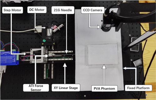
Table 2. PVA phantom parameters.

Samples	μ	γ	Size
Group 1	$4.33E3$	0.73	150 mm × 20 mm × 100 mm
Group 2	$1.80E4$	0.95	150 mm × 20 mm × 100 mm
Group 3	$4.33E3$	0.73	30 mm × 30 mm × 30 mm
Group 4	$1.80E4$	0.95	30 mm × 30 mm × 30 mm

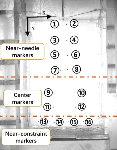
Group 1 and 2 are used for global deformation model validation while group 3 and 4 are used for CFEMP contact force validation. All of the phantom is constrained on the bottom surface. Both left side and right side can deform freely in the insertion direction. Markers are used for visualization of the phantom deformation and made in exactly the same way except for adding little ink for dyeing. There are total 16 markers buried in each phantom, as shown in Figure 11, wherein markers 1–8 represent the area near the needle insertion path while markers 13–16 denote the area near the constraints. Other markers 9–12 represent the positions in the tissue center. The markers movement recorded by the CCD camera (MV-EM510C/M) represented the deformation of the corresponding positions. The deformation results are obtained through image processing technology. The revolution of picture is 2456 × 2058 and the pixel size is up to 3.45 × 3.45 μm, the acquire frame of which is 3 pic/sec. A 20 G needle (PTC-B, Bard peripheral vascular, Inc) with a beveled tip, and the insertion velocity is $6mm/s.$ ATI force sensor of six degrees of freedom were utilized for measuring insertion force and torque.

Figure 11. Markers distribution in the PVA phantom.

5.2. Comparison of experimental and simulation results

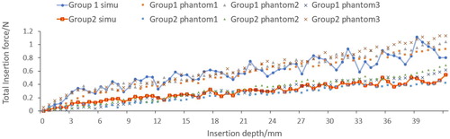
Material point method based global needle-tissue interaction validation include the interaction force validation and deformation validation. Figure 12 shows the visualization results of the strain in z direction. The total force of material point based interaction is the integral of the axial force along the needle body. The total insertion depth is 42 mm. The comparison between the simulation force and experimental data is shown in Figure 13. The phantoms in the same group exhibit similar force-displacement curves, which indicate the good experimental repeatability. Phantoms in group 2 generate larger force output than phantoms in group 1, and the fracture in group 1 occurs at 4 mm depth. The force growth rate before fracture is obviously different with that after fracture in group 2. However, fracture is not obvious in group 1 which is probably due to the softer material properties.

Figure 12. Visualization of global needle-tissue interaction based on MPM contact.

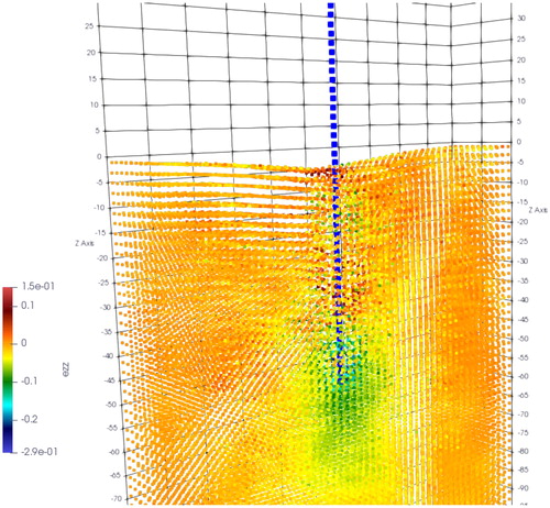
Figure 13. Comparison of MPM contact force and experimental measured force.

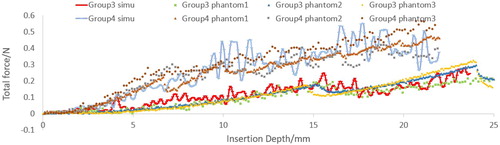
The simulation results of CFEMP are shown in Figure 14, which indicate the maximum von mises occurs at the needle tip. The total interaction force calculated from CFEMP in the insertion direction is extracted, which is the integral of the force on the needle elements in each step. The comparison with experimental data is shown in Figure 15. As can been seen from the Figure 15, due to the different stiffness of the soft phantom, fracture occurs at 15 mm in group 3 while at 6 mm in group 4, and the group 4 tends to have larger interaction force. The force growth rate with the insertion depth has obvious differences in group 4. Basically, the simulation results are consistent with the experimental data and can reflect the character of interaction force in different kinds of soft material.

Figure 14. Visualization of local CFEMP contact: the maximum von Mises occurs at the needle tip.

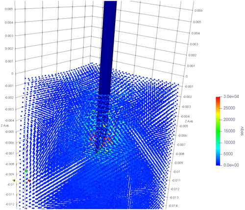
Figure 15. Comparison of CFEMP contact force and experimental measured force.

To show the accuracy of the proposed FEM model, the root mean squared error (RMSE) and mean absolute error (MAE) defined as (Illera et al. 2014; Íñiguez-Macedo et al. 2019; Somovilla-Gomez et al. 2020): (35) $$\begin{array}{c}\mathit{RMSE}=\sqrt{\frac{1}{n}\sum _{k=1}^n{(y_{k,\hspace{0.17em}\text{EXP}\hspace{0.17em}}-y_{k,\text{SIMU}})}^2}\hfill \\ \mathit{MAE}=\frac{1}{n}\sum _{k=1}^n|y_{k,\hspace{0.17em}\text{EXP}\hspace{0.17em}}-y_{k,\text{SIMU}}|\hfill \end{array}$$(35) where $y_{k,\hspace{0.17em}\text{EXP}\hspace{0.17em}}$ and $y_{k,\text{SIMU}}$ are the experimental force and the simulation force for the displacement k, respectively. Take the average force response of the three phantoms in each group as $y_{k,\text{SIMU}}.$ n is the number of the displacement discretion. Table 3 shows the RMSE and MAE errors obtained from the MPM contact and CFEMP contact algorithm. From the table, we can conclude that the accuracy of the CFEMP is higher than the MPM contact.

Table 3. Model accuracy evaluation of the MPM contact and CFEMP contact model.

Group ID	Contact model	RMSE	MAE
Group 1	MPM	0.0505	0.0416
Group 2	MPM	0.0965	0.0753
Group 3	CFEMP	0.0384	0.0300
Group 4	CFEMP	0.0626	0.0473

Both experimental data and simulation data exhibit features of small rises and drops in interaction force. However, the fluctuation amplitude in MPM is bigger than the experimental data. There are two sources that caused force fluctuation in MPM: one source is the cross-grid noise when the material points move from one grid to another when the needle inserted deep into the tissue. The other source is contributed by the lateral vibration of the contact points during the contact iteration, which may cause some contact points be detected as non-contact points. However, the fluctuation is difficult to be totally avoided because MPM is inherently a mesh-based method where structured mesh would re-regenerate and particles would move through the mesh during the iterations. To reduce the impact of fluctuation in the future, currently we are considering two potential approaches: one is to increase the density of the material points and decrease the size the background mesh grid, so that the effects of the cross-grid noise can be minimized. Another is to improve the robustness of the contact algorithm and remove high frequency noise in the force data by applying a proper filter.

The quantification of the deformation is characterized by extracting the movement of positions of markers in 20 insertion steps. The resultant deformation u_xy is defined as (36) $$u_{xy}=\sqrt{u_x^2+u_y^2}$$(36)

The maximum absolute error and the mean absolute error of the resultant deformation of 16 markers are defined as $r_{\text{max}}$ and $r_{\text{mean}},$ respectively, as shown in Equation (37)(37) $$\begin{array}{c}{r}_{\text{max}}=\underset{i=1}{\overset{16}{\max }}\left|u_{xy}^{\hspace{0.17em}\text{exp}\hspace{0.17em}}(i)-u_{xy}^{\text{simu}}(i)\right|\hfill \\ r_{\text{mean}}=\frac{1}{16}\sum _{i=1}^{16}\left|u_{xy}^{\hspace{0.17em}\text{exp}\hspace{0.17em}}(i)-u_{xy}^{\text{simu}}(i)\right|\hfill \end{array}$$(37) (37) $$\begin{array}{c}{r}_{\text{max}}=\underset{i=1}{\overset{16}{\max }}\left|u_{xy}^{\hspace{0.17em}\text{exp}\hspace{0.17em}}(i)-u_{xy}^{\text{simu}}(i)\right|\hfill \\ r_{\text{mean}}=\frac{1}{16}\sum _{i=1}^{16}\left|u_{xy}^{\hspace{0.17em}\text{exp}\hspace{0.17em}}(i)-u_{xy}^{\text{simu}}(i)\right|\hfill \end{array}$$(37) where $u_{xy}^{\hspace{0.17em}\text{exp}\hspace{0.17em}}$ and $u_{xy}^{\text{simu}}$ represent the experimental deformation and simulation deformation, respectively. Figure 16 shows $r_{\text{max}}$ and $r_{\text{mean}}$ vs insertion depth of group 1 and group 2. The maximum absolute error occurs in depth of 9 mm, which is in the rebound phase of the soft tissue. The results show the maximum error of deformation error of the resultant deformation is below 1 mm and the mean absolute error is below 0.5 mm during the whole insertion process. Tables 4 and 5 record the maximum absolute error in X direction $r_{\text{max}}^x,$ maximum absolute error in Y direction $r_{\text{max}}^y,$ mean absolute error in X direction $r_{\text{mean}}^x$ and mean absolute error in Y direction $r_{\text{mean}}^y.$

Figure 16. Maximum absolute error and the mean absolute error of the resultant deformation.

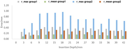
Table 4. Maximum absolute error and mean absolute error in xy direction (group 1).

Needle insertion depth/mm	$r_{\text{max}}^x$/mm	$r_{\text{max}}^y$/mm	$r_{\text{mean}}^x$/mm	$r_{\text{mean}}^y$/mm
0	0	0	0	0
0	0.00	0.00	0.00	0.00
3	0.37	0.07	0.15	0.01
6	0.57	0.06	0.15	0.02
9	0.91	0.04	0.36	0.01
12	0.93	0.10	0.26	0.02
15	0.92	0.20	0.32	0.04
18	0.95	0.17	0.30	0.03
21	0.80	0.23	0.26	0.05
24	0.69	0.15	0.29	0.05
27	0.68	0.20	0.23	0.05
30	0.72	0.18	0.28	0.07
33	0.54	0.27	0.22	0.06
36	0.56	0.52	0.28	0.06
39	0.53	0.47	0.26	0.07
42	0.44	0.54	0.25	0.09
45	0.66	0.37	0.23	0.07
48	0.63	0.38	0.25	0.08
51	0.75	0.32	0.23	0.08
54	0.72	0.29	0.25	0.08
57	0.78	0.29	0.26	0.08

Table 5. Maximum absolute error and mean absolute error in xy direction (group 2).

Needle insertion depth/mm	$r_{\text{max}}^x$/mm	$r_{\text{max}}^y$/mm	$r_{\text{mean}}^x$/mm	$r_{\text{mean}}^y$/mm
0	0.00	0.00	0.00	0.00
3	0.25	0.04	0.09	0.01
6	0.23	0.09	0.12	0.02
9	0.29	0.11	0.13	0.02
12	0.42	0.07	0.15	0.02
15	0.43	0.06	0.16	0.02
18	0.44	0.05	0.16	0.01
21	0.36	0.08	0.15	0.03
24	0.37	0.07	0.15	0.03
27	0.39	0.08	0.16	0.03
30	0.37	0.15	0.13	0.04
33	0.33	0.14	0.13	0.02
36	0.36	0.08	0.12	0.03
39	0.29	0.08	0.10	0.03
42	0.31	0.05	0.10	0.03
45	0.29	0.06	0.10	0.03
48	0.29	0.10	0.09	0.03
51	0.31	0.13	0.10	0.03
54	0.25	0.16	0.08	0.04
57	0.23	0.09	0.09	0.03

6. Conclusion and future work

In this work, novel material point method (MPM) is applied to establish the needle-tissue interaction which can avoid the difficulties including mesh distortion and adaption in traditional FEM. Given the hyperelastic material model of the soft tissue, the tissue deformation and interaction force can be solved simultaneously and independently. A testbed of needle insertion into a Polyvinyl alcohol (PVA) hydrogel is constructed to validate both tissue deformation and interaction force. Simulation results show that the experiment data agree well with the proposed model.

In the future work, the contact algorithm should be improved to avoid the cross grid noise by using a smoother shape function and the calculation efficiency should be accelerated by updating the algorithm to parallel architecture.

Disclosure statement

The authors declare that they have no conflict of interest.

Additional information

Funding

This work was supported the National Major Scientific Research Instrument Development Project of National Natural Science Foundation of China (NSFC) (Grant No. 81827804), Zhejiang Provincial Natural Science Foundation of China (grant no. LSD19H180004), Science Fund for Creative Group of NSFC (No. 51821903), and the NSFC (Grant No. 51665049).

References

- Assaad W, Jahya A, Moreira P, Misra S. 2015. Finite-element modeling of a bevel-tipped needle interacting with gel. J Mech Med Biol. 15(05):23–1210.
- Azar T, Hayward V. 2008. Estimation of the fracture toughness of soft tissue from needle insertion. In: Bello F, Edwards PJE, editors. Biomedical simulation. Berlin: Springer; p. 166–175.
- Barnett AC, Lee YS, Moore JZ. 2016. Fracture mechanics model of needle cutting tissue. J Manuf Sci Eng. 138(1):011005.
- Chanthasopeephan T, Desai JP, Lau ACW. 2003. Measuring forces in liver cutting: new equipment and experimental results. Ann Biomed Eng. 31(11):1372–1382.
- Davies PJ, Carter FJ, Alfred C. 2002. Mathematical modelling for keyhole surgery simulations: a biomechanical model for spleen tissue. Ima J Appl Math. 67(1):41–67.
- Demiray H. 1972. A note on the elasticity of soft biological tissues. J Biomech. 5(3):309–311.
- DiMaio SP, Salcudean SE. 2003. Needle insertion modeling and simulation. IEEE Trans Robot Automat. 19(5):864–875.
- Dimaio SP, Salcudean SE. 2005. Interactive simulation of needle insertion models. IEEE Trans Biomed Eng. 52(7):1167–1179.
- Fung YC. 1967. Elasticity of soft tissues in simple elongation. Am J Physiol. 213(6):1532–1544.
- Gao DD, Lei Y, Lian B, Yao B. 2016. Modeling and simulation of flexible needle insertion into soft tissue using modified local constraints. J Manuf Sci Eng. 138(12):121012.
- Gokgol C, Basdogan C, Canadinc D. 2012. Estimation of fracture toughness of liver tissue: experiments and validation. Med Eng Phys. 34(7):882–891.
- Hing JT, Brooks AD, Desai JP. 2006. Reality-based needle insertion simulation for haptic feedback in prostate brachytherapy. Proceedings - IEEE International Conference on Robotics and Automation, Orlando, FL. doi:10.1109/ROBOT.2006.1641779
- Illera M, Lostado R, Fernandez Martinez R, Mac Donald BJ. 2014. Characterization of electrolytic tinplate materials via combined finite element and regression models. J Strain Anal Eng Des. 49(6):467–480.
- Íñiguez-Macedo S, Lostado-Lorza R, Escribano-García R, Martínez-Calvo M. 2019. Finite element model updating combined with multi-response optimization for hyper-elastic materials characterization. Materials. 12(7):1019.
- Jiang S, Li P, Yu Y, Liu J, Yang Z. 2014. Experimental study of needle-tissue interaction forces: effect of needle geometries, insertion methods and tissue characteristics. J Biomech. 47(13):3344–3353.
- Jiang S, Liu S, Feng W. 2011. Pva hydrogel properties for biomedical application. J Mech Behav Biomed Mater. 4(7):1228–1233.
- Khadem M, Rossa C, Sloboda R, Usmani N, Tavakoli M. 2016. Mechanics of tissue cutting during needle insertion in biological tissue. IEEE Robot Autom Lett. 1(2):800–807.
- Kong X, Zhou P, Wu C. 2011. Numerical simulation of microneedles' insertion into skin. Comput Methods Biomech Biomed Eng. 14(9):827–835.
- Li D, Liu Y, Zhang X. 2014. Low-velocity impact responses of the stiffened composite laminated plates based on the progressive failure model and the layerwise/solid-elements method. Compos Struct. 110(1):249–275.
- Liang Y, Tamas B, Zhang X, Liu Y. 2017. Material point method with enriched shape function for crack problems. Comput Methods Appl Mech Eng. 322:541–562.
- Liu P, Liu Y, Zhang X. 2016. Simulation of hyper-velocity impact on double honeycomb sandwich panel and its staggered improvement with internal-structure model. Int J Mech Mater Des. 12(2):241–254.
- Mano I, Goshima H, Nambu M, Iio M. 2005. New polyvinyl alcohol gel material for MRI phantoms. Magn Reson Med. 3(6):921–926.
- Marchal M, Promayon E, Troccaz J. 2007. Comparisons of needle insertion in brachytherapy protocols using a soft tissue discrete model. Proceedings of the Third International Conference Surgetica 2007, Chambery, France.
- Oldfield M, Dini D, Giordano G, Rodriguez YBF. 2013. Detailed finite element modelling of deep needle insertions into a soft tissue phantom using a cohesive approach. Comput Methods Biomech Biomed Engin. 16(5):530–543.
- Ra JB, Kwon SM, Kim JK, Yi J, Kim KH, Park HW, Kyung K-U, Kwon D-S, Kang HS, Kwon ST, et al. 2002. Biomedical paper spine needle biopsy simulator using visual and force feedback. Comput Aided Surg. 7(6):353–370.
- Singh S, Lo MC, Damodaran VB, Kaplan HM, Kohn J, Zahn JD, Shreiber DI. 2016. Modeling the insertion mechanics of flexible neural probes coated with sacrificial polymers for optimizing probe design. Sensors. 16(3):330.
- Somovilla-Gomez F, Lostado-Lorza R, Corral-Bobadilla M, Escribano-Garcia R. 2020. Improvement in determining the risk of damage to the human lumbar functional spinal unit considering age, height, weight and sex using a combination of fem and rsm. Biomech Model Mechanobiol. 19(1):351–387.
- Sulsky D, Chen Z, Schreyer HL. 1994. A particle method for history-dependent materials. Comput Methods Appl Mech Eng. 118(1-2):179–196.
- Takabi B, Tai BL. 2017. A review of cutting mechanics and modeling techniques for biological materials. Med Eng Phys. 45:1–14.
- Ullrich S, Grottke O, Rossaint R, Staat M, Deserno TM, Kuhlen T. 2010. Virtual needle simulation with haptics for regional anaesthesia. IEEE Virtual Reality. 52(7):1–3.
- Urrea FA, Casanova F, Orozco GA, García JJ. 2016. Evaluation of the friction coefficient, the radial stress, and the damage work during needle insertions into agarose gels. J Mech Behav Biomed Mater. 56:98–105.
- Yang P, Liu Y, Zhang X. 2012. Simulation of fragmentation with material point method based on gurson model and random failure. Comput Model Eng Sci. 85(3):207–237.
- Zhang X, Lian Y, Liu Y, Zhou X. 2013. Material point method. Tsinghua University Press. http://www.tup.com.cn,http://www.wqbook.edu.cn.