Identification of Young’s modulus and equivalent spring constraint boundary conditions of the soft tissue with locally observed displacements for endoscopic liver surgery

Abstract

In endoscopic surgery, the surgical navigation system needs to calculate the deformation of soft tissue by biomechanical model which requires elastic properties and boundary conditions. However, patient-specific elastic parameters and boundary conditions of soft tissue are hard to measure accurately from the preoperative images, especially the boundary conditions will change during the operation due to the ligament cutting. In addition, simple boundary conditions such as fixed constraints and free-force constraints are not physically adequate to simulate the elastic effect of ligaments attached to the liver. In this paper, we present a novel method to identify the Young’s modulus and equivalent spring constraint boundary conditions of a locally observed soft tissue. Based on the spring constraint boundary condition, a two-step inverse algorithm is developed based on the finite element method (FEM) with integration of energy regularized Gauss-Newton (GN) method and ${\mathcal{l}}_1$-regularized method, which takes external forces and displacements of observable nodes as inputs. A series of numerical simulations and physical hydrogel phantom experiments were conducted. The results of simulation and physical experiments show that the Young’s modulus and equivalent spring constraint boundary conditions identified by the proposed method agree well with their setup true values.

Keywords:

• Finite element method
• unknown boundary condition
• spring constraint boundary condition
• inverse problem

1. Introduction

The surgery guidance system can improve the accuracy and safety of minimally invasive surgery (MIS) under endoscope by constructing a virtual model of the soft tissue to simulate deformation of the soft tissue (Hallet et al. 2015). Characterizing the elastic properties and boundary conditions of soft tissues plays an important role in improving the accuracy of surgical navigation system (Basdogan et al. 2001), but patient-specific information is difficult to obtain in endoscopic liver surgeries since only a partial area of the liver surface can be observed during the surgeries. Meanwhile, the ligaments in the unobservable area connected to the liver cannot be accurately determined using pre-operation imaging data, and may be subject to cut off during the preparation stage of operation after pneumoperitoneum (Machado et al. 2009). Besides, the Young’s modulus of liver is patient-specific and it is difficult to measure accurately before the operation. Hence, developing a systematic methodology to obtain patient-specific elastic parameters and boundary conditions of the soft tissues for the endoscopic surgical navigation system is dearly needed.

In literature of theoretical studies on the inverse problems, solving unknown displacement boundary conditions is a Cauchy problem and solving unknown stiffnesses of equivalent spring constraint boundary conditions is a Robin problem. Gong et al. proposed a novel coupled complex boundary method (CCBM) to stably solve the Cauchy problem which is an inverse problem with severe ill-posedness (Gong et al. 2016). Later, they proposed a method of solving a nonlinear inverse Robin problem through a linear Cauchy problem (Gong et al. 2020). However, the lack of discretization of physical constitutive equations in their proposed methods makes them difficult to be directly used in biomechanical models.

In studies on elastic parameters estimation, a conventional approach is to fabricate a sample with a standard shape for tension-compression test, which is impossible to perform on soft tissues intraoperatively. To solve this problem, Wang et al. (2011) developed a nonlinear elasto-mammography framework to identify the breast tissue properties using undeformed and deformed configurations. Simón-Allué et al. (2017) characterized the passive mechanical behavior of abdominal wall in vivo in an animal model using only external cameras. In the work of Gambarotta et al. (2005), a comprehensive experimental/numerical procedure was formulated and validated for the in vivo characterization of the mechanical properties of human skin and the simulation of reconstructive surgery. Lago et al. (2015) presented a method for in vivo characterization of biomechanical behavior of the human cornea by non-contact tonometry. A genetic heuristic search method was used to estimate the elastic parameters. However, when solving unknown elastic parameters, these methods always implicitly assume that the constraint boundary conditions are known, which is not valid for endoscopic liver surgery.

Several methods have been proposed to identify the unknown boundary conditions for the biomechanical model. I. Peterlik et al. (2014) proposed a method without prior assumption of the boundary condition types and placements to identify boundary conditions of a deformable organ with CT images. Later, R. Plantefève et al. (2014) presented a method for automatic modeling of boundary conditions in deformable anatomical structures based on a statistical atlas of CT images. These two methods are promising but they need CT images to obtain global displacements of the soft tissue during the operation, which are usually unavailable in endoscopic surgeries. Ece Ozkan et al. (Ozkan and Goksel 2018) developed a novel compliance boundary conditions (CBC) based on the spring boundary condition delivered by S. Cotin et al. (1996), which enabled a FEM model to simulate deformation under limited observation information of 3D ultrasound images. M. Morita et al. (2017, 2018) introduced a method to estimate the spatial distribution of elastic moduli over the entire elastic body from locally observed deformation patterns with known displacement constraints. M. Hajhashemkhani et al. developed an inverse algorithm based on 2D FEM model for the characterization of hyper-elastic material properties taking unknown boundary conditions into consideration (Hajhashemkhani et al. 2018). But their FEM model is a two-dimensional model without considering the boundary conditions of complex physical properties. In fact, the mechanical properties of the ligaments attached to the liver also affect the accuracy of the biomechanical model of the liver. Experiments conducted by Bosman et al. (2014) showed the modeling of ligaments playing an important role for parenchyma model. Some mechanical models of ligaments has been proposed. Kawauchi et al. (2008) developed a two-dimensional continuous model of the ligaments composed of fascicles bundle. Phillips et al. presented a finite element model of pelvis which was supported by ligamentous boundary conditions using spring elements distributed over realistic attachment sites (Phillips et al. 2007). Barrett et al. discovered a procedure of determing parameters of a simplified ligament model (Barrett and Callaghan 2018). In our previous work (Xu and Lei 2020), a novel method was proposed to identify unknown Young’s modulus and equivalent spring constraint boundary conditions. However, the input noise will seriously affect the robustness of the algorithm, and the diversity of stiffness values of equivalent spring constraint boundary conditions is not considered.

As can be seen from literatures, although many methods had been proposed to estimate elastic parameters and boundary conditions, few studies have been conducted to simultaneously solve the unknown boundary conditions with stiffness characteristics and the unknown Young’s modulus of soft tissues under locally observed displacements. Mathematical methods (Gong et al. 2016, 2020) lack of specific discretization algorithms for constitutive equations of soft tissue deformation. In the methods based on biomechanical model, some methods (Gambarotta et al. 2005; Wang et al. 2011; Lago et al. 2015; Simón-Allué et al. 2017) mainly focused on solving unknown elastic parameters while ignoring unknown boundary conditions, the others (Peterlik et al. 2014; Plantefève et al. 2014; Ozkan and Goksel 2018) required global displacements of soft tissue obtained from CT/MR or ultrasound images to identify unknown boundary conditions and elastic parameters. Moreover, the mechanical properties of the boundary, such as ligaments which would affect the accuracy of the biomechanical model (Phillips et al. 2007; Kawauchi et al. 2008; Bosman et al. 2014; Barrett and Callaghan 2018), were not modeled in these studies (Morita et al. 2017, 2018; Hajhashemkhani et al. 2018) for unknown boundary conditions.

Apparently, these aforementioned methods are not suitable to identify unknown elastic parameters and equivalent spring constraint boundary conditions of a soft tissue simultaneously during endoscopic liver surgery. Theoretically, solving many unknown parameters of different types at the same time in the case of limited observations with noise is a challenging inverse problem with strong ill-posedness. Therefore, a systematic approach to simultaneously estimate unknown Young’s modulus and boundary conditions of the biomechanical model still needs to be developed for endoscopic liver surgery.

The aim of this paper is to propose a novel method to identify Young’s modulus and equivalent spring constraint boundary conditions with locally observed displacements.

The main contributions of this paper are in two folds: First, an energy regularized GN method based on the principle of minimum deformation energy is proposed to solve the instability of displacement solutions when the unknown Young’s modulus and boundary conditions are solved simultaneously with limited and noisy observations. Second, we transform the physical constitutive equations of the soft tissue into the form of ${\mathcal{l}}_1$ regularization problem, so that various stiffness values of equivalent spring constraint boundary conditions can be identified with limited and noisy observations through the ${\mathcal{l}}_1$-regularized method. In this approach, spring constraint boundary conditions, as a generalization of the traditional boundary conditions, is applied to simulate elastic constraints of the soft tissue in this inverse problem. The result of this work will facilitate the construction of biomechanical models for surgical navigation and simulation systems under endoscope, which should lead to a novel framework to identify unknown Young’s modulus and boundary conditions of the soft tissue. The rest of this paper is organized as follows: Section 2 introduces the framework of the proposed method, the deduction of the two-step inverse algorithm and the design of simulation and physical experiments. In Section 3, various case studies are conducted in both simulation and physical experiments with different method compared with the proposed method to demonstrate the effectiveness of the proposed methodology. Conclusion and future work are presented in section 4.

2. Materials and methods

2.1. Framework design

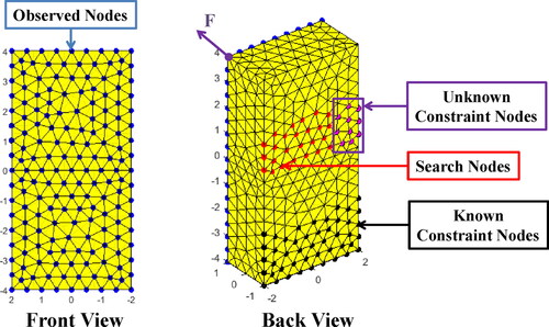
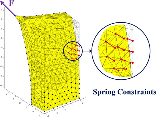
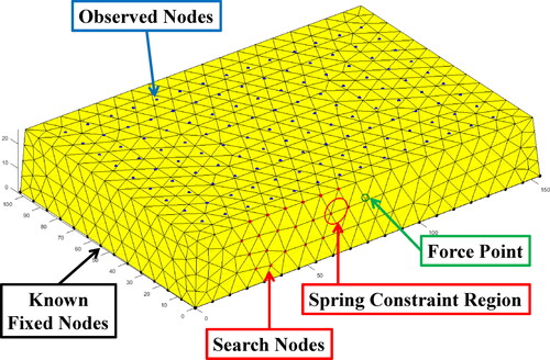
In this study, the soft tissue in endoscopic surgery is abstracted into a block for clearly illustration as shown in Figure 1. The block model consists of four main types of nodes as described below. The blue nodes on the front surface, whose number is N_o, named as observed nodes, represent observable area of the soft tissue. The red nodes on the back, whose number is N_s, named as search nodes, represent the unobservable area of the soft tissue where boundary conditions are unknown. The black nodes on the back represent the unobservable area of the soft tissue where boundary conditions can be provided by the prior knowledge. The number of all nodes in the FEM model is N_a. The pink nodes, a special kind of search nodes, named as unknown constraint nodes, represent the unobservable area where constrained boundary conditions (not free boundary conditions) are unknown. Their specific distribution and types of constraints are unknown, which are expected to estimate through the proposed method.

Figure 1. Tetrahedral FEM model for simulation experiments with various kinds of nodes.

The spring constraint boundary condition is a generalization of fixed and free constraints, which can be regarded as attaching a spring to the constrained node on the surface of a FEM model. The fixed constraint and free constraints can be captured with very large and infinitesimal spring stiffness respectively (Xu and Lei 2020). Considering the elatisity of ligaments attached to an organ, the spring constraint boundary condition is more suitable than a fixed constraint boundary condition in a soft tissue model.

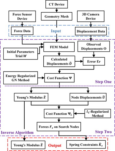
To identify the Young’s modulus and equivalent spring constraint boundary condition of the unknown area, a novel estimation framework is proposed. The flow chart of the framework is shown in Figure 2. Firstly, a tetrahedral mesh model of the object is constructed from the CT data. Secondly, special equipments with force and position sensors are used to poke the object and record the magnitude and direction of the force simultaneously. In addition, frontal surface positions are collected by endoscope or 3 D camera to calculate deformation displacement in the process. At last, the algorithm takes forces and displacements of observe nodes as inputs to calculate the Young’s modulus and the equivalent spring constraint boundary conditions.

Figure 2. Flow chart of the proposed method framework.

2.2. Two-step inverse algorithm

A two-step inverse algorithm is constructed to calculate Young’s modulus and equivalent spring constraint boundary conditions. The details of the inverse algorithm are introduced in the following two subsections.

2.2.1. Step one: Young’s modulus estimation

The displacement vector of N_o observed nodes on is expressed as $O={[u_x^{o1}{u}_y^{o1}{u}_z^{o1}\dots u_x^{o{N}_o}{u}_y^{o{N}_o}{u}_z^{o{N}_o}]}^T,$ where $u_x^{oi},u_y^{oi}$ and $u_z^{oi}$ are the displacements of the ith observe node in three direction.

The displacement vector of N_s search nodes on is expressed as $S={[u_x^{s1}{u}_y^{s1}{u}_z^{s1}\dots u_x^{s{N}_s}{u}_y^{s{N}_s}{u}_z^{s{N}_s}]}^T,$ where $u_x^{sj},u_y^{sj}$ and $u_z^{sj}$ are the displacements of the jth search node in three direction.

The iterative vector W consisting of unknown Young’s modulus E and unknown displacements of N_s search nodes is expressed as $W=[E;S].$

In each iteration, the iterative displacements (including iterative displacement vector $\widehat{O}$ of observed nodes and iterative displacement vector $\widehat{S}$ of search nodes) are updated based on FEM model, i.e. $K*U=F.$ Where K is the global stiffness based on the geometry and the Young’s modulus E of soft tissue, U is the displacement vector of all nodes and F is the force vector of external forces applied on nodes. The error between measured and calculated displacements of observed nodes is defined as $Er=O-\widehat{O}.$ Then a cost function $\Psi$ is defined as follows. (1) $$\Psi (W)=E{r}^T*Er/N_o$$(1)

Besides, a constraint function $\Phi$ is designed as a direct indicator to show the displacement error between true constraints and calculated constraints. (2) $$\Phi ={(S-\widehat{S})}^T*(S-\widehat{S})/N_s,$$(2)

A regularized Gauss-Newton (GN) method is applied in this problem for the sake of reducing the influence of observation error. The vector W is updated by minizing the value of cost function $\Psi .$ The W is updated as $W^{k+1}=W^k+D^k.$ The updated increment D for W in kth iteration is computed as follows. (3) $$D^k={[{(J^k)}^T{J}^k+\alpha ·K_R]}^{-1}[{(J^k)}^T(O-{\widehat{O}}^k)]$$(3)

In Equation (3)(3) $$D^k={[{(J^k)}^T{J}^k+\alpha ·K_R]}^{-1}[{(J^k)}^T(O-{\widehat{O}}^k)]$$(3) , I is the unit matrix, J is the sensitivity matrix, α is the regularization parameter and K_R is the regularization term. The components in J are expressed as $J_{ij}=\partial {\widehat{O}}_i/\partial W_j.$

A finite difference approximation is applied to compute the sensitivity matrix J as $J_{ij}=E{r}_i(W_j+ϵ)-E{r}_i(W_j-ϵ)/2ϵ,$where ϵ is a small increment and the cubic root of the machine number can be selected as its value (Smyl et al. 2019).

With respect to the regularization term K_R, the traditional regularization term K_I would choose the unit matrix I, i.e. K_R = I. This regularization term I reduces the effect of disturbance by making each iterative variable tend to zero. In this paper, however, we propose a new energy regularization term K_E as the regularization term, i.e. K_R = K_E. The energy regularization term is designed according to the principle of minimum deformation energy and its expression is as follows. (4) $$K_E={\widehat{U}}^T*K*\widehat{U}$$(4)

Because K_E has physical meaning, it performs better than K_I in the inverse solution of deformation problem, which is shown by subsequent simulation experiments mentioned in Section 3.1.

For the selection of regularization parameter α, the relationship between W and $\widehat{O}$ can be found. Then the iterative displacement vector $\widehat{U}$ can be calculated as follows. (5) $$\widehat{O}=M{p}_o*\widehat{U}=M{p}_o*K^{-1}*F=\underset{A}{\underbrace{M{p}_o*B}}*W$$(5)

Where Mp_o is a simple mapping matrix, i.e. $M{p}_o(i,j)={\delta }_{\widehat{i}j},$ B is a $3N_a\times (3N_s+1)$ sensitivity matrix of W to $\widehat{U},$ $\widehat{i}$ is the corresponding index number to i, i.e. $\widehat{U}(\widehat{i})=\widehat{O}(i).$

Then regularization parameter α it can be approximately determined according to the Engl’s criterion (Engl et al. 1996) as follows. (6) $$\alpha =\left|\right|A|{|}^2*{\delta }_n/((|\left|O\right||-{\delta }_n)*\left|\right|K_E\left|\right|)$$(6)

Where ${\delta }_n$ is the observation error.

Because a phenomenon called ‘semi convergence’ (Defrise and Mol 1987) will emerge when an iterative method is applied to solve the inverse problem, it is necessary to choose appropriate termination conditions for the iteration. The stopping rules of the iterative algorithm in this paper are as follows. Where k is the ordinal number of iteration.

1. $\left|\right|\widehat{O}-O\left|\right|/N_o<2\delta$

2. $({\Psi }^k-{\Psi }^{k-1})/{\Psi }^{k-1}<0.01,k>1$

2.2.2. Step two: equivalent spring constraints estimation

Assume the direction of the spring is the same direction of the displacement, the spring constraint boundary condition can be expressed as $f_i=-k_s*u_i,$ where f_i is the equivalent external force applied on the ith node, u_i is the displacement of the ith node and k_s is the spring stiffness. Then the FEM model can be reconstructed as: (7) $$\underset{\overline{K}}{\underbrace{\left[\begin{array}{ccccc}{k}_{11}& \dots & k_{1i}& \dots & k_{1N}\\ ⋮& & ⋮& & ⋮\\ k_{i1}& \dots & k_{ii}+k_s& \dots & k_{iN}\\ ⋮& & ⋮& & ⋮\\ k_{N1}& \dots & k_{Ni}& \dots & k_{NN}\end{array}\right]}}*\underset{U}{\underbrace{\left[\begin{array}{c}{u}_1\\ ⋮\\ u_i\\ ⋮\\ u_N\end{array}\right]}}=\underset{\overline{f}}{\underbrace{\left[\begin{array}{c}{f}_1\\ ⋮\\ 0\\ ⋮\\ f_N\end{array}\right]}}$$(7)

As shown in Equation (7)(7) $$\underset{\overline{K}}{\underbrace{\left[\begin{array}{ccccc}{k}_{11}& \dots & k_{1i}& \dots & k_{1N}\\ ⋮& & ⋮& & ⋮\\ k_{i1}& \dots & k_{ii}+k_s& \dots & k_{iN}\\ ⋮& & ⋮& & ⋮\\ k_{N1}& \dots & k_{Ni}& \dots & k_{NN}\end{array}\right]}}*\underset{U}{\underbrace{\left[\begin{array}{c}{u}_1\\ ⋮\\ u_i\\ ⋮\\ u_N\end{array}\right]}}=\underset{\overline{f}}{\underbrace{\left[\begin{array}{c}{f}_1\\ ⋮\\ 0\\ ⋮\\ f_N\end{array}\right]}}$$(7) , the spring constraint boundary condition could be embedded into standard FEM framework by modifing the corresponding diagonal element of stiffness matrix K.

For the inverse problem of solving the stiffness of equivalent spring boundary constraint, it can be regarded as ${\mathcal{l}}_1$-regularized least-squares problem.

The force vector F can be divided into two parts: $F=F_k+F_{uk},$ where F_k is a $3N_a\times 1$ global force vector only considering known forces obtained from the force and position sensor, and F_uk is a $3N_a\times 1$ global force vector only considering unknown forces applied to the search nodes. (8) $$F_{uk}=M{p}_F*F_s$$(8)

F_s is a $3N_s\times 1$ local force vector consisted of the force applied to search nodes and Mp_F is a $3N_a\times 3N_s$ simple mapping matrix, i.e. $M{p}_F(i,j)={\delta }_{i\widehat{j}}.$ Where $\widehat{j}$ is the corresponding index number to j, i.e. $U(\widehat{j})=S(j).$

Combined with Equations (5)(5) $$\widehat{O}=M{p}_o*\widehat{U}=M{p}_o*K^{-1}*F=\underset{A}{\underbrace{M{p}_o*B}}*W$$(5) and (8)(8) $$F_{uk}=M{p}_F*F_s$$(8) , the problem is transformed into the form of a ${\mathcal{l}}_1$ regularization problem. (9) $$\underset{A_F}{\underbrace{M{p}_o*K^{-1}*M{p}_F}}*\underset{x_F}{\underbrace{F_s}}=\underset{y_F}{\underbrace{M{p}_o*(U-K^{-1}*F_k)}}$$(9)

Then the objective function ${\Psi }_L$ of the ${\mathcal{l}}_1$ regularization problem is shown as follows. (10) $${\Psi }_L({\widehat{x}}_F)=\left|\right|A_F*{\widehat{x}}_F-y_F|{|}_2^2+\lambda |\left|{\widehat{x}}_F\right|{|}_1$$(10)

A matlab solver written by K. Koh et al. (2007) which based on a specialized iterior point method using the preconditioned conjugate gradients algorithm is applied to solve the unknown force vector F_s applied to search nodes. Then the equivalent stiffness vector $\widehat{K_s}$ can be easily calculated by the force vector F_s and displacement vector $\widehat{S},$ i.e. $\widehat{K_s}(i)=F_s(i)/\widehat{S}(i),$ where i is the index number of the node.

Where ${\widehat{x}}_F$ is the argument of regression problem and λ is the regularization parameter.

The value of λ is selected according to the method mentioned in Koh et al. (2007) as follows. (11) $$\lambda ={\delta }_n/\mathit{max}(\widehat{O})*\left|\right|2*A_F^T*y_F|{|}_{\infty }$$(11)

2.3. Experiment design

Both numerical simulation experiments and physical experiments were designed to demonstrate the feasibility of the proposed method.

2.3.1. Numerical simulation experiment design

Numerical simulation experiments were conducted on Matlab. The geometry of the object for simulation experiments was a block which was meshed into a tetrahedral FEM model as shown in Figure 1. The direct solution of displacements based on the FEM model under the set boundary conditions was taken as the true deformation. The displacements of the observed nodes and applied force were taken as inputs, the outputs were Young’s modulus and displacements of search nodes.

In the simulation experiments, the following settings were made. Fixed constraints or the spring constraints were applied to pink nodes (set as unknown) and black nodes (set as known). External force was applied to the node at the upper left corner of the block. The tetrahedral FEM model of the block consists of 937 nodes and 3956 tetrahedron elements. The number of search nodes (red and pink nodes) was 35. The number of observed nodes (blue nodes) was 171. In addition, additive white Gaussian noise (AWGN) was added into the displacements of observe nodes to simulate observation errors. The degree of noise ${\delta }_n$ was represented by SNR.

2.3.2. Physical experiment design

In the physical experiments, Polyvinyl Alcohol (PVA) hydrogel was used as a substitute for soft tissue because its Young’s modulus is controllable to possess tissue-mimicking properties by adjusting the ratio of DMSO in its mixture (Jiang et al. 2011). In this paper, a 40% DMSO PVA hydrogel was used to manufacture the phantom in physical experiments whose expected Young’s modulus was 10 kPa, which was close to the Young’s modulus of liver. The PVA hydrogel phantom was obtained by heating the PVA mixture, 32 g PVA, 160 g DMSO solvent and the 208 g de-ionized water at 140 °C for 2 hours and then frozen from room temperature to −20 °C and maintained at this temperature for 10 hours.

The size of the phantom was $100\text{mm}\times 150\text{mm}\times 25\text{mm}.$ According to the tensile test, the Young’s modulus of the 40% DMSO hydrogel phantom was in the range of $9\text{kPa}$ to $12\text{kPa}$ and the poisson’s ratio was about 0.47. It was approximately linear elastic when its strain was under 30%. Rubber bands were used to simulate the spring constraint boundary condition.

The experimental equipment included a linear two degree of freedom linear mobile platform, a six-dimensional force sensor with a force resolution of 0.0125 N and a moment resolution of 0.0625 $\mathrm{N}\mathrm{·}\text{mm}$ produced by ATI company and a micro structured light 3D depth camera with maximum observation error of 0.3 mm produced by Ailook company.

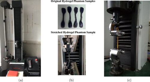
The universal tensile testing machine produced by SUNS company was used to measure the true Young’s modulus of the hydrogel phantom and the true stiffness of rubber bands. Dumbbell-shaped samples were cut from the hydrogel phantom and stretched on the universal tensile testing machine while the stress and strain are recorded by sensors. The rubber bands are clamped on the universal tensile testing machine and stretched to obtain the force-displacement curve whose slope is the demanded stiffness.

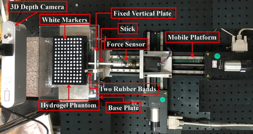
Hydrogel phantom experiments were designed as shown in Figure 3. In order to better capture the deformation of the phantom, a few drops of black ink were added to dye the hydrogel black before the step of freeze and then white markers were drawn on the surface as observed nodes. The bottom of the phantom was completely adhered to the base plate with glue. Deformation of phantom was controlled by the mobile platform through poking it with a stick. The displacements of the observation nodes on its surface were captured by the 3D depth camera and the force value was recorded by the force sensor. While simulating the elastic effect (spring constraints) of ligaments attached to the soft tissue, one end of the rubber bands was tied to a vertical fixed plate and the other end was tied to a 3D printed lightweight circular patch with 10 mm diameter glued to the phantom. The spring constraint area is set in this way because sometimes many ligaments are cut off during endoscopic liver surgery and only part of the ligaments are still attached to the liver (Machado et al. 2009).

Figure 3. Hydrogel phantom experiment.

3. Results and discussion

3.1. Numerical simulation experiments

The experimental object for simulation experiments is a $4\mathrm{m}\mathrm{\times }2\mathrm{m}\mathrm{\times }8\mathrm{m}$ block. The Young’s Modulus of the object is 10 kPa and the poisson’s ratio of the object is 0.45 which are set within the range of real elastic parameters of the liver according to Beaugrand et al. (2003). The magnitude of force applied to the top left corner of the object is 1000 N. The initial trial of the material parameters and boundary conditions are $\widehat{E}=6000\text{Pa}$ where $\widehat{E}$ denotes the iterative Young’s modulus and ${\widehat{S}}_i=[-0.5\mathrm{m},-0.5\mathrm{m},-0.5\mathrm{m}]$ where ${\widehat{S}}_i$ denotes the iterative displacements of the ith search node.

At first, fixed constraints are applied to pink nodes to test the displacement accuracy and Young’s modulus accuracy of the algorithm. The iterative displacement of node is limited in the range of −1 m to 1 m to ensure the stablility of the program.

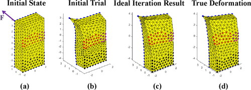
Different regularization terms (K_E and K_I) and no regularization terms were used in this series of simulation experiments under different SNR. The ideal iterative process is shown in Figure 4. Figure 4(a) shows the initial state of the object where force was applied to the top left corner of the object. Figure 4(b) shows the deformation of the object based on first guess. Figure 4(c) is the ideal final iteration result and can be compared with the true deformation shown in Figure 4(d).

Figure 4. Deformed geometries during iterative process.

The deformed geometries of experimental results are shown in Figure 5. The true displacements S and final iterative displacements $\widehat{S}$ solved by methods with different regularization terms under 40 dB SNR is illustrated in Figure 6 to compare the effects of different methods. As can be seen from the Figure 6(c), the algorithm without regularization term has not converged under the noise condition and its iterative displacements have reached the set upper and lower limits. Traditional regularization term K_I can effectively reduce the influence of noise as shown in Figure 6(b), but its effect is not as good as energy regularization term K_E as shown in Figure 6(a). The square roots of the values of the objective function $\Psi$ and constraint function $\Phi ,$ and the estimated Young’s modulus $\widehat{E}$ solved by energy regularized method are shown in Table 1. It can be seen from the table that the value of estimated Young’s modulus $\widehat{E}$ is always stable near the truth value with relative error under 2% and the constraint function $\Phi$ is less than $0.1\mathrm{m}$ in different noise conditions.

Figure 5. Deformation results under different SNR and different regularization terms.

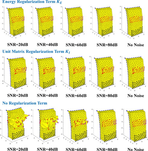
Figure 6. Results of true displacements and final iterative displacements of search nodes using different regularization terms with 40 dB SNR. (a) Energy regularization term K_E. (b) Unit matrix regularization term K_I. (c) No regularization term.

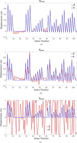
Table 1. Young’s modulus estimation results in the simulation experiments with energy regularized method.

SNR	${\Psi }^{1/2}$	${\Phi }^{1/2}$	$\widehat{E}$
20 dB	$0.1777\mathrm{m}$	$0.0882\mathrm{m}$	$10,191.75\text{Pa}$
40 dB	$0.0174\mathrm{m}$	$0.0456\mathrm{m}$	$9833.79\text{Pa}$
60 dB	$0.0025\mathrm{m}$	$0.0195\mathrm{m}$	$9996.44\text{Pa}$
80 dB	$1.87\times {10}^{-4}\mathrm{m}$	$0.0052\mathrm{m}$	$10,000.95\text{Pa}$
No noise	$1.48\times {10}^{-15}\mathrm{m}$	$5.26\times {10}^{-13}\mathrm{m}$	$10,000.00\text{Pa}$

Then each fixed constraint on the pink nodes was replaced by with the spring constraint, whose stiffness was 500 N/m, to test the stiffness accuracy of spring constraints in algorithm. The direct method, which calculates the equivalent stiffness ${\widehat{K}}_s$ by solving the forces ${\widehat{F}}_c$ directly from the FEM model, i.e. ${\widehat{F}}_c=M{p}_F^T*K^{-1}*\widehat{U},$ is also applied to compare with the ${\mathcal{l}}_1$-regularized method.

The deformation of the object based on FEM model is shown in Figure 7 whose displacements are taken as the true displacements for simulation experiments. It can be seen from the Figure 7 that the constraint nodes have displaced from the original position, which are different from the fixed constraints.

Figure 7. Deformation under spring constraints.

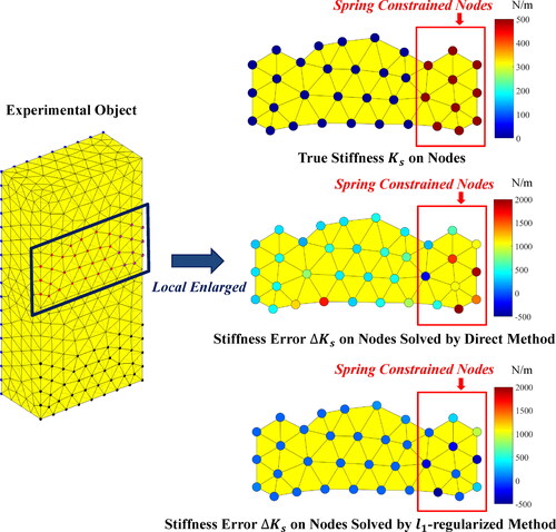
The equivalent stiffness values ${\widehat{K}}_s$ of search nodes and the stiffness errors $\Delta K_s$ ($\Delta K_s={\widehat{K}}_s-K_s$) on nodes under 40 dB SNR are illustrated in Figure 8. The color of the nodes in the figure represents the stiffness value. As can be seen from figure, the error of stiffness value solved by direct method is large at all nodes. On the contrary, the error of stiffness value solved by ${\mathcal{l}}_1$-regularized method is zero on most nodes and relatively large on spring constrained nodes. The relatively large stiffness error of ${\mathcal{l}}_1$-regularized method can be reasonably explained below.

Figure 8. Stiffness error $\Delta K_s$ on nodes solved by different method under 40 dB SNR in simulation experiments.

To explain this phenomenon, two variables ${\Gamma }_K$ and ${\Upsilon }_K$ are defined. ${\Gamma }_K$ is the sum of the stiffness of all spring constraint nodes. ${\Upsilon }_K$ is the sum of the stiffness of all search nodes. It is obvious that the true values of ${\Gamma }_K$ and ${\Upsilon }_K$ are both 5000 N/m. The ${\Gamma }_K$ and ${\Upsilon }_K$ values of results solved by different methods are shown in Table 2.

Table 2. Equivalent stiffness estimation results in the simulation experiments of spring constraint estimation.

SNR	Method	${\Gamma }_K$	${\Upsilon }_K$
20 dB	${\mathcal{l}}_1$	$4251.30\mathrm{N}/\mathrm{m}$	$5068.37\mathrm{N}/\mathrm{m}$
40 dB	${\mathcal{l}}_1$	$4971.78\mathrm{N}/\mathrm{m}$	$5315.82\mathrm{N}/\mathrm{m}$
60 dB	${\mathcal{l}}_1$	$5433.51\mathrm{N}/\mathrm{m}$	$5506.09\mathrm{N}/\mathrm{m}$
80 dB	${\mathcal{l}}_1$	$5183.22\mathrm{N}/\mathrm{m}$	$5508.13\mathrm{N}/\mathrm{m}$
No noise	${\mathcal{l}}_1$	$5000.00\mathrm{N}/\mathrm{m}$	$5000.00\mathrm{N}/\mathrm{m}$
20 dB	Direct	$3863.32\mathrm{N}/\mathrm{m}$	$8401.19\mathrm{N}/\mathrm{m}$
40 dB	Direct	$16157.13\mathrm{N}/\mathrm{m}$	$28,732.06\mathrm{N}/\mathrm{m}$
60 dB	Direct	$11,095.98\mathrm{N}/\mathrm{m}$	$16,740.04\mathrm{N}/\mathrm{m}$
80 dB	Direct	$5239.30\mathrm{N}/\mathrm{m}$	$7257.12\mathrm{N}/\mathrm{m}$
No noise	Direct	$5000.00\mathrm{N}/\mathrm{m}$	$5000.00\mathrm{N}/\mathrm{m}$

Combined with the Figure 8 and Table 2, it can be seen that ${\Gamma }_K$ and ${\Upsilon }_K$ calculated by ${\mathcal{l}}_1$-regularized method were approximated to the true value. Those smaller stiffness values can be understood as their values are added to constraint nodes with larger stiffness values and this equivalence has little effect on the FEM model. Conversely, the results obtained by direct method are poor under low SNR. The values of ${\Gamma }_K$ and ${\Upsilon }_K$ differ considerably, which means that large stiffness values also occur on unconstrained nodes and this result of direct method is clearly incorrect. Sometimes we cannot even distinguish where the constrained area is from results of direct method.

The results of the above simulation experiments show that the proposed two-steps inverse algorithm is effective.

3.2. Physical experiments

The true Young’s modulus of the hydrogel phantom and the true stiffness of the rubber bands were measured by universal tensile testing machine as shown in Figure 9. Dumbbell-shaped samples cut from the hydrogel phantom and two rubber bands were held and stretched on the universal tensile testing machine respectively. The true Young’s modulus of the phantom measured by the experiments was 10,514.54 Pa. The true stiffness value of the two rubber bands was $124.30\mathrm{N}/\mathrm{m}.$

Figure 9. Elastic parameters test experiments with universal tensile testing machine. (a) Universal tensile testing machine. (b) Original and stretched hydrogel phantom samples. (c) Stretched rubber bands.

At first, rubber bands were not used to test the displacement and Young’s modulus estimation accuarcy of the algorithm in physical experiments as shown in Figure 12(a). The CT image of hydrogel phantom is shown in Figure 10. The picture of hydrogel phantom is shown in Figure 11(a) and the tetrahedral FEM model of the hydrogel phantom, which consists of 1505 nodes and 6415 elements, is shown in Figure 11(b).

Figure 10. CT image of the hydrogel phantom.

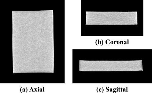
Figure 11. Hydrogel phantom and its tetrahedral FEM model. (a) Hydrogel phantom. (b) Tetrahedral FEM model with set boundary conditions.

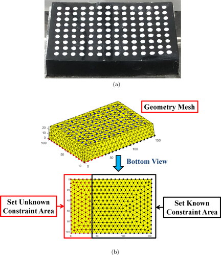
Following settings were made for algorithm. The constraints of red nodes in the red box at the bottom of the model were set as unknown and the constraints of black nodes in the black box were set as known. The blue nodes represented white markers on the hydrogel phantom. The red nodes were selected as search nodes. The number of observed nodes was 126 and the number of search nodes was 255.

The initial iterative Young’s modulus $\widehat{E}$ was set to 10,000 Pa and the intial displacement of ith search node was set as ${\widehat{S}}_i=[0.1\text{mm},0.1\text{mm},0.1\text{mm}].$

Five groups of force with different magnitudes were used to produce different deformations of the phantom for the sake of testing the performance of the algorithm under different strains. The square roots of cost function $\Psi$ and constraint function $\Phi$ as well as estimated Young’s modulus $\widehat{E}$ are illustrated in Figure 13.

The mean value of the square root of cost function $\Psi$ is 0.2718 mm. The mean value of square root of constraint function $\Phi$ is 0.2247 mm. The mean value of calculated Young’s modulus $\widehat{E}$ is 9425.18 Pa. Compared with the Young’s modulus measured by universal tensile testing machine, the relative error of Young’s modulus is 10.36%.

This error may occur for the following reasons. First, there is a small gap between the geometry of the FEM model and the real phantom, because the mesh cannot be very fine. Second, because we used the linear elastic FEM model. In several physical experiments, the deformation of the phantom is slightly large, which may not be very compatible with the small deformation assumption of the linear elastic model. The last and most important reason is that due to the limitation of equipment, the observation error itself may be close to 10%. Since the displacements of the observed nodes were only a few millimeters in experiments and the maximum observation error of depth camera was 0.3 mm, the relative errors of the input information were round 10%. According to the mathematical theory of inverse problem mentioned in Barton and Lanczos (1963); Hong and Zongyi (1994), the approximate solution cannot be more accurate than the provided original data.

Therefore, due to the observation error of about 10%, we can no longer require the final inverse solution of the algorithm to be less than 10% and the results of this algorithm were acceptable.

It can be seen from Figure 13 that the values of ${\Psi }^{1/2}$ and ${\Phi }^{1/2}$ as well as estimated Young’s modulus $\widehat{E}$ increase slightly when the magnitude of applied force increases. This phenomenon occur maybe because the linear FEM model used in the algorithm could not perfectly simulate the true deformation when the strain became large. Although the property of the PVA hydrogel phantom is close to linear elasticity, its young’s modulus will still increases slightly when the strain is large.

Then two rubber bands were used to test the stiffness accuracy of spring constraint of algorithm in physical experiments as shown in Figure 12(b). The boundary conditions for FEM model of phantom in this series of experiments are shown in Figure 14. The red circle indicates where the patch was glued to the phantom. It should be noted that this location is unknown for the algorithm.

Figure 12. Deformation of phantom under different constraints. (a) Deformation of phantom without spring constraint. (b) Deformation of phantom with spring constraint produced by two rubber bands.

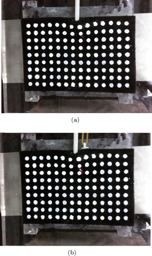
Figure 13. Results solved by the algorithm of Young’s modulus estimation with different magnitudes of force.

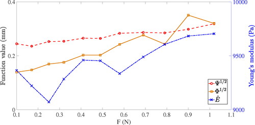
Figure 14. Boundary conditions for FEM model of phantom.

The true stiffness K_s and the stiffness error $\Delta K_s$ on nodes with spring constraint when the magnitude of external force is $5N$ are illustrated in Figure 15. Equivalent stiffness estimation results of all five groups of experiments are shown in Table 3. The mean calculated equivalent stiffness of spring constraints simluated with two rubber bands in the constraint area was $120.51\mathrm{N}/\mathrm{m}$ and the relative error of stiffness was 3.04%. In combination with Figure 15 and Table 3, although the stiffness values are concentrated on several nodes in the search area, the sum of stiffness value within the entire search area ${\Gamma }_K$ are close to the true value, and the stiffness values of the nodes outside the search area are 0 since ${\Gamma }_K$ is equal to ${\Upsilon }_K.$ Such calculated stiffness values on search nodes can be approximately equivalent to simulate the true spring constraints.

Figure 15. True stiffness K_s and stiffness error $\Delta K_s$ on nodes with spring constraint in hydrogel phantom experiments.

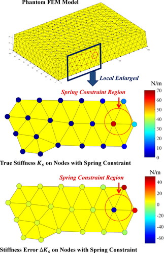
Table 3. Equivalent stiffness estimation results in the hydrogel phantom experiments of spring constraint estimation.

External force F	${\Gamma }_K$	${\Upsilon }_K$
$0.50\mathrm{N}$	$122.48\mathrm{N}/\mathrm{m}$	$122.48\mathrm{N}/\mathrm{m}$
$0.61\mathrm{N}$	$118.47\mathrm{N}/\mathrm{m}$	$118.47\mathrm{N}/\mathrm{m}$
$0.84\mathrm{N}$	$125.68\mathrm{N}/\mathrm{m}$	$125.68\mathrm{N}/\mathrm{m}$
$0.97\mathrm{N}$	$118.84\mathrm{N}/\mathrm{m}$	$118.84\mathrm{N}/\mathrm{m}$
$1.12\mathrm{N}$	$117.07\mathrm{N}/\mathrm{m}$	$117.07\mathrm{N}/\mathrm{m}$

4. Conclusion

In this paper, a novel method for identification of unknown Young’s modulus and equivalent spring constraint boundary conditions with locally observed displacements of soft tissue is developed.

The proposed method provides a two-step inverse algorithm based on the finite element method (FEM) with integration of energy regularized Gauss-Newton (GN) method and ${\mathcal{l}}_1$-regularized method.

In order to solve the problem that the solution of displacement boundary condition is unstable with noisy input, an energy regularization term was constructed according to the principle of minimum deformation energy and applied in the inverse algorithm other than the classical regularization term. For the estimation of equivalent spring constraint boundary conditions, we transformed the physical constitutive equations into the form of ${\mathcal{l}}_1$ regularization problem and solved it by ${\mathcal{l}}_1$-regularized method. A linear elastic block with 10 kPa Young’s modulus was used as the experimental object in the simulation experiments while the 40% DMSO PVA hydrogel phantom was used as the experimental object and rubber bands were used as spring constraints In the physical experiments. Numerical simulation results show that our proposed method has advantages over the classical regularization term method.

In physcial experiments, when using a depth camera with a maximum observation error of 0.3 mm, the relative error of estimated Young’s modulus is about 10% and the estimated displacement error is about 0.3 mm. For the estimation of stiffness values of equivalent spring constraints, although the stiffness values on each constraint node cannot be accurately calculated, the sum of stiffness values of nodes in the constraint region is close to the true value with relative error under 5%.

In summary, results of simulation experiments and physical hydrogel phantom experiments show that our proposed method is feasible to estimate unknown Young’s modulus and equivalent spring constraint boundary conditions with local and noisy observations.

Future work includes extending current work to consider complex Young’s modulus distribution of the soft tissue and validation with in vivo cases.

Disclosure statement

No potential conflict of interest was reported by the authors.

Additional information

Funding

This work was supported by the National Major Scientific Research Instrument Development Project of National Natural Science Foundation of China (NSFC) (Grant No. 81827804), Zhejiang Provincial Natural Science Foundation of China (grant no. LSD19H180004), Science Fund for Creative Group of NSFC (No. 51821903).

References

- Barrett JM, Callaghan JP. 2018. A procedure for determining parameters of a simplified ligament model. J Biomech. 66:175–179.
- Barton D, Lanczos C. 1963. Linear differential operators. Biometrika. 50(3/4):555.
- Basdogan C, Ho CH, Srinivasan M. 2001. Virtual environments for medical training: graphical and haptic simulation of laparoscopic common bile duct exploration. IEEE/ASME Trans Mechatron. 6(3):269–285.
- Beaugrand M, Ziol M, Sandrin L, Fournier C, Biaggi-Frassati A, Poulet B, Trinchet JC, Mal F, Christidis C, Kazemi F. 2003. 576 Liver elasticity measurement by ultrasonic transient elastography: a new non-invasive method for assessment of liver fibrosis in chronic viral hepatitis. Hepatology. 38:438–439.
- Bosman J, Haouchine N, Dequidt J, Peterlik I, Cotin S, Duriez C. 2014. The role of ligaments: Patient-specific or scenario-specific? Lect Note Comput Sci. 8789:228–232.
- Chen H, Hou ZY. 1994. The iterated regularization with perturbed operators and noisy data. Sci China Ser A. 37(12):1409–1417.
- Cotin S, Delingette H, Ayache N. 1996. Real time volumetric deformable models for surgery simulation. Lect Notes Comput Sci. 1131:535–540.
- Defrise M, Mol C. 1987. A note on stopping rules for iterative regularization methods and filtered svd. Advances in Electronics and Electron Physics. 261–268.
- Engl H, Hanke M, Neubauer A. Regularization of inverse problems. Mathematics and its Applications (Dordrecht). Dordrecht: Kluwer Academic Publishers; 1996.
- Gambarotta L, Massab R, Morbiducci R, Raposio E, Santi P. 2005. In vivo experimental testing and model identification of human scalp skin. J Biomech. 38(11):2237–2247.
- Gong RF, Cheng XL, Han W. 2016. A coupled complex boundary method for the cauchy problem. Inverse Probl Sci Eng. 24(9):1510–1527.
- Gong RF, Yu PJ, Jin QN, Cheng XL, Han W. 2020. Solving a nonlinear inverse robin problem through a linear cauchy problem. Applicable Analysis. 99(12):2093–2114.
- Hajhashemkhani M, Hematiyan MR, Goenezen S. 2018. Identification of material parameters of a hyper-elastic body with unknown boundary conditions. J Appl Mech. 85(5):051006.
- Hallet J, Soler L, Diana M, Mutter D, Baumert TF, Habersetzer F, Marescaux J, Pessaux P. 2015. Trans-thoracic minimally invasive liver resection guided by augmented reality. J Am Coll Surg. 220(5):e55–e60.
- Heiselman JS, Clements LW, Collins JA, Weis JA, Simpson AL, Geevarghese SK, Kingham TP, Jarnagin WR, Miga MI. 2018. Characterization and correction of intraoperative soft tissue deformation in image-guided laparoscopic liver surgery. J Med Imaging (Bellingham). 5(2):0212031.
- Jiang S, Liu S, Feng W. 2011. Pva hydrogel properties for biomedical application. J Mech Behav Biomed Mater. 4(7):1228–1233.
- Kawauchi Y, Ikeura N, Hirokawa S. 2008. Finite element analysis for the ligament model. Trans JSME Ser C. 74(746):2555–2561.
- Koh K, Kim SJ, Boyd S. 2007. An interior-point method for large-scale l1-regularized logistic regression. J Mach Learn Res. 8:1519–1555.
- Lago MA, Rupérez MJ, Martínez-Martínez F, Monserrat C, Larra E, Güell JL, Peris-Martínez C. 2015. A new methodology for the in vivo estimation of the elastic constants that characterize the patient-specific biomechanical behavior of the human cornea. J Biomech. 48(1):38–43.
- Machado M, Makdissi F, Surjan R, Herman P, Teixeira A, Machado M. 2009. Laparoscopic resection of left liver segments using the intrahepatic glissonian approach. Surg Endosc. 23(11):2615–2619.
- Morita M, Nakao M, Matsuda T. 2017. Elastic modulus estimation based on local displacement observation of elastic body. In: 2017 39th Annual International Conference of the IEEE Engineering in Medicine and Biology Society (EMBC).
- Morita M, Nakao M, Matsuda T. 2018. Model-based estimation of elastic moduli by local displacement observation of an elastic body. ABE. 7:39–46.
- Ozkan E, Goksel O. 2018. Compliance boundary conditions for patient-specific deformation simulation using the finite element method. Biomed Phys Eng Exp. 4(2):025003.
- Peterlik I, Courtecuisse H, Duriez C, Cotin S. 2014. Model-based identification of anatomical boundary conditions in living tissues. In: Stoyanov D, Collins DL, Sakuma I, Abolmaesumi P, Jannin P, editors. Information processing in computer-assisted interventions. Cham: Springer International Publishing; p. 196–205.
- Phillips A, Pankaj P, Howie C, Usmani A, Simpson H. 2007. Finite element modelling of the pelvis: inclusion of muscular and ligamentous boundary conditions. Med Eng Phys. 29(7):739–748.
- Plantefève R, Peterlik I, Courtecuisse H, Trivisonne R, Radoux JP, Cotin S. 2014. Atlas-based transfer of boundary conditions for biomechanical simulation. In: Golland P, Hata N, Barillot C, Hornegger J, Howe R, editors. Medical Image Computing and Computer-Assisted Intervention – MICCAI 2014. Cham: Springer International Publishing; p. 33–40.
- Rucker DC, Wu Y, Clements LW, Ondrake JE, Pheiffer TS, Simpson AL, Jarnagin WR, Miga MI. 2014. A mechanics-based nonrigid registration method for liver surgery using sparse intraoperative data. IEEE Trans Med Imaging. 33(1):147–158.
- Simón-Allué R, Calvo B, Oberai AA, Barbone PE. 2017. Towards the mechanical characterization of abdominal wall by inverse analysis. J Mech Behav Biomed Mater. 66:127–137.
- Smyl D, Bossuyt S, Liu D. 2019. Stacked elasticity imaging approach for visualizing defects in the presence of background inhomogeneity. J Eng Mech. 145(1):06018006.
- Wang ZG, Liu Y, Wang G, Sun LZ. 2011. Nonlinear elasto-mammography for characterization of breast tissue properties. Int J Biomed Imaging. 2011(4):540820.
- Xu T, Lei Y. 2020. Identification of Young’s Modulus and equivalent spring constraint boundary conditions of the object with incomplete displacement boundary conditions.