A novel micromorphic approach captures non-locality in continuum bone remodelling

Abstract

In continuum bone remodelling, bone is considered as continuous matter on the macroscale. Motivated by i) the underlying trabecular microstructure of bone resulting in size-dependence and ii) the non-local characteristics of osteocyte mechanosensing, a novel phenomenological approach based on a micromorphic formulation is proposed. Via illustrative benchmark examples, i.e. elementary unit cube, rod-shaped bone samples, and a 3D-femur sample, the novel approach is compared to the established local formulation, and the influence of the characteristic size of the microcontinuum and the coupling between macro- and microscale deformation is analysed. Taken together, the interaction between continuum points at the macroscale and their neighbourhood is effectively captured by the micromorphic formulation thus influencing the resulting distribution of nominal bone density at the macroscale.

Keywords:

• Bone remodelling
• density growth
• micromorphic continuum
• non-locality
• finite element method

1. Introduction

Bone, as a living material, is capable of adapting its internal microstructure to mechanical loading. The trabecular structure of bone and thus the nominal (homogenised) bone density strive for a biological equilibrium (homeostasis). Consequently, nominal bone density increases when mechanically overloaded and decreases when mechanically underloaded.

It is recalled that bone is a microstructural material, thus resulting in size-dependent effects (as already remarked by Galilei (1638)). Size dependence manifests as a small bone being relatively more resistant than a large one. In order to resolve the trabeculae at the microscale, Bagge (2000) describes bone remodelling as a structural optimization task in which the stiffness of the microstructure is maximised by minimising the strain energy. However, by construction, standard local continuum approaches to phenomenological bone remodelling at the macroscale do not resolve the underlying trabecular microstructure. Kuhl and Steinmann (2003) and Kuhl (2004) have accounted for the characteristic size effect of the microstructural bone material phenomenologically by including a mass flux in the mass balance, resulting in a more uniform nominal density distribution with an increase in the corresponding mass conduction coefficient or, likewise, a relative decrease in bone size. Coelho et al. (2009) and Fernandes et al. (2012) pursued optimization of microstructural stiffness while additionally minimising the metabolic cost of bone formation. In their two-scale optimization, nominal bone density is determined at the macroscale and the trabecular microstructure is captured at the microscale. Scheiner et al. (2013) coupled a model of multiscale bone mechanics with the population kinetics of bone cells. Therein, in addition to the concentration of biological cells, biochemical factors are also considered.

Moreover, according to Haj et al. (1990) and Klein-Nulend (2010), osteocytes act as mechanosensors in the adaption process, are activated by mechanical signals, and regulate the mechanical adaptation of bone. It is conjectured since long that bone remodelling at a certain point is triggered by non-locally distributed mechanosensors in its vicinity, i.e. within an influence sphere of finite size. Indeed, already Mullender et al. (1994) proposed a non-local integral formulation in which the mechanical stimulus is computationally sampled over the neighbourhood of each continuum point, necessitating two different meshes for sampling mechanosensors and simulating bone remodelling. Recently, Park et al. (2022a, 2022b) used a spatial influence function for the influence sphere capturing the distance between osteocytes and cell-forming osteoblasts and cell-absorbing osteoclasts, respectively. Schaller et al. (2022) also provided a non-local integral framework for bone remodelling using peridynamics.

Motivated by the above observations, we here extend established phenomenological concepts of local continuum bone remodelling (Kuhl et al. 2003) by a novel micromorphic approach. Continuum bone remodelling considers bone phenomenologically as an open continuum system that can continuously exchange mass, momentum, energy, and entropy with its environment, thereby emulating the processes of bone growth or degeneration, for the local case see, e.g. Papastavrou et al. (2020a, 2020b) and Schmidt et al. (2021a, 2021b). By extending these concepts to a micromorphic formulation, see Hirschberger (2008), that is augmented by the evolution of nominal bone density to capture bone remodelling, an algorithmically straightforward implementation is proposed. It avoids the need for higher continuity requirements of the finite element approximation, as required in higher gradient approaches, and expensive neighbourhood sampling, as in integral approaches. Recall that in phenomenological continuum bone remodelling, nominal bone density is considered as an effective (homogenised) macroscopic measure of the ratio of bone mass to pore volume in the underlying trabecular microstructure. Thus, in our approach, accounting for the bone microstructure is not aimed at explicitly resolving individual trabeculae, but rather at phenomenologically capturing the emergent effect on the nominal bone density at the macroscale. Here, a characteristic length measure reflects the underlying microstructure, and a scale transition parameter penalises the deviation of the micromorphic from a higher gradient case. With these parameters, the model can be calibrated to the bone microstructure, however without explicitly resolving it. Our approach is implemented in the open-source finite element library deal.II (Bangerth et al. 2007; Arndt et al. 2022).

Taken together, micromorphic bone remodelling captures the well-accepted non-locality of bone adaption, which is physiologically motivated by the underlying heterogeneous bone microstructure as well as by spatially correlated mechanosensation and -regulation.

The structure of this contribution is as follows: The classical local and the novel micromorphic continuum bone remodelling formulation as well as the finite element setting of the latter are presented in Section 2. The micromorphic approach is then illustrated in Section 3 using numerical benchmark examples, i.e. elementary unit cube and rod-shaped bone samples, as well as a 3D femoral head. We close with a discussion and conclusion in Section 4.

2. Theoretical background

In the following, we present an approach in which the classical macroscopic formulation in bone remodelling is extended to a micromorphic formulation. Therefore, the fundamental kinematics, the theory of local and micromorphic continuum bone remodelling, and the computational implementation are introduced.

2.1. Kinematics

The kinematic description of deformation on the macroscale is presented in Section 2.1.1. Subsequently, the description of the micromorphic problem on the microscale is introduced in Section 2.1.2. For a detailed account of the latter, see also Hirschberger (2008).

2.1.1. Macroscale problem

Consider a solid body where ${\mathcal{B}}_0$ denotes the reference configuration and ${\mathcal{B}}_t$ the current configuration at time t₀ and $t\in {\mathbb{R}}_{+},$ respectively. Based on the deformation map $\mathit{\phi },$ the kinematic description is characterized through the material placement X of a physical particle in the reference configuration ${\mathcal{B}}_0$ and its spatial position x in the spatial configuration ${\mathcal{B}}_t,$ that is (1) $$\mathbf{x}=\mathit{\phi }(\mathbf{X},t):{\mathcal{B}}_0\times {\mathbb{R}}_{+}\to {\mathcal{B}}_t.$$(1)

The deformation gradient F defines the linear tangent map from the material tangent space to the spatial tangent space as (2) $$\mathbf{F}:=\text{Grad}\mathit{\phi }(\mathbf{X},t):T{\mathcal{B}}_0\to T{\mathcal{B}}_t.$$(2)

Its determinant is the Jacobian $J=\mathrm{\text{det}}\mathbf{F}>0,$ which relates the volume elements in the two configurations.

2.1.2. Microscale problem

The microscale deformation gradient $\overline{\mathbf{F}}$ represents an affine map of material points from their reference placement $\overline{\mathbf{X}}$ to their current position $\overline{\mathbf{x}}$ at the microscale and is kinematically independent of the macroscale continuum, (3) $$\overline{\mathbf{x}}=\overline{\mathbf{F}}·\overline{\mathbf{X}}.$$(3)

The gradient of the microscale deformation gradient with respect to the macroscale material placement is a third-order tensor defined by (4) $$\overline{\mathbf{G}}(\mathbf{X}):=\text{Grad}\overline{\mathbf{F}}(\mathbf{X}).$$(4)

2.2. Local continuum bone remodelling

After the basic kinematic quantities have been introduced, the description of the balance equations and the constitutive assumptions in the theory of local continuum bone remodelling follow, for details see Kuhl et al. (2003).

2.2.1. Balance equations

Since bone is a living material, the nominal density ρ₀ of the considered reference volume in ${\mathcal{B}}_0$ can evolve to describe growth or atropy. In open systems theory, mass transfer can occur so that the material density may change in response to mechanical stimulation, see Kuhl et al. (2003) and Schmidt (2022). The biological equilibrium is reached, when ${\mathcal{R}}_0=0$ and thus ${\rho }_0=\mathit{\text{const}}.$ The change in density with time, $\stackrel{.}{{\rho }_0},$ therefore corresponds to the mass source ${\mathcal{R}}_0$ such that (5) $$\stackrel{.}{{\rho }_0}={\mathcal{R}}_0.$$(5)

Here we neglect mass flux, for the reasons described in the introduction, thus it does not appear in the balance of mass. The balance of linear momentum reduces to (6) $$\text{Div}\mathbf{P}=\mathbf{0}$$(6) where P is the Piola stress tensor. As motivated in Frost (1987), Jacobs et al. (1995) and Schmidt et al. (2021b) inertial effects as well as body forces are neglected in this context, since the forces acting on human bones due to physical activity are significantly larger than those caused by gravity and do not represent the dominant stimulus.

2.2.2. Constitutive equations

In the classical continuum modelling approach, bone, being an open-pored hard tissue, is characterized by a compressible neo-Hooke energy function ${\Psi }_0^{\text{neo}},$ as proposed in Kuhl et al. (2003), weighted by the relative density ${[{\rho }_0/{\rho }_0^{\star }]}^n,$ see e.g. Carter and Hayes (1977) and Gibson and Ashby (1982), (7) $${\Psi }_0={\left[\frac{{\rho }_0}{{\rho }_0^{\star }}\right]}^n{\Psi }_0^{\text{neo}}$$(7)

with (8) $${\Psi }_0^{\text{neo}}=\frac{1}{2}\lambda {\hspace{0.17em}\mathrm{\text{ln}}\hspace{0.17em}}^{2}J+\frac{1}{2}\mu \left[\mathbf{F}:\mathbf{F}-3-2\hspace{0.17em}\mathrm{\text{ln}}\hspace{0.17em}J\right].$$(8)

However, the assumption of geometrically nonlinear continuum modelling does not necessarily mean that large deformations are to be expected, but it has the advantage of not introducing additional and non-required approximations for the kinematics. Here λ and μ are the classical Lamé parameters and ρ₀ and ${\rho }_0^{\star }$ denote the current and initial values of nominal density, respectively. The exponent n characterises the actual porosity of the bone tissue and is typically set to n = 2 for trabecular bone with low nominal density, see also Schmidt et al. (2021a). As indicated in the mass balance, we assume a mass source ${\mathcal{R}}_0$ responsible for the evolution of the density in the considered reference volume. Because bone seeks for biological equilibrium, see Harrigan and Hamilton (1993) and Harrigan and Hamilton (1994), the expression for the mass source ${\mathcal{R}}_0$ (9) $${\mathcal{R}}_0={\left[\frac{{\rho }_0}{{\rho }_0^{\star }}\right]}^{-m}{\Psi }_0-{\Psi }_0^{\mathrm{a}}$$(9) balances the weighted energy density with a reference value ${\Psi }_0^{\mathrm{a}},$ called the attractor stimulus, which can be interpreted as a target energy density. The dimensionless scalar parameter m is relevant for numerical stability (Harrigan and Hamilton 1993, 1994). In the sequel, the parameter is set to m = 3, see also Kuhl and Steinmann (2003).

2.3. Micromorphic continuum bone remodelling

In the following, the balance equations and the constitutive equations are introduced similarly to Section 2.2, however now adapted for micromorphic continuum bone remodelling.

2.3.1. Balance equations

The balance of linear momentum for the micromorphic case expands to (10) $$\begin{array}{cc}\text{Div}\mathbf{P}\hfill & =\mathbf{0},\hfill \\ \text{Div}\overline{\mathbf{Q}}-\overline{\mathbf{P}}\hfill & =\mathbf{0},\hfill \end{array}$$(10) as motivated in Hirschberger et al. (2007), where $\overline{\mathbf{P}}$ is the microscale Piola stress and $\overline{\mathbf{Q}}$ is the microscale double stress. All kinetic measures associated with the problem are summarized in Table 1. The balance of mass according to Equation 5(5) $$\stackrel{.}{{\rho }_0}={\mathcal{R}}_0.$$(5) also applies in the micromorphic case.

Table 1. Summary and definition of the utilized kinetic measures. Order refers to the order of the tensorial quantity.

Measure	Label	Order
Total energy density	${\Psi }_0$	0
Macroscale deformation map	$\mathit{\phi }$	1
Macroscale deformation gradient	$\mathbf{F}=\text{Grad}\mathit{\phi }$	2
Microscale deformation gradient	$\overline{\mathbf{F}}$	2
Macroscale Piola stress	$\mathbf{P}={\mathbf{D}}_{\mathbf{F}}{\Psi }_0$	2
Microscale Piola stress	$\overline{\mathbf{P}}={\mathbf{D}}_{\overline{\mathbf{F}}}{\Psi }_0$	2
Gradient of the microscale deformation gradient	$\overline{\mathbf{G}}=\text{Grad}\overline{\mathbf{F}}$	3
Microscale double stress	$\overline{\mathbf{Q}}={\mathbf{D}}_{\overline{\mathbf{G}}}{\Psi }_0$	3

2.3.2. Constitutive equations

In the novel micromorphic approach for continuum bone remodelling, the total energy density ${\Psi }_0$ now consists not only of the local macroscale neo-Hookean energy density ${\Psi }_0^{\text{neo}},$ see Equation (8)(8) $${\Psi }_0^{\text{neo}}=\frac{1}{2}\lambda {\hspace{0.17em}\mathrm{\text{ln}}\hspace{0.17em}}^{2}J+\frac{1}{2}\mu \left[\mathbf{F}:\mathbf{F}-3-2\hspace{0.17em}\mathrm{\text{ln}}\hspace{0.17em}J\right].$$(8) , weighted by the nominal relative density, see Equation (7)(7) $${\Psi }_0={\left[\frac{{\rho }_0}{{\rho }_0^{\star }}\right]}^n{\Psi }_0^{\text{neo}}$$(7) , as typically used in classical bone growth theory, but also includes contributions from the microscale and an additional scale-bridging contribution (11) $${\Psi }_0={\left[\frac{{\rho }_0}{{\rho }_0^{\star }}\right]}^n\left[{\Psi }_0^{\text{mac}}(\mathbf{F})+{\Psi }_0^{\text{mic}}(\overline{\mathbf{G}})+{\Psi }_0^{\text{scale}}(\mathbf{F},\overline{\mathbf{F}})\right].$$(11)

Consequently, both the local macroscale and the non-local microscale contribution are scaled by the relative density. In the following, the neo-Hookean energy density is referred to as the macroscale contribution (12) $${\Psi }_0^{\text{mac}}={\Psi }_0^{\text{neo}}.$$(12)

Moreover, as described in Hirschberger (2008) and McBride et al. (2020), a quadratic formulation for the microscale energy density is assumed (13) $${\Psi }_0^{\text{mic}}=\frac{1}{2}\mu l^2\overline{\mathbf{G}}·:\overline{\mathbf{G}}$$(13)

together with a scale-bridging contribution (14) $${\Psi }_0^{\text{scale}}=\frac{1}{2}p[\overline{\mathbf{F}}-\mathbf{F}]:[\overline{\mathbf{F}}-\mathbf{F}]$$(14) coupling the macro- and microscale deformation. Here, the internal length scale parameter l accounts for size dependence and can be interpreted as the characteristic size of the microcontinuum. For $p\to 0$ the macro- and microscale contributions are decoupled, while for $p\to \infty$ the macro- and microscale deformations are penalised to become more and more equal. For the limiting case $\overline{\mathbf{F}}\equiv \mathbf{F}$ gradient elasticity is obtained. The case p = 0 and l = 0 provides the standard problem of local continuum bone remodelling. The corresponding derivatives needed for the residual, i.e. the macroscale Piola stress, the microscale Piola stress, and the microscale double stress, are computed as follows (15) $$\begin{array}{cc}\mathbf{P}\hfill & :=\frac{\partial {\Psi }_0}{\partial \mathbf{F}}={\left[\frac{{\rho }_0}{{\rho }_0^{\star }}\right]}^n\left[\left[\left[\lambda \hspace{0.17em}\mathrm{\text{ln}}\hspace{0.17em}J-\mu \right]{\mathbf{F}}^{-t}+\mu \mathbf{F}\right]-p\left[\overline{\mathbf{F}}-\mathbf{F}\right]\right],\hfill \\ \overline{\mathbf{P}}\hfill & :=\frac{\partial {\Psi }_0}{\partial \overline{\mathbf{F}}}={\left[\frac{{\rho }_0}{{\rho }_0^{\star }}\right]}^{n}p\left[\overline{\mathbf{F}}-\mathbf{F}\right],\hfill \\ \overline{\mathbf{Q}}\hfill & :=\frac{\partial {\Psi }_0}{\partial \overline{\mathbf{G}}}={\left[\frac{{\rho }_0}{{\rho }_0^{\star }}\right]}^n\mu l^2\overline{\mathbf{G}}.\hfill \end{array}$$(15)

2.4. Computational implementation

The computational implementation of the finite element formulation is performed similar to the one for micromorphic elasticity, see McBride et al. (2020), where the system consists of two primary fields, namely the macroscale deformation $\mathit{\phi }$ and the microscale deformation gradient $\overline{\mathbf{F}}.$ If additional bone growth is considered, a third variable, the nominal density, must be taken into account as an internal variable that locally results from the time discrete residual statement of the balance of mass (16) $${\mathsf{r}}_{{\rho }_0}=\Delta {\rho }_0-\Delta t{\mathcal{R}}_0({\rho }_0,\mathbf{F},\overline{\mathbf{F}},\overline{\mathbf{G}})=0.$$(16)

The discrete balance of mass is solved at each integration point using a local Newton-Raphson iteration scheme. At each global time step, the local residual is calculated and a new density is determined. The local Newton-Raphson procedure is executed for each time step until the local residual falls below a certain tolerance value. For the sake of brevity, we refrain from indicating a new time step counter and always refer to the current time step. For a more detailed description in this regard, see Schmidt (2022). With ${\mathbf{N}}_{\mathit{\phi }}^I$ and ${\mathbf{N}}_{\overline{\mathbf{F}}}^I$ denoting vector- and tensor-valued finite element shape functions, the global residual statements follow as (17) $$\begin{array}{c}{\mathsf{R}}_{\mathit{\phi }}^I:={\int }_{{\mathcal{B}}_0}[\mathbf{P}:\text{Grad}{\mathbf{N}}_{\mathit{\phi }}^I]\mathit{\text{dV}}-{\int }_{{\Gamma }_0}{\mathbf{t}}_0·{\mathbf{N}}_{\mathit{\phi }}^I\mathit{\text{dA}}\dot{=}0\hspace{1em}\forall I\in {\mathcal{I}}_{\mathit{\phi }}\hfill \\ {\mathsf{R}}_{\overline{\mathbf{F}}}^I:={\int }_{{\mathcal{B}}_0}[\overline{\mathbf{P}}:{\mathbf{N}}_{\overline{\mathbf{F}}}^I+\overline{\mathbf{Q}}·:\text{Grad}{\mathbf{N}}_{\overline{\mathbf{F}}}^I]\mathit{\text{dV}}-{\int }_{{\Gamma }_0}{\overline{\mathbf{t}}}_0·{\mathbf{N}}_{\overline{\mathbf{F}}}^I\mathit{\text{dA}}\dot{=}0\hspace{1em}\forall I\in {\mathcal{I}}_{\overline{\mathbf{F}}}.\hfill \end{array}$$(17) where the sets ${\mathcal{I}}_{\mathit{\phi }}$ and ${\mathcal{I}}_{\overline{\mathbf{F}}}$ contain the degrees of freedom for the macro- and the microscale fields. For the solution by a global Newton-Raphson scheme, the following coupled problem $$\left[\begin{array}{cc}{\mathbf{K}}_{\mathit{\phi \phi }}& {\mathbf{K}}_{\mathit{\phi }\overline{\mathbf{F}}}\\ {\mathbf{K}}_{\overline{\mathbf{F}}\mathit{\phi }}& {\mathbf{K}}_{\overline{\mathbf{F}}\overline{\mathbf{F}}}\end{array}\right]\left[\begin{array}{c}{\mathbf{d}}_{\mathit{\phi }}\\ {\mathbf{d}}_{\overline{\mathbf{F}}}\end{array}\right]=-\left[\begin{array}{c}{\mathbf{R}}_{\mathit{\phi }}\\ {\mathbf{R}}_{\overline{\mathbf{F}}}\end{array}\right]$$ results in each global Newton iteration. The line entries of the tangent operator $\mathbf{K}$ associated with the degrees of freedom $I\in$ {${\mathcal{I}}_{\mathit{\phi }},{\mathcal{I}}_{\overline{\mathbf{F}}}$} and $J\in$ {${\mathcal{I}}_{\mathit{\phi }},{\mathcal{I}}_{\overline{\mathbf{F}}}$} follow as (18) $$\begin{array}{cc}{\left[{\mathsf{K}}_{\mathit{\phi \phi }}\right]}_{\mathit{\text{IJ}}}={\partial }_{\mathit{\phi }J}{\mathsf{R}}_{\mathit{\phi }}^I=\hfill & {\int }_{{\mathcal{B}}_0}[D_{\mathbf{F}}\mathbf{P}:\text{Grad}{\mathbf{N}}_{\mathit{\phi }}^J]:\text{Grad}{\mathbf{N}}_{\mathit{\phi }}^I\mathit{\text{dV}}\hfill \\ {\left[{\mathsf{K}}_{\mathit{\phi }\overline{\mathbf{F}}}\right]}_{\mathit{\text{IJ}}}={\partial }_{\overline{\mathbf{F}}J}{\mathsf{R}}_{\mathit{\phi }}^I=\hfill & {\int }_{{\mathcal{B}}_0}[D_{\overline{\mathbf{F}}}\mathbf{P}:{\mathbf{N}}_{\overline{\mathbf{F}}}^J]:\text{Grad}{\mathbf{N}}_{\mathit{\phi }}^I\mathit{\text{dV}}\hfill \\ {\left[{\mathsf{K}}_{\overline{\mathbf{F}}\mathit{\phi }}\right]}_{\mathit{\text{IJ}}}={\partial }_{\mathit{\phi }J}{\mathsf{R}}_{\overline{\mathbf{F}}}^I=\hfill & {\int }_{{\mathcal{B}}_0}[D_{\mathbf{F}}\overline{\mathbf{P}}:\text{Grad}{\mathbf{N}}_{\mathit{\phi }}^J]:{\mathbf{N}}_{\overline{\mathbf{F}}}^I\mathit{\text{dV}}\hfill \\ {\left[{\mathsf{K}}_{\overline{\mathbf{F}}\overline{\mathbf{F}}}\right]}_{\mathit{\text{IJ}}}={\partial }_{\overline{\mathbf{F}}J}{\mathsf{R}}_{\overline{\mathbf{F}}}^I=\hfill & {\int }_{{\mathcal{B}}_0}[D_{\overline{\mathbf{F}}}\overline{\mathbf{P}}:{\mathbf{N}}_{\overline{\mathbf{F}}}^J]:{\mathbf{N}}_{\overline{\mathbf{F}}}^I\mathit{\text{dV}}\hfill \\ +\hfill & {\int }_{{\mathcal{B}}_0}[D_{\overline{\mathbf{G}}}\overline{\mathbf{Q}}·:\text{Grad}{\mathbf{N}}_{\overline{\mathbf{F}}}^J]·:\text{Grad}{\mathbf{N}}_{\overline{\mathbf{F}}}^I\mathit{\text{dV}}.\hfill \end{array}$$(18)

For quadratic convergence of the Newton-Raphson scheme, the algorithmic update of the nominal density, see Equation 16(16) $${\mathsf{r}}_{{\rho }_0}=\Delta {\rho }_0-\Delta t{\mathcal{R}}_0({\rho }_0,\mathbf{F},\overline{\mathbf{F}},\overline{\mathbf{G}})=0.$$(16) , is considered in the linearisations (19) $$\begin{array}{cc}{D}_{\mathbf{F}}\mathbf{P}\hfill & ={\partial }_{\mathbf{F}}\mathbf{P}+{\partial }_{{\rho }_0}\mathbf{P}\otimes {\delta }_{{\rho }_0}{\partial }_{\mathbf{F}}{\mathcal{R}}_0\hfill \\ D_{\overline{\mathbf{F}}}\mathbf{P}\hfill & ={\partial }_{\overline{\mathbf{F}}}\mathbf{P}+{\partial }_{{\rho }_0}\mathbf{P}\otimes {\delta }_{{\rho }_0}{\partial }_{\overline{\mathbf{F}}}{\mathcal{R}}_0\hfill \\ D_{\mathbf{F}}\overline{\mathbf{P}}\hfill & ={\partial }_{\mathbf{F}}\overline{\mathbf{P}}+{\partial }_{{\rho }_0}\overline{\mathbf{P}}\otimes {\delta }_{{\rho }_0}{\partial }_{\mathbf{F}}{\mathcal{R}}_0\hfill \\ D_{\overline{\mathbf{F}}}\overline{\mathbf{P}}\hfill & ={\partial }_{\overline{\mathbf{F}}}\overline{\mathbf{P}}+{\partial }_{{\rho }_0}\overline{\mathbf{P}}\otimes {\delta }_{{\rho }_0}{\partial }_{\overline{\mathbf{F}}}{\mathcal{R}}_0\hfill \\ D_{\overline{\mathbf{G}}}\overline{\mathbf{Q}}\hfill & ={\partial }_{\overline{\mathbf{G}}}\overline{\mathbf{Q}}+{\partial }_{{\rho }_0}\overline{\mathbf{Q}}\otimes {\delta }_{{\rho }_0}{\partial }_{\overline{\mathbf{G}}}{\mathcal{R}}_0\hfill \end{array}$$(19)

with the abbreviation (20) $${\delta }_{{\rho }_0}=\Delta t{[1-\Delta t{\partial }_{{\rho }_0}{\mathcal{R}}_0]}^{-1}.$$(20)

The entries ${\partial }_{{\rho }_0}\mathbf{P},{\partial }_{\mathbf{F}}{\mathcal{R}}_0$ and ${\partial }_{{\mathbf{\rho }}_{\mathbf{0}}}{\mathcal{R}}_0$ are defined in Kuhl and Steinmann (2003) and are provided here in the Appendix. In the same fashion, we determine the derivatives that result from the microscale deformation. Considering the constitutive equations given in Section 2.2 and 2.3, the following expressions (21) $$\begin{array}{cc}{\partial }_{\mathbf{F}}\mathbf{P}\hfill & ={\left[\frac{{\rho }_0}{{\rho }_0^{\star }}\right]}^n\left[\mu \mathbf{I}\overline{\otimes }\mathbf{I}+\lambda {\mathbf{F}}^{-t}\otimes {\mathbf{F}}^{-t}-\left[\lambda \hspace{0.17em}\mathrm{\text{ln}}\hspace{0.17em}J-\mu \right]{\mathbf{F}}^{-t}\underset{¯}{\otimes }{\mathbf{F}}^{-1}+p\mathbf{I}\overline{\otimes }\mathbf{I}\right]\hfill \\ {\partial }_{\overline{\mathbf{F}}}\mathbf{P}\hfill & ={\partial }_{\mathbf{F}}\overline{\mathbf{P}}=-{\partial }_{\overline{\mathbf{F}}}\overline{\mathbf{P}}=-p{\left[\frac{{\rho }_0}{{\rho }_0^{\star }}\right]}^n\left[\mathbf{I}\overline{\otimes }\mathbf{I}\right]\hfill \\ {\partial }_{\overline{\mathbf{G}}}\overline{\mathbf{Q}}\hfill & =\mu l^2{\left[\frac{{\rho }_0}{{\rho }_0^{\star }}\right]}^n\left[\mathbf{I}\overline{\otimes }\mathbf{I}\right]\hfill \\ {\partial }_{{\rho }_0}\overline{\mathbf{P}}\hfill & =\frac{1}{{\rho }_0}n\overline{\mathbf{P}}\hfill \\ {\partial }_{{\rho }_0}\overline{\mathbf{Q}}\hfill & =\frac{1}{{\rho }_0}n\overline{\mathbf{Q}}\hfill \\ {\partial }_{\overline{\mathbf{F}}}{\mathcal{R}}_0\hfill & ={\left[\frac{{\rho }_0}{{\rho }_0^{\star }}\right]}^{-m}\overline{\mathbf{P}}\hfill \\ {\partial }_{\overline{\mathbf{G}}}{\mathcal{R}}_0\hfill & ={\left[\frac{{\rho }_0}{{\rho }_0^{\star }}\right]}^{-m}\overline{\mathbf{Q}}\hfill \end{array}$$(21) are obtained to determine the tangent operator, given in Equation (18)(18) $$\begin{array}{cc}{\left[{\mathsf{K}}_{\mathit{\phi \phi }}\right]}_{\mathit{\text{IJ}}}={\partial }_{\mathit{\phi }J}{\mathsf{R}}_{\mathit{\phi }}^I=\hfill & {\int }_{{\mathcal{B}}_0}[D_{\mathbf{F}}\mathbf{P}:\text{Grad}{\mathbf{N}}_{\mathit{\phi }}^J]:\text{Grad}{\mathbf{N}}_{\mathit{\phi }}^I\mathit{\text{dV}}\hfill \\ {\left[{\mathsf{K}}_{\mathit{\phi }\overline{\mathbf{F}}}\right]}_{\mathit{\text{IJ}}}={\partial }_{\overline{\mathbf{F}}J}{\mathsf{R}}_{\mathit{\phi }}^I=\hfill & {\int }_{{\mathcal{B}}_0}[D_{\overline{\mathbf{F}}}\mathbf{P}:{\mathbf{N}}_{\overline{\mathbf{F}}}^J]:\text{Grad}{\mathbf{N}}_{\mathit{\phi }}^I\mathit{\text{dV}}\hfill \\ {\left[{\mathsf{K}}_{\overline{\mathbf{F}}\mathit{\phi }}\right]}_{\mathit{\text{IJ}}}={\partial }_{\mathit{\phi }J}{\mathsf{R}}_{\overline{\mathbf{F}}}^I=\hfill & {\int }_{{\mathcal{B}}_0}[D_{\mathbf{F}}\overline{\mathbf{P}}:\text{Grad}{\mathbf{N}}_{\mathit{\phi }}^J]:{\mathbf{N}}_{\overline{\mathbf{F}}}^I\mathit{\text{dV}}\hfill \\ {\left[{\mathsf{K}}_{\overline{\mathbf{F}}\overline{\mathbf{F}}}\right]}_{\mathit{\text{IJ}}}={\partial }_{\overline{\mathbf{F}}J}{\mathsf{R}}_{\overline{\mathbf{F}}}^I=\hfill & {\int }_{{\mathcal{B}}_0}[D_{\overline{\mathbf{F}}}\overline{\mathbf{P}}:{\mathbf{N}}_{\overline{\mathbf{F}}}^J]:{\mathbf{N}}_{\overline{\mathbf{F}}}^I\mathit{\text{dV}}\hfill \\ +\hfill & {\int }_{{\mathcal{B}}_0}[D_{\overline{\mathbf{G}}}\overline{\mathbf{Q}}·:\text{Grad}{\mathbf{N}}_{\overline{\mathbf{F}}}^J]·:\text{Grad}{\mathbf{N}}_{\overline{\mathbf{F}}}^I\mathit{\text{dV}}.\hfill \end{array}$$(18) .

3. Numerical examples

The presented finite element problem is solved within the open-source library deal.II (Bangerth et al. 2007; Arndt et al. 2022). It is a C++ software library that supports the creation of finite element codes for a broad variety of PDEs (Bangerth et al. 2022). For the finite element implementation we use 3D elements with a 3 × 3 quadrature rule and a tri-quadratic approximation for the macroscale deformation $\mathit{\phi }$ and a tri-linear approximation for the microscale deformation gradient $\overline{\mathbf{F}}.$

In this section, the micromorphic approach is compared with the classical approach, which will be referred to as the local approach in the following. Moreover, variations of the characteristic length scale parameter l and the penalty parameter p are performed. As a first numerical example, we consider a unit cube under inhomogeneous loading, then we study a cantilever beam representing a bone specimen of the femoral shaft, and finally we illustrate the emerged findings by calculations on a full femoral head model.

3.1. Unit cube

In order to perform basic investigations of our model, a unit cube consisting of only one finite element is considered. The dimensionless parameters used in the model are given in Table 2.

Table 2. Non-dimensionalised reference parameters for the unit cube.

Shear modulus	$\hspace{1em}\mu$	1
Poisson’s ratio	$\hspace{1em}\nu$	0.2
Initial density	$\hspace{1em}{\rho }_0^{*}$	0.01
Attractor stimulus	$\hspace{1em}{\Psi }_0^a$	0.01
Load start value	$\hspace{1em}{F}_{\mathit{\text{pre}}}$	$\mathrm{\hspace{1em}}\mathrm{\hspace{1em}}\pm 0.4\hspace{1em}$

Please consider, that the shear modulus should not appear as the header of the table. It should be a table without a header line.

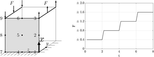
The cube is fixed on its bottom surface, where no displacements are permitted. For the other nodes, displacement is allowed only in vertical direction. A force acts on the top surface in the positive x - direction for the nodes where z = 0, and in the negative direction for the nodes where z = 1, according to the schematic in Figure 1. Over the simulation time, the force is increased four times in a stepwise manner. In this example, the cube is strongly restricted in its degrees of freedom in order to be able to clearly interpret the effects of the parameter variations and to reduce the superposition of different factors.

Figure 1. Unit cube clamped at its bottom surface, allowing for displacements at all other nodes only in the x-direction, and the corresponding external load F over time.

3.1.1. Variation of the length scale parameter

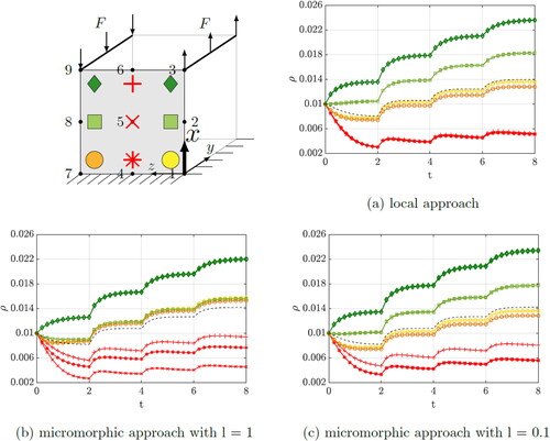
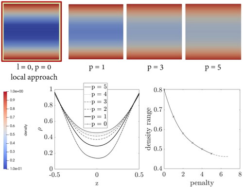
To investigate the influence of the length scale parameter l, the penalty parameter is set to p = 1 during this investigation. Since both, the boundary conditions and the forces on the cube are constant in y-direction, it is sufficient to focus on one x-z-plane. As quadratic element expansions are used, one surface of the cube consists of nine nodes, see Figure 1. The evolution of the nominal density is shown in Figure 2 for the quadrature points, which are identified with different markers. For the description of the density evolution curves we refer to quadrature points (QP 1-9) and for the displacements to the nodes (Node 1-9). The density at QP 3 and QP 9 as well as the density of QP 2 and QP 8 develop almost identically, which is why they are each marked with the same color and marker. Only close to the supports, at QP 1 and QP 7, is a difference in density due to the different loading directions visible. The density increase due to tension, at QP 1, is higher than the density increase due to compression, at QP 7. The density increase is highest at the quadrature points close to the force application and decreases in the direction of the supports. The black dashed line represents the averaged density evolution of the unit cube. The length scale parameter l can be considered as the characteristic measure of the underlying heterogeneous bone microstructure. Consequently, it can be calibrated to the size of the trabecular structure of the bone under investigation. With dimishing length scale value, the micromorphic solution converges towards the local case, see Figure 2a–c. For the local case, it can be clearly seen that the points in the unloaded part of the cube, QP 4, QP 5 and QP 6, lose density in almost the same way, i.e. the curves lie on top of each other. This changes within the micromorphic approach, where the red curves drift apart from each other according to the size of the length scale parameter.

Figure 2. Evolution of the density within the unit cube by performing the variation of the length scale parameter.

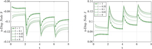
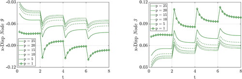
The corresponding displacements of Node 3 and Node 9 are depicted in Figure 3. As expected, the deformation of the cube increases as the length scale parameter is decreased, since the local case is approached with l = 0. It should also be mentioned that the displacement due to tension, at Node 3, is higher than the displacement due to compression, at Node 9. The fact that the density at QP 1 develops more strongly than at QP 7 also fits to this observation.

Figure 3. Evolution of the displacement of Node 3 and Node 9 of the unit cube by performing the variation of the length scale parameter.

3.1.2. Variation of the penalty parameter

Figure 4a–c show the evolution of the density with variation of the penalty parameter. The length scale parameter is set to l = 1 during this investigation.

Figure 4. Evolution of the density within the unit cube by performing the variation of the penalty parameter.

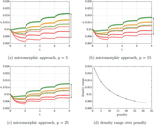
As the penalty parameter is increased, the range of the density curves is significantly affected. The higher the penalty, the more the density curves converge. Figure 4d shows the range of the density values over the penalty parameter. Above a certain penalty value, the convergence of the system can no longer be achieved because a numerical limit is reached. This is drawn as a dashed line which approaches a minimum.

The corresponding displacements of Node 3 and Node 9 are shown in Figure 5. As the penalty parameter increases, the deformation of the cube decreases significantly, which means that the cube gains stiffness, similar to the observation by Hirschberger (2008). It can be clearly seen that the displacement is approaching a minimum value with p = 25.

Figure 5. Evolution of the displacement of Node 3 and Node 9 of the unit cube by performing the variation of the penalty parameter.

3.1.3. Local vs. micromorphic approach

Finally, the classical local approach is compared to the micromorphic approach with a mixed set of length scale parameter l = 0.01 and a penalty parameter p = 25, see Figure 6.

Figure 6. Comparison of the approaches.

The length scale parameter should tend to take small values to represent a fine microstructure of the material. Whereas a large penalty parameter is used to force the macro- and microscale deformation gradients to converge. Since an opposing behaviour is to be expected, the parameters were considered individually in detail beforehand. As can be seen, the density distribution of the points differs significantly between the approaches, especially for the red points in the unloaded part of the cube. As an example, we consider QP 6, whose neighbors, QP 3 and QP 9, move in opposite directions. However, in the local approach, this point does not experience any density increase. This changes in the micromorphic approach, where the point is now also affected by the high stress of its neighbors, even though it is not directly loaded. As a result, this point experiences an increasing density. For the micromorphic approach, interaction between continuum points is evident. Thus, areas of the material that are not directly loaded also respond more to the loading of their neighbors than for the local case. The parameters control how strong the interaction is. This manifests itself in a more homogeneous density distribution and thus influences the stiffness of the body. After basic investigations have been carried out on a unit cube, a more complex example is considered in the following and the emerged findings will be discussed.

3.2. Bending of a cantilever bone specimen

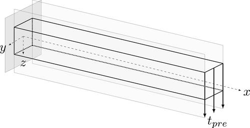
A femoral head is loaded in vertical direction by the load transferred from the hip to the hip joint. Although the actual force on a femoral head changes significantly in direction and magnitude as a function of body locomotion, the perpendicular force, represents the major component. This vertical force component causes the bone to undergo bending. In this process, the outer side of the bone (lateral cortex) experiences a tensile load, while the inner side (medial cortex) is compressed. In this example, the bending situation is investigated using a simple cantilever beam, which serves as a bone specimen from the femoral shaft region.

As shown in Figure 7, the simple cantilever beam is subjected to bending uniformly along the end face due to the applied traction t_pre.

Figure 7. Cantilever beam under bending load serving as a simplified model for the femoral shaft region.

Table 3 provides the parameters used in the model. The Young’s modulus can vary depending on the type of bone, age, etc. However, the chosen parameters are commonly used for proximal femur for the sake of demonstration, see also Carter and Beauprè (2000), Kuhl et al. (2003), Schmidt et al. (2021a) and Schaller et al. (2022). The value for the attractor stimulus, which acts as a driver for the remodelling process, and a constant traction are chosen such that the characteristics of the model are clearly visible and quantifiable. For this reason, the deformation of the beam is also larger than a real bone specimen would allow. However, for the final numerical example of the 3D femoral head, we use a lower traction that results in smaller and more realistic deformations.

Table 3. Non-dimensionalised reference parameters for the cantilever beam.

Young’s modulus	$\hspace{1em}E$	500
Poisson’s ratio	$\hspace{1em}\nu$	0.2
Initial density	$\hspace{1em}{\rho }_0^{*}$	0.4
Attractor stimulus	$\hspace{1em}{\Psi }_0^a$	0.1
Traction	$\hspace{1em}{t}_{\mathit{\text{pre}}}$	1

As for the unit cube, the variation of the length scale parameter (const. p = 1) and the variation of the penalty parameter (const. l = 1) are also performed for the bone specimen in the following.

3.2.1. Variation of the length scale parameter

The 3D beam in Figure 8 shows how the density inside the bone specimen evolved after certain time of load application given in Table 3 using the classical local approach, i.e. the length scale parameter and the penalty parameter are set to zero in this case.

Figure 8. Density distribution inside a bone specimen under bending load by performing the variation of the length scale parameter.

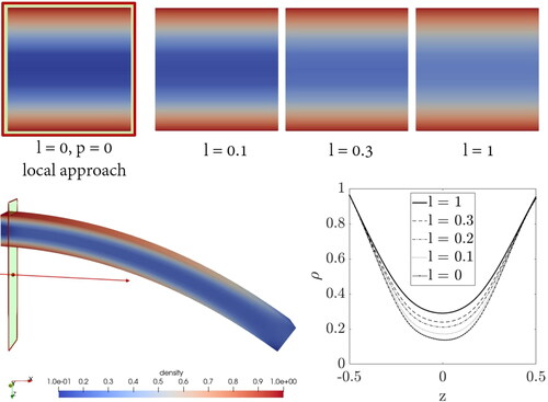
It can be seen that for the local approach the density increases mainly at the top and bottom of the beam close to the clamping, the neutral fibre of the beam does not experience any density gain. The density in this area even falls below the initial value given in Table 3. This simplified model of a bended beam from the femoral shaft region illustrates clearly why nature has evolved a hard bone cortex and a spongy bone interior in long bones due to basic loading conditions.

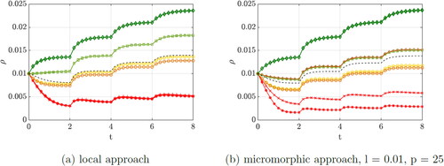
In the following, a cut-through surface of the beam next to the support is used to evaluate the differences between the approaches. The evaluation does not take place directly at the clamping in order to avoid influences of the boundary conditions. With increasing the length scale parameter, the density in the centre of the beam is increased. This means that the continuum points in the region of the neutral fibre are no longer unaffected by the loading conditions. To make this quantifiable, the diagram in Figure 8 shows the density distribution within the cross-section plotted against the z-coordinate. The centre of the beam is located at z = 0. The top and bottom area is hardly affected by the variation of the length scale. Comparing the local and the micromorphic approach, it becomes obvious that the latter is a non-local method. The interaction between the continuum points is affected in such a way that now also the points in the centre of the beam experience a density gain, depending on the value of the length scale.

3.2.2. Variation of the penalty parameter

Correspondingly, now the variation of the penalty parameter is carried out. Figure 9 shows the density distributions of the cut-through surfaces for different penalty values. The diagram shows the density distribution inside the beam in the same manner as in Figure 8. Furthermore, in the additional diagram the range of density is plotted against the corresponding penalty value. The range means that the lowest density value in the middle of the beam is subtracted from the highest value at the edge of the beam. This representation shows again a very similar behaviour to that already observed with the unit cube. The range of density values decreases with increasing penalty.

Figure 9. Density distribution inside a bone specimen under bending load by performing the variation of the penalty parameter.

The variations of the length scale parameter and the penalty parameter were performed separately. Different combinations of these parameters are discussed in the following using the final numerical example of the proximal femur.

3.3. Proximal femur

The formulation is now applied to the problem of a proximal femur. A 3D scan of a commercially available anatomical model of a femoral bone was created, surface optimised, and meshed using the tools meshmixer (Autodesk 2022) and coreform cubit (Coreform 2022).

Table 4 shows the parameters used in the model. Consequently, the same material parameters were used as for the bone specimen, except for the attractor stimulus, which was adopted as it is typically used to simulate the geometry of a whole femoral head, see also Schmidt et al. (2021a,2021b) and Schaller et al. (2022). A vertically prescribed traction of t_pre = 0.8 is applied to the femoral head to achieve a much smaller and more realistic deformation than it was the case for the beam example. The applied traction results in a displacement in the x-direction corresponding to 1.5% of the total length of the 3D femoral model shown in Figure 10.

Figure 10. Density distribution inside a femoral head using the classical local approach.

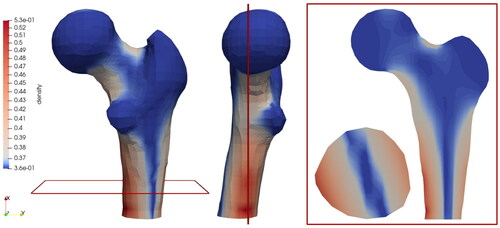
Table 4. Non-dimensionalised reference parameters for the 3D proximal femur.

Young’s modulus	$\hspace{1em}E$	500
Poisson’s ratio	$\hspace{1em}\nu$	0.2
Initial density	$\hspace{1em}{\rho }_0^{*}$	0.4
Attractor stimulus	$\hspace{1em}{\Psi }_0^a$	0.01
Traction	$\hspace{1em}{t}_{\mathit{\text{pre}}}$	0.8

Figure 10 shows the 3D model of the proximal femur using the classical local approach. Without introducing an a priori distinction between cortical and cancellous material, our model is able to predict a pronounced density increase in areas where nature also develops dense, cortical bone. Although only a simplified vertical loading condition is assumed, the areas of predicted density increase agree very well with real radiographs, e.g. from Parkinson and Fazzalari (2013) and Jacobs et al. (1995). Increased density growth can be observed mainly in the medial and lateral femoral shaft and in the neck region. It must also be acknowledged that the simplified vertical loading on the femoral head leads to an increase in density only in the medial and lateral regions, but not in the anterior and posterior regions. Since in reality the femur is also subjected to anterior and posterior loads, e.g. during running, this prescribed loading is not sufficient to fully predict the density distribution in all directions. In addition, the density distribution in the horizontal section of the femoral shaft, which is not exactly vertically aligned, is due to the fact that the bone is fixed only at the lower end. This allows rotational deformation in z-direction, i.e. not straight bending as in the previous example. Figure 10 also shows the sectional planes chosen for the detailed study in Figure 11.

Figure 11. Density distribution inside a femoral head by performing the variation of the length scale and penalty parameter.

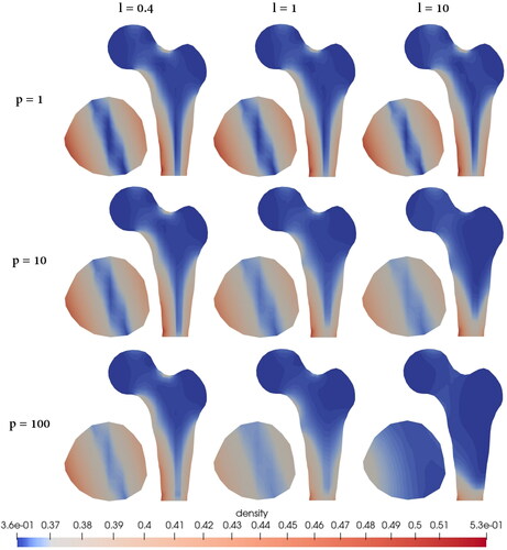
Figure 11 shows a variety of combinations where different length scale and penalty parameters were tested. In the case of a constant length scale of l = 0.1, there is hardly any difference in the variation of the penalty parameter visible. Here, the microscale contribution is so small, and thus so similar to the classical local approach, that even increasing the coupling does not make the density distribution within the bone more homogeneous, as described in the previous sections. However, when the length scale parameter, and thus the size of the microcontinuum, is increased, e.g. l = 0.4, this effect can be observed. More precisely, the larger the length scale parameter, the more pronounced this effect becomes. Furthermore, in the case of a constant penalty of p = 1, a difference in the variation of the length scale parameter is apparent but relatively small. Here, the scale bridging between micro- and macroscale deformation is minimal. With increasing the penalty, the micro- and macroscale deformations are forced to become more and more alike, resulting in a reduction of the dispersion of the density. In summary, a large penalty combined with a large length scale would result in the most homogeneous density distribution and can be interpreted as gradient elasticity.

4. Discussion and conclusion

In this work, a novel micromorphic approach for non-local bone remodelling has been proposed. Therein, a local approach for continuum bone remodelling, see, e.g. Kuhl et al. (2003), has been extended, based on Hirschberger (2008), to a micromorphic formulation and implemented into the finite element library deal.II (Bangerth et al. 2007; Arndt et al. 2022). The macroscale energy density, driving the density growth at the (quadrature) point level, is enhanced by a micromorphic energy contribution in terms of the microscale deformation gradient and a scale transition part. A penalty parameter is used to influence the coupling between micro- and macroscale deformation and a length scale parameter captures the size of the microcontinuum. The influence of these parameters has been investigated and a comparison with the classical local approach performed.

As observed by Hirschberger (2008) for the purely mechanical case, an increase of the micromorphic parameters leads to a stiffer material behaviour. As a result, the micromorphic contributions have a decisive influence on the distribution of the nominal bone density within a bone sample. To illustrate the properties of the micromorphic model, a unit cube and a cantilever beam were first studied as benchmark problems. Then, a 3D femoral head was considered as a more realistic and relevant problem. The novel micromorphic approach captures the non-local interaction between macroscale continuum points. The size of the microcontinuum and the coupling between micro- and macroscale deformation can be used to control how strong the interaction is. This is similar to Kuhl and Steinmann (2003), where the size effect was alternatively modelled by incorporation of the mass flux. There, a diffuse and almost homogeneous density distribution was observed with decreasing bone size, which corresponds to an increasing length scale in our case. In summary, it can be concluded that the consideration of non-locality has a significant impact on the density distribution in bone samples. In the proposed formulation, the non-locality of bone remodelling can be realized without an integral approach, such as presented by Mullender et al. (1994) or Schaller et al. (2022). The advantage of the micromorphic approach is that the time-consuming sampling of the mechanical stimulus in the vicinity of each point can be omitted. In addition, the early approach of Mullender et al. (1994) requires two different meshes for mechanosensing and the bone remodelling problem. Furthermore, the micromorphic approach eliminates the need for a costly two-scale model that explicitly resolves the microstructure, as presented, e.g. by Coelho et al. (2009). The metabolic cost parameter introduced there is similar in spirit of our internal length, since both can be used to influence the intensity of the density evolution. The lower the metabolic cost parameter, the more densely the bone structure develops. In our approach, we can achieve similar behaviour by increasing the internal length or penalty parameter, respectively, but without explicitly resolving the trabecular microstructure.

For future applications, the micromorphic parameters need to be chosen depending on the size and trabecular microstructure of the bone. As noted by Gitman (2012), who followed an alternative gradient elasticity approach for modelling bone tissue, determining the appropriate value for the internal length scale is a question in itself and requires a separate study. This is similar to the state of affairs in gradient plasticity, where extensive research has been conducted to establish a physical basis for the length scale. These efforts need to be applied to modelling bone adaption as well.

It is expected that with more realistic loading conditions, the characteristics of bone density growth can be captured even better. Although the rather simplified loading assumption in this work provides already very good agreement with radiographs in the coronal plane, in the future we need to represent the loading situation in the anterior and posterior directions more precisely to achieve full agreement with 3D scans of femoral heads. To this end, we will have to equip our model with improved loading scenarios, requiring an extensive load determination. Moreover, we plan integrating loading cycles from patient data into our model. Finally, muscle forces, such as the force exerted by the muscles on the greater trochanter, will also be considered as these influence the density distribution in real bone samples.

Supporting information

We provide the published figures as well as the scan of a OTC anatomical model of a femoral head via ZENODO: https://doi.org/10.5281/zenodo.7763078.

Disclosure statement

No potential conflict of interest was reported by the authors.

Additional information

Funding

This research gratefully was supported by the Deutsche Forschungsgemeinschaft (DFG, German Research Foundation) - 377472739/GRK 2434/1-2019 and the UK Engineering and Physical Sciences Research Council grant EP/R008531/1. Furthermore, we thank the Bavarian Academic Forum (BayWISS) - Doctoral Consortium ‘Health Research’ for their support.

Appendix

As indicated in Section 2.4, the remaining tangent entries are given by (22) $$\begin{array}{cc}{\partial }_{{\rho }_0}\mathbf{P}\hfill & =\frac{1}{{\rho }_0}n\mathbf{P}\hfill \\ {\partial }_{\mathbf{F}}{\mathcal{R}}_0\hfill & ={\left[\frac{{\rho }_0}{{\rho }_0^{\star }}\right]}^{-m}\mathbf{P}\hfill \\ {\partial }_{{\rho }_0}{\mathcal{R}}_0\hfill & =\left[n-m\right]{\left[\frac{{\rho }_0}{{\rho }_0^{\star }}\right]}^{-m}\frac{1}{{\rho }_0}{\Psi }_0\hfill \end{array}$$(22)

References

- Arndt D, Bangerth W, Feder M, Fehling M, Gassmöller R, Heister T, Heltai L, Kronbichler M, Maier M, Munch P, et al. 2022. The deal.ii library, version 9.4. J Numer Math. 30(3):231–246. doi:10.1515/jnma-2022-0054.
- Bagge M. 2000. A model of bone adaptation as an optimization process. J Biomech. 33(11):1349–1357. doi:10.1016/s0021-9290(00)00124-x.
- Bangerth W, Hartmann R, Kanschat G. 2007. Deal.ii—a general-purpose object-oriented finite element library. ACM Trans Math Softw. 33(4):24–es. doi:10.1145/1268776.1268779.
- Bangerth W, Heister T, Kanschat G, Maier M. 2022. The deal.ii finite element library. [accessed 2022 Sept 16]. Available from: https://www.dealii.org/.
- Carter DR, Beauprè GS. 2000. Skeletal function and form: mechanobiology of skeletal development, aging, and regeneration. Cambridge University Press. doi:10.1017/CBO9780511574993.
- Carter DR, Hayes WC. 1977. The compressive behavior of bone as a two-phase porous structure. J Bone Joint Surg Am. 59(7):954–962.
- Coelho P, Fernandes P, Rodrigues H, Cardoso J, Guedes J. 2009. Numerical modeling of bone tissue adaptation - a hierarchical approach for bone apparent density and trabecular structure. J Biomech. 42(7):830–837. doi:10.1016/j.jbiomech.2009.01.020.
- Fernandes P, Rodrigues H, Guedes J, Coelho P. 2012. Multiscale modelling on bone mechanics – application to tissue engineering and bone quality analysis. IFAC Proc Vol. 45(2):1013–1017. doi:10.3182/20120215-3-AT-3016.00179.
- Frost HM. 1987. Bone mass and the mechanostat: a proposal. Anat Rec. 219(1):1–9. doi:10.1002/ar.1092190104.
- Galilei G. 1638. Discorsi e dimostrazioni matematiche intorno á due nuove scienze attenenti alla meccanica e i movimenti locali.
- Gibson LJ, Ashby MF. 1982. The mechanics of three-dimensional cellular materials. Proc R Soc London A Math Phys Sci. 382:43–59.
- Gitman IM. 2012. Anisotropic gradient elasticity for modelling bone tissue. Comput Mater Sci. 52(1):136–138. doi:10.1016/j.commatsci.2011.06.022.
- Haj AE, Minter S, Rawlinson S, Suswillo R, Lanyon L. 1990. Cellular responses to mechanical loading in vitro. J Bone Miner Res. 5(9):923–932. doi:10.1002/jbmr.5650050905.
- Harrigan TP, Hamilton JJ. 1993. Finite element simulation of adaptive bone remodelling: a stability criterion and a time stepping method. Int J Numer Methods Eng. 36(5):837–854. doi:10.1002/nme.1620360508.
- Harrigan TP, Hamilton JJ. 1994. Necessary and sufficient conditions for global stability and uniqueness in finite element simulations of adaptive bone remodeling. Int J Solids Struct. 31(1):97–107. doi:10.1016/0020-7683(94)90178-3.
- Hirschberger CB. 2008. A treatise on micromorphic continua. theory, homogenization, computation [doctoral thesis]. Kaiserslautern: Technische Universit Kaiserslautern. ISBN: 978-3-939432-80-7.
- Hirschberger CB, Kuhl E, Steinmann P. 2007. On deformational and configurational mechanics of micromorphic hyperelasticity - theory and computation. Comput Methods Appl Mech Eng. 196(41-44):4027–4044. doi:10.1016/j.cma.2007.02.015.
- Jacobs CE, Levenston ME, Beauprè GS, Simo JC, Carter DR. 1995. Numerical instabilities in bone remodeling simulations: the advantages of a node-based finite element approach. J Biomech. 28/(4):449–459. doi:10.1016/0021-9290(94)00087-k.
- Klein-Nulend J. 2010. Mechanosensing in bone. Clinic Rev Bone Miner Metab. 8(4):161–162. doi:10.1007/s12018-011-9085-7.
- Kuhl E. 2004. Theory and numerics of open system continuum thermodynamics - spatial and material settings [habilitation]. Technische Universität Kaiserslautern.
- Kuhl E, Menzel A, Steinmann P. 2003. Computational modeling of growth - a critical review, a classification of concepts and two new consistent approaches. Comput Mech. 32(1–2):71–88. doi:10.1007/s00466-003-0463-y.
- Kuhl E, Steinmann P. 2003. Theory and numerics of geometrically non-linear open system mechanics. Int J Numer Methods Eng. 58(11):1593–1615. doi:10.1002/nme.827.
- McBride A, Davydov D, Steinmann P. 2020. Modelling the flexoelectric effect in solids: a micromorphic approach. Comput Methods Appl Mech Eng. 371:113320. doi:10.1016/j.cma.2020.113320.
- Mullender M, Huiskes R, Weinans H. 1994. A physiological approach to the simulation of bone remodeling as a self-organizational control process. J Biomech. 27(11):1389–1394. doi:10.1016/0021-9290(94)90049-3.
- Papastavrou A, Schmidt I, Deng K, Steinmann P. 2020a. On age-dependent bone remodeling. J Biomech. 103:109701. doi:10.1016/j.jbiomech.2020.109701.
- Papastavrou A, Schmidt I, Steinmann P. 2020b. On biological availability dependent bone remodeling. Comput Methods Biomech Biomed Engin. 23(8):432–444. doi:10.1080/10255842.2020.1736050.
- Park J, Park S, Kang I, Noh G. 2022a. Biomechanical effects of bone quality and design features in dental implants in long-term bone stability. J Comput Des Eng. 9(5):1538–1548. doi:10.1093/jcde/qwac069.
- Park S, Park J, Kang I, Lee H, Noh G. 2022b. Effects of assessing the bone remodeling process in biomechanical finite element stability evaluations of dental implants. Comput Methods Prog Biomed. 221:106852.
- Parkinson IH, Fazzalari NL. 2013. Characterisation of trabecular bone structure. Berlin Heidelberg: Springer; p. 31–51.
- Schaller E, Javili A, Schmidt I, Papastavrou A, Steinmann P. 2022. A peridynamic formulation for nonlocal bone remodelling. Comput Methods Biomech Biomed Eng. 25(16):1835–1851. doi:10.1080/10255842.2022.2039641.
- Scheiner S, Pivonka P, Hellmich C. 2013. Coupling systems biology with multiscale mechanics, for computer simulations of bone remodeling. Comput Methods Appl Mech Eng. 254:181–196. doi:10.1016/j.cma.2012.10.015.
- Schmidt I. 2022. Modelling and simulation of bone adaption processes [Doctoral dissertation]. Erlangen: Friedrich-Alexander-Universität Erlangen-Nürnberg.
- Schmidt I, Albert J, Ritthaler M, Papastavrou A, Steinmann P. 2021a. Bone fracture healing within a continuum bone remodelling framework. Comput Methods Biomech Biomed Eng. 25(9):1040–1050. doi:10.1080/10255842.2021.1998465.
- Schmidt I, Papastavrou A, Steinmann P. 2021b. Concurrent consideration of cortical and cancellous bone within continuum bone remodelling. Comput Methods Biomech Biomed Eng. 24(11):1274–1285. doi:10.1080/10255842.2021.1880573.
- Coreform L. 2022. Coreform cubit. [accessed 2022 Jun 27]. Available from: https://coreform.com/products/coreform-cubit/.
- Autodesk I. 2022. Autodesk meshmixer. [accessed 2022 Jul 01]. Available from: https://meshmixer.com/.