In-silico analysis of hemodynamic indicators in idealized stented coronary arteries for varying stent indentation

Abstract

In this work, we investigate the effects of stent indentation on hemodynamic indicators in stented coronary arteries. Our aim is to assess in-silico risk factors for in-stent restenosis (ISR) and thrombosis after stent implantation. The proposed model is applied to an idealized artery with Xience V stent for four indentation percentages and three mesh refinements. We analyze the patterns of hemodynamic indicators arising from different stent indentations and propose an analysis of time-averaged WSS (TAWSS), topological shear variation index (TSVI), oscillatory shear index (OSI), and relative residence time (RRT). We observe that higher indentations display higher frequency of critically low TAWSS, high TSVI, and non-physiological OSI and RRT. Furthermore, an appropriate mesh refinement is needed for accurate representation of hemodynamics in the stent vicinity. The results suggest that disturbed hemodynamics could play a role in the correlation between high indentation and ISR.

Keywords:

• Coronary arteries
• hemodynamic indicators
• stent indentation
• in-stent restenosis

1. Introduction

Cardiovascular diseases are the most common cause of death worldwide. More specifically, 30% of global mortality is due to coronary artery disease (Townsend et al. 2016; Roth et al. 2020). Its treatment largely consists in a minimally invasive surgical procedure: a coronary stent implantation. During the stent implantation, the artery wall will be injured. This triggers an inflammatory reaction which implies a number of side-effects: endothelial damage, consequent neo-intima hyperplasia (NIH), in-stent restenosis (ISR) and long term lesions with 40% occurrence rate, accumulation of platelets and possible thrombus formation, which is fatal in 45% of the cases (Holmes et al. 2010; Farooq et al. 2011). Drug-eluting stents (DES) are coated with a layer of polymer and infused with drug, designed to mitigate such side-effects (Khan et al. 2012). However, even after the introduction of DES, the percentage of stent implantation side-effects such as ISR and thrombosis is still significant (Takayama et al. 2011; Douglas 2012; Buccheri et al. 2016; McQueen et al. 2021).

Research on stent implantation ranges from balloon pressure, to drug elution, vessel injury, optimal implantation and long term effects such as ISR (Zunino et al. 2009; Antoniadis et al. 2015; Wang et al. 2015). Complex coupled models include physical and biochemical species involved in ISR, (Yang et al. 2017; Zun et al. 2017; Manjunatha et al. 2022), a structural framework for the artery wall (Romarowski et al. 2019; Silva et al. 2020), and fluid-structure interaction (FSI) between the blood and the wall (Forti et al. 2017). Numerous studies have shown the importance of altered hemodynamics in stented arteries (LaDisa et al. 2003; Zunino et al. 2009; Hachem et al. 2023), the influence of stent designs and vessel irregularities (De Santis et al. 2013) and flow patterns before and after stent implantation (Chiastra et al. 2013). Furthermore, flow patterns and recirculation areas, in particular, greatly influence drug release in DES close to the stent struts (Calo et al. 2008; Vergara and Zunino 2008; Kolachalama et al. 2009).

Blood is approximated as a homogeneous Newtonian fluid in large arteries with physiological flow (Gijsen et al. 1999; Leuprecht and Perktold 2001). Various studies have been conducted to assess shear thinning effects and blood damage in capillaries or pathological conditions (Behr et al. 2006; Behbahani et al. 2009; Marsden et al. 2014; Haßler et al. 2019; Sasse 2020). Wall shear-stress (WSS) is often used as indicator of the well-being of the cardiovascular system (Hsiao et al. 2012; Park et al. 2016; Morbiducci et al. 2020; Zingaro et al. 2021; Kronborg and Hoffman 2023). Blood recirculation occurs near areas of low WSS making them particularly dangerous: they are more prone to platelet aggregation, and therefore thrombus formation (Rayz et al. 2010), endothelial dysfunction and induced inflammation resulting in NIH (Wentzel et al. 2001; Stone et al. 2003; Nakazawa et al. 2008; Cecchi et al. 2011; Koskinas et al. 2012; Jenei et al. 2016; Brindise et al. 2017). In particular, prior studies have shown a correlation link between WSS and ISR (He et al. 2020). Hemodynamic indicators derived from WSS are time averaged WSS (TAWSS), oscillatory shear index (OSI), and relative residence time (RRT) (Soulis et al. 2011; John et al. 2017). More recently, Morbiducci et al. have introduced a topological WSS metric to classify the contraction and expansion of WSS, i.e., the topological shear index variation (TSVI), which is of high interest in stented arteries, especially to address hemodynamic effects on the endothelial surface (Chiastra et al. 2022; Mazzi et al. 2022).

One of the biggest challenges to model hemodynamics in stented arteries is to obtain the geometry of the artery lumen after stent implantation. Stent geometries can be very complex and difficult to reproduce (Auricchio et al. 2013; Zunino et al. 2016) and the arterial wall is inhomogeneous due to, e.g., calcified or necrotic areas. The artery model can be patient-specific (Kim et al. 2010), obtained from Magnetic Resonance Imaging or CT scans (Takizawa et al. 2012; Conti et al. 2016; Colombo et al. 2020) or an idealized cylindrical surface. Stents can also be implanted into the artery wall at different levels of depth, which depends on the pressure applied during the implantation. With ”stent indentation” we refer to the impression of struts into the vessel wall after stent implantation (Cornelissen et al. 2023). To achieve a satisfactory minimum stent area, e.g., with calcification, the stent has to be expanded with high pressure which results in higher indentation. Qualitative injury scores, such as the Schwartz score (Schwartz et al. 1992) are used for estimation of ISR risk post-mortem. Low injury scores have been correlated with little NIH and healthy neo-intima growth. Different levels of indentation are associated with an injury score from 0 to 3, depending on the expected side-effects. A 0 injury score is associated with 0%–10% indentation, for 10%–25% indentation injury score is 1, 25%–50% indentation results in injury score 2 and 3 is reserved for higher indentation. If the stent is only 10% indented into the artery wall, a successful stent implantation and few side effects such as ISR are expected. High indentation percentage means that a lot of pressure was applied during stent implantation and higher inflammation and vessel injury are expected. Yet the effect of indentation on hemodynamics remains uninvestigated.

In this work, we propose a 3D model of stented coronary artery for varying stent indentations and an in-silico analysis of hemodynamic indicators. We obtain a 3D CAD model of the Xience V stent (Ding et al. 2009) scanned under electronic microscope and then computationally insert it into a cylindrical idealized artery. Blood flow is modeled with Navier–Stokes equations, solved by means of stabilized Finite Element Method (FEM) and Backward Differentiation Formula (BDF) for time discretization. We investigate how indentation can influence blood flow indicators. In particular, critical areas are detected analyzing WSS, TAWSS, TSVI, OSI, RRT and their empirical frequency. In the next section, we describe the in-silico model for hemodynamics in stented arteries. In particular, Sections 2.1 and 2.2 introduce the geometry and computational domain of an idealized coronary artery lumen with a Xience V stent for varying indentations and the choice of mesh refinements. In Section 2.3, we derive the blood flow model and the hemodynamic indicators. We show the numerical results obtained for four indentation levels and three mesh refinements in Section 3. In particular, WSS, TAWSS and their critical threshold are shown in Sections 3.1, 3.2 and 3.3. We analyze the variation of WSS topological skeleton in Section 3.4, while OSI and RRT are highlighted in Section 3.5. We discuss the results and draw conclusions in Sections 4 and 5, respectively.

2. Model and method

In Sections 2.1 and 2.2, we present the workflow to obtain the computational domain of an idealized coronary artery lumen with Xience V stent at different indentation levels. The computational model for blood flow and the derivation of hemodynamic indicators are described in Section 2.3.

2.1. Geometry of expanded Xience V stent

The complex geometry of a Xience V stent is shown in Figure 1. In particular, Figure 1(a) shows the Xience V stent mounted on a delivery balloon. Figure 1(b) and (c) show the Xience V stent under scanning electron microscope, in crimped and expanded state, respectively. The strut thickness is around 80 μm and the stent length is 10.3 mm. A CAD model of the nominal configuration (factory geometry before crimping) is obtained by CARD and consequently virtually expanded to a diameter of 3.5 mm in ABAQUS by IFAM.

Figure 1. Xience V stent.

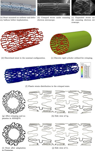
The Xience V stent geometry is discretized with 22,216 trilinear hexahedral elements with embedded incompatible modes (C3D8I) as shown in Figure 1(d). Young’s modulus of E = 222 G Pa and Poisson’s ratio of $\nu =0.29$ are used to model the elastic behavior of the cobalt-chromium (Co-Cr) alloy that constitutes the stent struts. The model is also endowed with an elastoplastic constitutive law with isotropic hardening via the prescription of the yield stress-plastic strain tuples extracted for the Co–Cr alloy from Poncin and Proft (2003). A discrete rigid cylinder (see Figure 1(e)) is used in ABAQUS to crimp the stent to the configuration shown in Figure 1(f) employing the penalty formulation for the contact between the cylinder and the stent, as well as stent self-contact. Plastic hinging is observed along the curvatures present within each cell of the strut configuration. The crimped stent is then allowed to spring back in an intermediate step. Finally, the sprung-back stent is expanded by the prescription of pressure loading on the luminal surface to obtain the configuration in Figure 1(g). The non-uniform expanded profile of the stent is attributed to the non-uniform plastic hinging induced by the crimping process. The ends of the stents are devoid of the intermediate connecting arches, thereby resulting in less plastification. This then results in the ends behaving more stiffly than the interior under pressure loading, as can be observed from Figure 1(h).

To adapt the stent geometry to an idealized cylindrical artery, we apply the following workflow using the commercial meshing software Pointwise: first, we extract the outer-most surface of the stent, then we project it onto a cylinder, and finally, we extrude the projected surface inwards to retrieve the original stent thickness of 80 μm. The final geometry is shown in Figure 1(i) and (j).

2.2. Stent indentation in lumen of idealized artery: geometry and mesh

For the artery geometry, we consider a 20 mm long segment, approximated as an ideal cylinder with a 3.6 mm diameter. The diameter is chosen based on average values of the right coronary artery (Dodge et al. 1992), and the distal length is chosen such that the artery segment completely contains the stent. This way, we can analyze the effects of stent implantation in the stent proximity, with a focus on the downstream portion.

We proceed to intersect the artery wall with the 3D model of the Xience V stent. If the stent is only lightly pushed against the artery wall, we observe a 10% indentation.High levels of indentation, e.g., 75%, imply that high pressure was applied during the surgical procedure (Cornelissen et al. 2023). Common indentation levels are between 10% and 55%, but in the scope of this work, we aim at exploring all in silico possibilities. Hence, the stent is uniformly expanded to obtain four levels of indentation: 10%, 25%, 50%, and 75%, see Figure 2(a)–(d). The artery diameter is kept at 3.6 mm and the stent is adjusted such that its external diameter is $d_S=d_A(1+\mathit{\text{In}})$ where d_A is the diameter of the lumen before the stent implantation and In is the indentation percentage. During the implantation procedure the stent is pushed further into the artery wall, therefore bending it close to the stent struts. To this extent, we define a transition area between the stent contact surface and the artery wall, highlighted in purple in Figure 2(e) and (f). The transition area is estimated based on ex-vivo microscopy imaging (Cornelissen et al. 2023). In patient-specific geometries, different indentation percentages are observed for single struts and depending on the artery configuration.

Figure 2. Geometry ((a)–(f)) and mesh ((g)–(j)) of artery lumen with Xience V stent in cross-section and longitudinal view for different indentation percentages. Figures (k)–(m) show the different mesh refinements for 75% indentation.

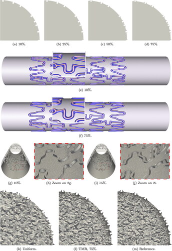
For blood flow simulations, the domain we are interested in is only the artery lumen. The lumen boundaries are obtained intersecting the inner artery wall Γ_w (cylindrical surface and transition areas) and the inner-most surface of the struts Γ_stent (see pink regions in Figure 2(e) and (f)). The external surface of the stent and the struts volume are not part of the computational domain and therefore not meshed. Figure 2(g)–(j) show the mesh resolution of the intersection surface near the transition area for two indentation levels. After meshing the intersection surface, we obtain the 3D mesh for the artery lumen. For each indentation we evaluate three mesh refinements, as shown in Figure 2(k)–(m). The uniform mesh has a mesh size of circa 0.1 mm. The reason for this is to keep the mesh elements comparable in size to the struts (Manjunatha et al. 2024). The targeted mesh refinement (TMR) case has a varying mesh size between 0.01 and 0.1 mm, where the smallest elements surround the stent and the transition areas. In the reference case, the boundary elements (artery wall, stent, and transition areas) are all kept at 0.01 mm mesh size and the volume elements transition from 0.01 to 0.1 mm mesh size from the boundary towards the center of the lumen.

2.3. Blood flow modeling and hemodynamic indicators

Incompressible Navier–Stokes equations in the Eulerian configuration describe the blood flow. The system of Equations (1)–(4)(4) $$\mathbf{u}={\mathbf{u}}_0,\text{in}\Omega \text{at}t=0,$$(4) shows the momentum and mass conservation with boundary and initial conditions: (1) $$\rho \left({\mathbf{u}}_t+\mathbf{u}·\nabla \mathbf{u}\right)-\nabla ·\mathit{\sigma }=\mathbf{0},\text{in}\Omega \times (0,T],$$(1) (2) $$\nabla ·\mathbf{u}=0,\text{in}\Omega \times (0,T],$$(2) (3) $$\mathbf{u}=\mathbf{g},\text{on}\partial \Omega ,$$(3) (4) $$\mathbf{u}={\mathbf{u}}_0,\text{in}\Omega \text{at}t=0,$$(4) where Ω is the spatial domain, $(0,T]$ denotes the time horizon, $\mathbf{u}=\mathbf{u}(\mathbf{x},t)$ is the velocity vector, $p=p(\mathbf{x},t)$ is the pressure and ρ the blood density. The stress tensor for incompressible and viscous fluids is defined as (5) $$\mathit{\sigma }=-p\mathbf{I}+2\mu \mathbf{E},$$(5) where $\mathbf{E}(\mathbf{u})=\frac{1}{2}(\nabla \mathbf{u}+\nabla {\mathbf{u}}^{\top })$ is the rate-of-strain tensor and μ is the dynamic viscosity which is assumed to be constant. Given the artery diameter of circa 3.6 mm and the idealized geometry of this work, we assume a Newtonian constitutive model for the blood (Leuprecht and Perktold 2001). 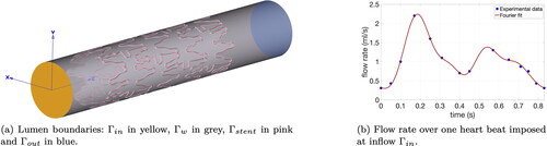Common choices for density and viscosity are ρ = 1056 kg/m³ and $\mu =3.5\times {10}^{-3}$ Pa s for 45% hematocrit and 37 °C. The artery wall is assumed to be non-moving in the presence of rigid metal stents (Moore and Berry 2002). Figure 3(a) shows the subsets of the boundary: on the artery wall Γ_w and on the stent inner surface Γ_stent, no-slip boundary conditions are imposed; on Γ_out, we impose for the velocity to be perfectly orthogonal to the outflow surface; and Γ_in has a parabolic profile. The inflow velocity magnitude is varying in time to mimic the periodic pulsatile regime over one heart beat lasting 0.83 s (Manjunatha et al. 2024). Figure 3(b) shows the Fourier interpolation of experimental data of the flow rate Q(t) in the right coronary artery (Bertolotti et al. 2001; Hsiao et al. 2012). During systole, the flow increases from a minimum flow rate of 0.31 ml/s to a maximum of 2.2 ml/s. The diastolic phase shows another increase, but the peak is much lower compared to the systolic one. Initial conditions ${\mathbf{u}}_0=\mathbf{g}(\mathbf{x},0)$ are imposed in Ω based on the velocity obtained from a steady simulation with flow rate equal to Q(0).

Figure 3. Definition of Γ and inflow boundary conditions.

We discretize system (1)(1) $$\rho \left({\mathbf{u}}_t+\mathbf{u}·\nabla \mathbf{u}\right)-\nabla ·\mathit{\sigma }=\mathbf{0},\text{in}\Omega \times (0,T],$$(1) –(4)(4) $$\mathbf{u}={\mathbf{u}}_0,\text{in}\Omega \text{at}t=0,$$(4) in space by means of stabilized FEM and we choose ${\mathbb{P}}_1-{\mathbb{P}}_1$ element pair. Given the geometry and the inflow velocity, we do not expect to be in a turbulent regime, but we expect to see vortices close to the stent struts. The maximum Reynolds number is Re = 300, thus GLS stabilization (Donea and Huerta 2003; Pauli and Behr 2017) for the momentum equation and for the incompressibility constraint is sufficient. For time discretization, we choose the BDF2 multi-step method (Forti and Dedè 2015). We linearize the convective term by means of Newton–Raphson method and solve the resulting linear system with a GMRES solver (Saad and Schultz 1986) and ILUT preconditioning (Saad 2003).

The WSS vector $\mathit{\tau }$ is computed as (John et al. 2017): (6) $$\mathit{\tau }=\mathit{\sigma }\mathbf{n}-[(\mathit{\sigma }\mathbf{n})·\mathbf{n}]\mathbf{n}=2\mu (\mathbf{\text{En}}-[(\mathbf{\text{En}})·\mathbf{n}]\mathbf{n}),$$(6) where n is the outward unit normal vector. The WSS magnitude is defined as $\text{WSS}=\left|\mathit{\tau }\right|.$ To evaluate WSS over a certain time span, a well-known quantity is TAWSS: (7) $$\text{TAWSS}=\frac{1}{T}{\int }_0^T|\mathit{\tau }(t)|\mathit{\text{dt}}.$$(7)

Taking $(0,T)$ as one heart beat cycle, TAWSS shows which areas have persistently low values of WSS. This choice is justified if the periodic flow is reached, and therefore one heartbeat is representative of any heartbeat. Averaging over multiple heartbeats would be computationally more expensive but would not add any more information.

Following Chiastra et al. (2022), we identify the divergence of the normalized WSS vector as: (8) $${\text{DIV}}_{\text{WSS}}=\nabla ·\left(\frac{\mathit{\tau }}{\left|\right|\mathit{\tau }|{|}_2}\right)=\nabla ·{\mathit{\tau }}_u,$$(8) where positive values characterize expansion and negative values correspond to contraction regions. The importance of this quantity is shown for example in Mazzi et al. (2022) and Morbiducci et al. (2020), with direct correlation to restenosis. Another related quantity of interest is TSVI, which is calculated as: (9) $$\text{TSVI}={\left\{\frac{1}{T}{\int }_0^T{\left[\nabla ·\left({\mathit{\tau }}_{\mathit{u}}\right)-\overline{\nabla ·\left({\mathit{\tau }}_{\mathit{u}}\right)}\right]}^2\mathit{\text{dt}}\right\}}^{\frac{1}{2}}.$$(9)

It quantifies the variation of WSS topological skeleton (expansion or contraction), overarching a cardiac cycle.

OSI is an indicator of the WSS deflection from the main flow direction and highlights recirculation near the artery wall: (10) $$\text{OSI}=\frac{1}{2}\left(1-\frac{|{\int }_0^T\mathit{\tau }(t)\mathit{\text{dt}}|}{{\int }_0^T|\mathit{\tau }(t)|\mathit{\text{dt}}}\right).$$(10)

It spans between 0 where shear stresses completely align with the main flow direction and 0.5 which indicates possible vortices and stagnation. RRT in (11)(11) $$\text{RRT}=\frac{1}{(1-2\text{OSI})\text{TAWSS}}.$$(11) merges the information of TAWSS and OSI in one quantity: (11) $$\text{RRT}=\frac{1}{(1-2\text{OSI})\text{TAWSS}}.$$(11)

High values of RRT correspond to low values of TAWSS and recirculation areas with high OSI values.

3. Numerical results

In this section, we analyze the numerical results obtained for the hemodynamic indicators introduced in Section 2.3 in stented arteries with a Xience V stent at different indentations. Table 1 shows an overview of mesh parameters for different refinements. The solutions obtained on the finest mesh are taken as reference. For each mesh, n_el is the total number of elements, h denotes the mesh size, and the total number of nodes is n_n. Meshes vary from 4 to 35 million elements for any indentation, depending on the refinement level. The simulation of one cycle T for a fully resolved stented artery runs for 16–17 h on 480 cores with targeted mesh refinement, while the reference case requires much more computational resources for a comparable run-time. The results are obtained after three heart beats, with time step $\Delta t=0.005$ s. The periodic regime is reached after one full heart beat. Thus, hemodynamic quantities are obtained via post-processing of the second cycle. All simulations are obtained with the highly parallelizable in-house code XNS (Pauli and Behr 2017) and are performed on the supercomputers JURECA at Forschungszentrum Jülich (Krause and Thörnig 2018) and CLAIX 2018 at RWTH Aachen University.

Table 1. Average mesh parameters for any indentation.

	nel	nn	$\overline{h}$	hmin	nn on Γ	nn on Γw	# cores	Wall-clock time
Uniform	∼ 4 M	∼ 0.7 M	0.1 mm	0.1 mm	∼ 110 K	∼ 80 K	240	∼ 3.5 h
TMR	∼ 27 M	∼ 5 M	0.1 mm	0.01 mm	∼ 1,25 M	∼ 310 K	480	∼ 16 h
Reference	∼ 35 M	∼ 6.5 M	0.1 mm	0.01 mm	∼ 2 M	∼ 900 K	960	∼ 13 h

3.1. WSS and TAWSS

We qualitatively analyze WSS and TAWSS, in particular on the reference mesh for 75% and 10% indentation.

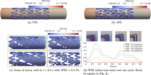
A qualitative overview of the reference WSS on the artery wall and on the stent inner surface is shown in Figure 4(a) and (b). In both cases, peaks of WSS near 1.7 Pa are observed on the stent surface, which is more exposed to the laminar flow in the lumen. In line with Manjunatha et al. (2024), the WSS values on the artery wall far away from the stent and transition areas are very similar for both indentations. We define a critical threshold for values of WSS < 0.4 Pa, which are especially problematic according to Benard et al. (2006) and Chiastra et al. (2013). Figure 4(c) highlights areas of critical WSS at time t = 0.4 s. We observe larger areas of critical WSS for 10% indentation, which decrease for higher indentations. However, if we inspect the transition areas adjacent to the stent struts as shown in Figure 4(d), the case of 75% indentation displays the lowest values of WSS over the whole cycle. On the other hand, WSS values over one cycle systematically increase for decreasing indentation percentage.

Figure 4. Reference WSS at time t  =  0.25 s for two indentation percentages (4(a) and 4(b)). Plots of critical WSS for all indentations (4(c) and 4(d)). Plots are color-coded to indentation percentages: 10% (green), 25% (blue), 50% (yellow), and 75% (red).

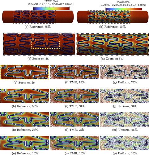
The reference TAWSS for the two extreme indentation percentages chosen in this paper is shown in Figure 5(a)–(d). We can qualitatively observe that the TAWSS values range from 0 (in blue) to 0.8 Pa (in red) and low values of TAWSS are detected in both cases close to the stent struts. However, for low indentation levels we observe a smoother transition from 0 values to physiological TAWSS. In the case of 75% indentation the transition areas are much deeper and sharper, resulting in a sudden change of TAWSS from values close to 0 to physiological ones. If we focus on a particular set of struts on the reference mesh (see Figure 5(e), (h), (k) and (n)), high indentations show larger areas of extremely low TAWSS (close to 0) and sharper transition to $\text{TAWSS}\approx 0.8$ Pa. Simulations with targeted mesh refinement (see Figure 5(f), (i), (l) and (o)) capture TAWSS values very accurately, particularly on transition areas, for all indentations. On the other hand, TAWSS values on uniform meshes (Figure 5(g), (j), (m) and (p)) roughly reproduce the indentation patterns observed for reference and targeted mesh refinement, but fail to capture the microdynamics near transition areas.

Figure 5. TAWSS for all mesh refinements and indentations.

3.2. Deviation from physiological TAWSS

To better estimate the effects of the struts and indentation compared to healthy hemodynamics, we investigate the deviation δ from the physiological TAWSS value of 0.8 Pa (Manjunatha et al. 2024), defined as: (12) $$\delta =\frac{|\text{TAWSS}-0.8|}{0.8}.$$(12)

A deviation close to 0 corresponds to values within a healthy range, while a δ close to 1 highlights critical values of TAWSS. In Figure 6(a) and (b) we observe that the transition pattern for 10% and 75% is similar to the one observed in Figure 5: the case of 75% indentation shows highly deviating values in the transition areas and 10% indentation gradually transitions from deviating values in the stent vicinity to 0 deviation on the non-deformed artery wall; see strut details in Figure 6(c) and (d).

Figure 6. Reference TAWSS deviation δ for two indentation percentages.

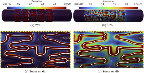
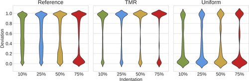
Figure 7 provides an overview of indentation percentage effects on the deviation δ for all mesh refinements. The violin plots estimate the density distribution of δ, based on the number of mesh nodes associated with a certain deviation value. In the reference case, we observe that low indentations have a more uniformly distributed deviation between 0 and 1, which becomes more hour-glass-shaped for higher indentations. In particular, 75% indentation has the highest density of both $\delta \approx 1$ and $\delta \approx 0.$ The simulations with targeted mesh refinement reproduce qualitatively accurate results for all indentation percentages, in particular for deviation $\delta \approx 1$ in the stent proximity. Physiological TAWSS values are located where the targeted refined mesh is coarser. Therefore all indentations have low density for $\delta <0.6.$ In the uniform case, the deviation trend for all indentations is similar for $\delta \approx 1.$ However, the density distribution is much larger for $\delta \approx 0,$ inverting the trend shown in the reference case.

Figure 7. Violin plots of δ density distribution for all mesh refinements and indentations.

3.3. Critical values of TAWSS

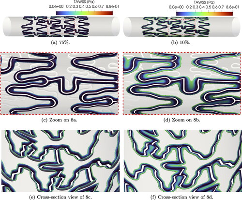
In this subsection, we analyze the critical sub-threshold TAWSS between 0 and 0.4 Pa (Benard et al. 2006; Chiastra et al. 2013) both qualitatively and quantitatively.

Figure 8 highlights where critical values are located, i.e., in the vicinity of the stent struts, almost completely overlapping with the transition areas for 75% indentation, as shown in Figure 8(e). The highlighted struts in Figure 8(c) also showcase that for high indentation we observe small TAWSS variance and high density of values close to 0. On the other hand, low values of TAWSS for 10% indentation are spread over a larger portion of artery wall and showcase higher density of TAWSS towards the upper end of the critical values range (see Figure 8(d) and (f)).

Figure 8. Areas of artery wall with TAWSS < 0.4 Pa on reference mesh for two indentation percentages.

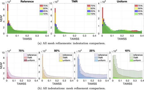
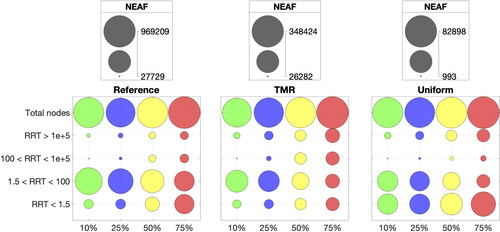
A quantitative analysis is provided by plotting the nodal absolute empirical frequency (NEAF) of TAWSS values smaller than 0.4 Pa in the form of histograms. The NEAF is calculated by counting the number of mesh nodes with TAWSS within a certain range. Figure 9(a) and (b) show the TAWSS histograms grouped by mesh refinements and indentations respectively. We choose a uniform bin width of 0.01 Pa for a total of 40 bins per histogram. For the reference mesh (see left-most subplot in Figure 9(a)), 75% indentation has the highest NEAF of TAWSS values between 0 and 0.01 Pa and the NEAF of the first bin decreases with indentation percentage. On the other hand, 10% indentation has the highest NEAF of values between 0.39 and 0.4 Pa. From Figure 9(b), we observe that for each indentation, NEAFs show a similarly decaying trend from $\text{TAWSS}=0$ to $\text{TAWSS}=0.4$ Pa in the case of targeted mesh refinement and reference mesh. This pattern is not present for the uniform meshes, where the NEAF variance is much higher between bins (see right-most subplot in Figure 9(a)).

Figure 9. NEAF histograms of TAWSS < 0.4 Pa.

To prevent errors of NEAF estimation, we refine the histogram bin width to 0.0002 Pa and plot the histogram data in Figure 10(a). Looking at the reference mesh (left-most subplot) the highest NEAF is accumulated close to zero for 75% indentation and decreases (in order) for 50%, 25% and 10% indentation. The NEAF decay is very fast for high indentations and slower for low indentations. This entails that the reference NEAF order is inverted for values close to 0.4 Pa. The highest NEAF in the upper end range is given by 10% indentation and decreases with increasing indentation, i.e., (in order) 25%, 50% and 75%. Low values of TAWSS have very close NEAF for each indentation in targeted mesh refinement and reference cases, especially for values smaller than 0.25 Pa. NEAF values with uniform meshes and targeted mesh refinement for $\text{TAWSS}>0.25$ Pa are hard to evaluate, since the refined bin size introduces a lot of noise.

Figure 10. NEAF plots of TAWSS < 0.4 Pa.

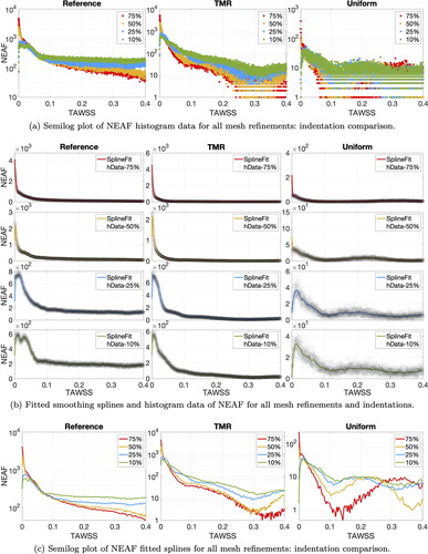
To exclude additional noise added by the small histogram bin size, we interpolate the histogram values with splines (Eilers and Marx 2010) using Matlab Curve Fitting Tool (The MathWorks 2021) for visual convenience. We ensure that the goodness of fit is satisfactory, by imposing $R^2>0.9.$ The curves obtained are compared to the raw histogram data for each indentation and mesh refinement in Figure 10(b). Figure 10(c) groups the fitted curves for each mesh refinement. Comparing targeted mesh refinement and reference case, we observe a similar decay for each indentation percentage and nearly identical NEAF for $\text{TAWSS}=0.$ Furthermore, the same NEAF decaying order is retrieved with targeted mesh refinement for values of TAWSS close to 0.4 Pa. This NEAF pattern is not reproduced with uniform meshes, in particular for high indentations (see right-most subplots in Figure 10(c)).

3.4. WSS divergence and TSVI

In this section we describe the main results observed in the WSS topological skeleton for two indentations, namely 75% and 10%.

In Figure 11, we examine the divergence of the normalized cycle-averaged WSS vector, ${\text{DIV}}_{\text{WSS}},$ focusing on expansion and contraction regions. Expansion regions, depicted in red, coincide with positive values of ${\text{DIV}}_{\text{WSS}},$ while contraction regions, in blue, correspond to negative values. For both indentation, a recurrent pattern emerges: upstream stent struts exhibit expansion, while downstream stent struts show contraction. At 75% indentation, regions of expansion and contraction are localized near the transition regions, similarly to what observed for critical TAWSS. In contrast, at 10% indentation, expansion and contraction regions appear more spread out along the stented artery wall.

Figure 11. Cycle-averaged WSS topological skeleton on reference mesh and two indentation percentages. ${\text{DIV}}_{\text{WSS}}$ is calculated in $m^{-1}.$

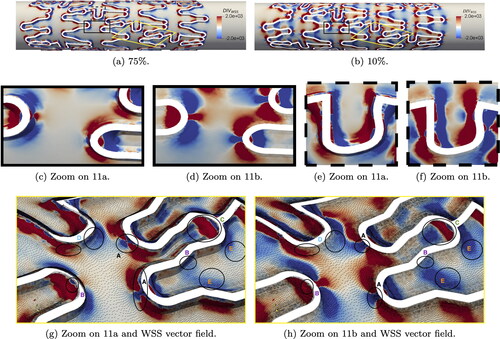
Notably, struts with tips orthogonal to the flow direction exhibit a distinct pattern (see Figure 11(c) and (d)): contraction around the strut tip is followed by expansion immediately around it, with the opposite pattern observed if the tip faces downstream direction. Furthermore, in U-shaped struts perpendicular to the flow direction, expansion-contraction patterns occur twice, as highlighted in Figure 11(e) and (f).

To facilitate comparison between the two indentations, we zoom in on some struts from a different perspective in Figure 11(g) and (h). Here, we also plot the WSS vector field, highlighting that contraction regions correspond to streamline accumulation and expansion regions correspond to divergent streamlines, as described in Chiastra et al. (2022). Additionally, within these figures, we mark areas of interest for comparison and analysis in the following paragraph. In areas marked with A, contraction is focused on the strut tip for 10% indentation, whereas at 75% indentation, contraction expands around the strut, closely following its shape. Larger and more numerous contraction areas are observed at 75% indentation (see e.g. left-most area B). Also on longitudinal struts marked as B, contraction is evident, whereas little to no contraction is observed for 10% indentation. Expansion areas, marked with C, appear larger in some cases, compared to 10% indentation. Focusing on U-shaped struts, marked as D, larger areas of contraction and expansion extend along the artery wall, aligning with the stent strut profile, for 75% indentation. Conversely, lower indentations exhibit larger areas of altered WSS topological skeleton further away from the transition areas, marked with E.

The TSVI quantifies the amount of variation in WSS expansion or contraction over the cardiac cycle. Following Chiastra et al. (2022), the values in Figure 12 were capped at 5000 $m^{-1}.$

Figure 12. TSVI in $m^{-1}$ for all mesh refinements and two indentation percentages.

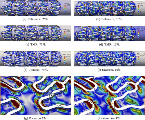
Comparing TSVI values to the reference case (Figure 12(a) and (b)), regions of high TSVI are accurately captured for both indentations when using targeted mesh refinement, as depicted in Figure 12(c) and (d). On the other hand, uniform meshes result in significant inaccuracies, as shown in Figure 12(e) and (f).

For the reference case, we highlight specific areas of interest in Figure 12(g) and (h), which we further discuss in the following paragraph. At 10% indentation, areas of higher TSVI (greater than 3000 $m^{-1}$) are observed in the stented wall, albeit distant from the transition areas (see area marked with A). Furthermore, high TSVI values are more dispersed within the stented area, tending towards values around 1000 $m^{-1}.$ Conversely, for 75% indentation, areas of high TSVI predominantly surround the transition areas (also highlighted with A), similarly to what observed for ${\text{DIV}}_{\text{WSS}}.$ Additionally, areas with TSVI exceeding 5000 $m^{-1}$ are more extensive compared to 10% indentation (see areas marked with B for both cases). Overall, regions of high TSVI tend to coincide with areas of low TAWSS. However, high TSVI values (greater than 4000 $m^{-1}$) are localized at the tips of struts, both upstream and downstream, and around struts orthogonal to the main flow direction (see zones marked as C).

3.5. OSI, RRT and limit values

Effects of indentation on OSI and RRT are analyzed in this section.

Figure 13(c) shows that 75% indentation results in increased areas with OSI = 0.5, i.e., more stagnation around the stent struts, compared to 10% indentation (see Figure 13(f)). The targeted mesh refinement is able to accurately capture the critical areas of OSI = 0.5 for both indentation percentages, as shown in Figure 13(d) and (g). The uniform meshes underestimate the OSI value in several areas around the stent (Figure 13(e) and (h)). Most values of OSI are either very close to 0 or very close to 0.5. This pattern is detected for all indentation and refinements in Figure 14. The bubble plot shows the NEAF for OSI < 0.01, 0.01 < OSI < 0.5 and OSI = 0.5. The comparison between the total number of nodes and the NEAF for OSI in different value ranges show that the majority of mesh nodes detect $\text{OSI}<0.01.$ Only a small fraction of total nodes show limit values of OSI, which we compare in more detail in Figure 15.

Figure 13. OSI for all mesh refinements and two indentation percentages.

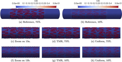
Figure 14. NEAF bubble chart of OSI for all mesh refinements and indentations.

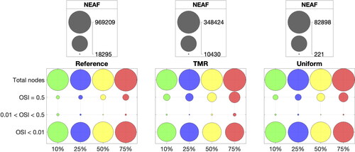
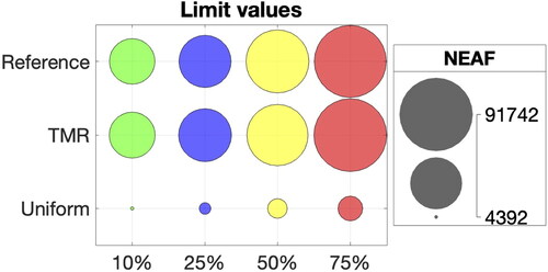
Figure 15. NEAF bubble chart of hemodynamic indicators at limit values.

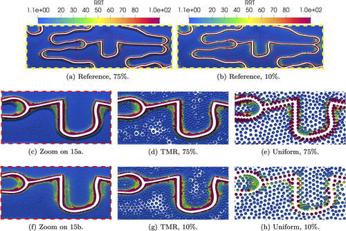
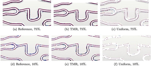
The physiological healthy RRT value is approximately 1.3 $\frac{1}{\mathit{\text{Pa}}}$ (Manjunatha et al. 2024). Higher values entail both low WSS and recirculation. For the reference cases in Figure 16(a) and (c), we observe that 75% indentation have larger areas of critically high RRT values, while 10% indentation shows a more spread-out distribution of RRT (Figure 16(b) and (f)). For both indentations, reference physiological values of RRT are observed far away from the stent. Figure 16(d) and (g) highlight how targeted mesh refinement is able to correctly capture the same RRT values very close to the stent strut and the complex microdynamics in the surrounding area. In the case of uniform meshes (Figure 16(e) and (h)) RRT values are underestimated, especially in the stent proximity.

Figure 16. RRT for all mesh refinements and two indentations. Details of yellow dashed zoombox in Figure 5(c).

Figure 17 shows the NEAF for different RRT ranges. Most RRT values are classified between 0 and 100 $\frac{1}{\mathit{\text{Pa}}}.$ Values of RRT between 1.5 and 100 $\frac{1}{\mathit{\text{Pa}}}$ represent the areas of low TAWSS between 0.1 and 0.4 Pa and mild recirculation. For each indentation, we notice that the reference NEAF of 1.5 < RRT < 100 decreases for increasing indentation percentage, and that NEAF for $\text{RRT}>$ 100 increases consistently from 10% to 75% indentation. This pattern is also observed for all indentations with targeted mesh refinement, but the uniform meshes seem to miss most of the microdynamics in the range 100 < RRT < 1e + 5 compared to the targeted mesh refinement and reference cases.

Figure 17. NEAF bubble chart of RRT for all mesh refinements and indentations.

Limit values of $\text{RRT}>$ 1e + 5 are represented by values of $\text{TAWSS}=0$ and $\text{OSI}=0.5.$ Figure 18 highlight the areas with limit values for all mesh refinements with 75% and 10% indentation. These values surround the stent profile for both indentations. Looking at the reference cases, higher indentations show larger areas of limit values compared to 10% indentation. The targeted mesh refinement reproduces very closely the limit values in the same areas of the artery wall. In the uniform case, large areas of limit values are missed, with underestimated RRT. The reference NEAF of limit values for RRT > 1e + 5 steadily increases for higher indentation percentages as shown in Figure 15 for all mesh refinements. However, NEAF values for reference and targeted mesh refinement are almost identical, while uniform meshes display much smaller NEAF for each indentation.

Figure 18. Areas of artery wall with limit values of hemodynamic indicators for all mesh refinements and two indentations. Zoom detail from Figure 16.

4. Discussion

The analysis of blood velocity streamlines in Manjunatha et al. (2024) show that small vortices are located near the stent struts. For this reason, we choose three mesh refinements with focus on the transition areas. Furthermore, hemodynamic indicators are more practical and can more precisely highlight the critical areas, compared to a qualitative analysis of streamlines.

From Cornelissen et al. (2023), we expect to see WSS values closer to physiological ones in stented arteries with low indentation. In apparent contradiction, Figure 4(c) shows that for 10% indentation we have larger areas of low WSS. This is due to the fact that low indentation means that the protruding stent shields the artery wall, which is therefore less exposed to the blood flow. However, Figure 4(d) shows that in the stent vicinity, the critical WSS magnitude increases for decreasing indentation with the following order (from lowest to highest values): 75%, 50%, 25%, and 10%. Values of WSS can temporarily exceed the physiological range, but relevant side-effects are observed when low values of WSS are persistent. Thus, we make use of time-averaged indicators to highlight the critical areas over one cycle. High indentations have sharp variations of hemodynamic indicators from limit to physiological values, while lower indentations gradually span the whole values range. Most non-physiological values are concentrated in the transition area, especially for higher indentations. Thus, targeted mesh refinement provides good accuracy thanks to the refinement in the stent vicinity.

For a more quantitative overview, we investigate the empirical frequency of hemodynamic indicators, with a focus on critical values. Plotting frequency as histograms in Figure 9, we notice that higher indentations have larger areas of sub-threshold TAWSS, i.e., higher NEAF for $\text{TAWSS}=0,$ and that the decaying order observed for WSS is maintained. Targeted mesh refinement shows very similar frequency trends for all indentations, compared to the reference case. The uniform mesh fails to maintain the frequency decaying order for TAWSS values close to 0.4 Pa.

From the analysis of ${\text{DIV}}_{\text{WSS}},$ we observe that lower indentations cause less disturbance to the WSS topological skeleton, particularly near the stent. In contrast, 75% indentation display more frequent alternations between contraction and expansion. Furthermore, critical areas are larger and TSVI values are higher for 75% indentation. In general, we find that the regions exhibiting the largest variations in the WSS topological skeleton, are typically located near struts with orthogonal curvature to the main flow direction, both upstream and downstream. This observation marks a difference compared to sub-threshold TAWSS, where all transition areas around the stent were identified as critical.

Frequency of critical OSI and RRT values also increase with indentation percentage. From Figures 15 and 18, the targeted mesh refinement is able to reproduce very closely the reference frequency for limit values and to detect the same reference areas on the artery wall. Uniform meshes seem to be too coarse to accurately track areas at critical risk of ISR and these results are confirmed when evaluating the corresponding NEAF for all indentations.

4.1. Outlook and limitations

Stent indentation occurs due to the pressure applied during stent implantation. Within allowed margins and under certain circumstances, clinicians can regulate the pressure during percutaneous coronary intervention. By simulating the stenting procedure beforehand, clinicians could optimize pressure levels to achieve better implantation outcomes, considering changes in hemodynamic indicators. Moreover, advanced techniques may involve directly linking hemodynamic indicators to in-stent restenosis (ISR), thereby predicting the scenario with the least ISR. This preliminary investigation aims to identify the most relevant indicators. It also suggests that it might be beneficial to incorporate their influence in growth models, especially for fine-tuning ISR prediction models, in line with the work of Sáez et al. (2015).

This study acknowledges several limitations in the modeling approach. The choice of an idealized cylindrical artery overlooks the complexity arising from artery curvature, bifurcations, and patient-specific variations. Assuming rigid walls neglects the arterial response to stent implantation and its elastic response to pressure and heart movement. Stents do not always adhere perfectly to the arterial wall, leading to non-uniform expansion and malapposition. Furthermore, the influence of calcification and plaque type is not considered. Transition areas in our model are artificially defined, which does not reflect the variability in indentation levels for each strut in the same stented artery. The model also considers a simple coronary artery inflow, yet incorporating Windkessel boundary conditions and elastic response of the artery wall could significantly impact hemodynamic indicators. Hence, validation efforts are necessary, requiring assessing the influence of realistic artery geometries, alternative stent designs, and complex boundary conditions to determine which indicators are more relevant for ISR prediction. Within the scope of this project we plan to fully couple the hemodynamics simulations to the moving wall in an FSI fashion to model both ISR and artery pulsation. For a clinical setting, the current computational costs are not feasible for an ISR predictive study. The authors are investigating model reduction techniques based on Zunino et al. (2016) and Brandes Costa Barbosa and Perotto (2020) to further reduce the computational effort.

5. Conclusions

In this paper we investigate the effects of stent indentation on hemodynamic indicators in coronary arteries. Our goal is to provide an in-silico study examining potential ISR risk factors due to blood flow alterations. To the best of our knowledge, there have been no numerical studies of hemodynamics in stented coronary arteries focusing on indentation effects. We investigate four indentation percentages with particular focus on sub-threshold TAWSS, high TSVI, and limit values of OSI and RRT.

We opt for an idealized cylindrical artery for conveniently calculating indentation percentages based on the initial diameter and for control on the extent of the transition area. We use the widely employed Xience V stent in all cases to emphasize the impact of indentation, while excluding other influencing factors such as stent design. These choices are made for computational convenience. However, they come with a number of limitations, due to the significantly simplified model compared to real-world scenarios, which we discuss in detail in Section 4.1.

The study on three mesh refinements shows that targeted mesh refinement can moderately reduce computational costs while preserving enough accuracy. In particular, reference and targeted mesh refinement cases show nearly identical trends of low TAWSS frequency, high TSVI, and limit values of OSI and RRT, while uniform meshes fail to detect such pattern. In particular, we observe that a mesh size only comparable to the stent diameter is not sufficient. However, mesh elements with diameter one order of magnitude smaller than the stent characteristic size, albeit limited to the transition volume, seem to be sufficiently accurate for the specific case of idealized artery and indentation.

Non-physiological values of hemodynamic indicators are detected close to the stent struts, mostly in the transition areas. Higher indentation percentages have higher frequency of sub-threshold TAWSS, higher TSVI, as well as critical OSI and RRT. In Cornelissen et al. (2023), higher indentation correlates with higher risk of ISR. Thus, altered hemodynamics could play a role in this relationship. Hence, it may be worth taking indentation into account in predictive studies of stent implantation outcomes, especially in clinical contexts. This is particularly pertinent when hemodynamic indicators are among the predictive parameters. Additionally, this study could serve as an initial step towards investigating the impact of hemodynamic indicators on ISR growth models.

Acknowledgements

The authors especially thank Jana Sasse for her work on blood model investigations, Svenja Nerzak for her numerous contributions to the geometry, mesh modeling and model testing, Henrik Volgmann for his work during his project thesis and Michael Aichmüller for fruitful discussions. We especially thank Ulrich Fuchs for his guidance in mesh generation with Pointwise.

The authors gratefully acknowledge the computing time granted through JARA-HPC on the supercomputer JURECA at Forschungszentrum Jülich and on the supercomputer CLAIX at RWTH Aachen University. The authors gratefully acknowledge the computing time provided to them on the high-performance computer Lichtenberg at the NHR Centers NHR4CES at TU Darmstadt. This is funded by the Federal Ministry of Education and Research, and the state governments participating on the basis of the resolutions of the GWK for national high performance computing at universities (www.nhr-verein.de/unsere-partner).

Disclosure statement

No potential conflict of interest was reported by the authors.

Additional information

Funding

This work has been funded through the financial support of German Research Foundation (DFG) for the project “Drug-eluting coronary stents in stenosed arteries: medical investigation and computational modelling” (project number 395712048:BE 3689/15, RE 1057/44, VO1624/5) and for the subproject “In-stent restenosis in coronary arteries – in silico investigations based on patient-specific data and meta modeling” of SPP2311. This work was also partly supported by the IRTG-2379 Modern Inverse Problems which is funded by the DFG-333849990/GRK2379.

References

- Antoniadis AP, Mortier P, Kassab G, Dubini G, Foin N, Murasato Y, Giannopoulos AA, Tu S, Iwasaki K, Hikichi Y, et al. 2015. Biomechanical modeling to improve coronary artery bifurcation stenting: expert review document on techniques and clinical implementation. JACC Cardiovasc Interv. 8(10):1281–1296. doi: 10.1016/j.jcin.2015.06.015.
- Auricchio F, Conti M, Ferrara A, Morganti S, Reali A. 2013. Patient-specific finite element analysis of carotid artery stenting: a focus on vessel modeling. Int J Numer Method Biomed Eng. 29(6):645–664. doi: 10.1002/cnm.2511.
- Behbahani M, Behr M, Hormes M, Steinseifer U, Arora D, Coronado O, Pasquali M. 2009. A review of computational fluid dynamics analysis of blood pumps. Eur J Appl Math. 20(4):363–397. doi: 10.1017/S0956792509007839.
- Behr M, Arora D, Coronado O, Pasquali M. 2006. Models and finite element techniques for blood flow simulation. Int J Computat Fluid Dyn. 20(3-4):175–181. doi: 10.1080/10618560600789776.
- Benard N, Perrault R, Coisne D. 2006. Computational approach to estimating the effects of blood properties on changes in intra-stent flow. Ann Biomed Eng. 34(8):1259–1271. doi: 10.1007/s10439-006-9123-7.
- Bertolotti C, Deplano V, Fuseri J, Dupouy P. 2001. Numerical and experimental models of post-operative realistic flows in stenosed coronary bypasses. J Biomech. 34(8):1049–1064. doi: 10.1016/s0021-9290(01)00027-6.
- Brandes Costa Barbosa YA, Perotto S. 2020. Hierarchically reduced models for the stokes problem in patient-specific artery segments. Int J Computat Fluid Dyn. 34(2):160–171. doi: 10.1080/10618562.2020.1733537.
- Brindise MC, Chiastra C, Burzotta F, Migliavacca F, Vlachos PP. 2017. Hemodynamics of stent implantation procedures in coronary bifurcations: an in vitro study. Ann Biomed Eng. 45(3):542–553. doi: 10.1007/s10439-016-1699-y.
- Buccheri D, Piraino D, Andolina G, Cortese B. 2016. Understanding and managing in-stent restenosis: a review of clinical data, from pathogenesis to treatment. J Thorac Dis. 8(10):E1150–E1162. doi: 10.21037/jtd.2016.10.93.
- Calo V, Brasher N, Bazilevs Y, Hughes T. 2008. Multiphysics model for blood flow and drug transport with application to patient-specific coronary artery flow. Comput Mech. 43(1):161–177. doi: 10.1007/s00466-008-0321-z.
- Cecchi E, Giglioli C, Valente S, Lazzeri C, Gensini GF, Abbate R, Mannini L. 2011. Role of hemodynamic shear stress in cardiovascular disease. Atherosclerosis. 214(2):249–256. doi: 10.1016/j.atherosclerosis.2010.09.008.
- Chiastra C, Mazzi V, Lodi Rizzini M, Calò K, Corti A, Acquasanta A, De Nisco G, Belliggiano D, Cerrato E, Gallo D, et al. 2022. Coronary artery stenting affects wall shear stress topological skeleton. J Biomech Eng. 144(6):061002. doi: 10.1115/1.4053503.
- Chiastra C, Morlacchi S, Gallo D, Morbiducci U, Cárdenes R, Larrabide I, Migliavacca F. 2013. Computational fluid dynamic simulations of image-based stented coronary bifurcation models. J R Soc Interface. 10(84):20130193. doi: 10.1098/rsif.2013.0193.
- Colombo M, Bologna M, Garbey M, Berceli S, He Y, Matas JFR, Migliavacca F, Chiastra C. 2020. Computing patient-specific hemodynamics in stented femoral artery models obtained from computed tomography using a validated 3D reconstruction method. Med Eng Phys. 75:23–35. doi: 10.1016/j.medengphy.2019.10.005.
- Conti M, Long C, Marconi M, Berchiolli R, Bazilevs Y, Reali A. 2016. Carotid artery hemodynamics before and after stenting: a patient specific CFD study. Comput Fluids. 141:62–74. doi: 10.1016/j.compfluid.2016.04.006.
- Cornelissen A, Florescu RA, Reese S, Behr M, Ranno A, Manjunatha K, Schaaps N, Böhm C, Liehn EA, Zhao L, et al. 2023. In-vivo assessment of vascular injury for the prediction of in-stent restenosis. Int J Cardiol. 388:131151. doi: 10.1016/j.ijcard.2023.131151.
- De Santis G, Trachet B, Conti M, De Beule M, Morbiducci U, Mortier P, Segers P, Verdonck P, Verhegghe B. 2013. A computational study of the hemodynamic impact of open-versus closed-cell stent design in carotid artery stenting. Artif Organs. 37(7):E96–106. doi: 10.1111/aor.12046.
- Ding N, Pacetti SD, Tang FW, Gada M, Roorda W. 2009. Xience V™ stent design and rationale. J Interven Cardiol. 22(s1):S18–S27. doi: 10.1111/j.1540-8183.2009.00450.x.
- Dodge JT, Brown BG, Bolson EL, Dodge HT. 1992. Lumen diameter of normal human coronary arteries. influence of age, sex, anatomic variation, and left ventricular hypertrophy or dilation. Circulation. 86(1):232–246. doi: 10.1161/01.cir.86.1.232.
- Donea J, Huerta A. 2003. Finite element methods for flow problems. Chichester, England: John Wiley & Sons.
- Douglas JS. 2012. Drug-eluting stent restenosis: a need for new technology? JACC Cardiovasc Interv. 5(7):738–740. doi: 10.1016/j.jcin.2012.03.019.
- Eilers PH, Marx BD. 2010. Splines, knots, and penalties. WIREs Computat Stats. 2(6):637–653. doi: 10.1002/wics.125.
- Farooq V, Gogas BD, Serruys PW. 2011. Restenosis: delineating the numerous causes of drug-eluting stent restenosis. Circ Cardiovasc Interv. 4(2):195–205. doi: 10.1161/CIRCINTERVENTIONS.110.959882.
- Forti D, Bukac M, Quaini A, Canic S, Deparis S. 2017. A monolithic approach to fluid–composite structure interaction. J Sci Comput. 72(1):396–421. doi: 10.1007/s10915-017-0363-5.
- Forti D, Dedè L. 2015. Semi-implicit BDF time discretization of the Navier–Stokes equations with VMS-les modeling in a high performance computing framework. Comput Fluids. 117:168–182. doi: 10.1016/j.compfluid.2015.05.011.
- Gijsen FJ, van de Vosse FN, Janssen J. 1999. The influence of the non-Newtonian properties of blood on the flow in large arteries: steady flow in a carotid bifurcation model. J Biomech. 32(6):601–608. doi: 10.1016/s0021-9290(99)00015-9.
- Hachem E, Meliga P, Goetz A, Rico PJ, Viquerat J, Larcher A, Valette R, Sanches A, Lannelongue V, Ghraieb H, et al. 2023. Reinforcement learning for patient-specific optimal stenting of intracranial aneurysms. Sci Rep. 13(1):7147. doi: 10.1038/s41598-023-34007-z.
- Haßler S, Pauli L, Behr M. 2019. The variational multiscale formulation for the fully-implicit log-morphology equation as a tensor-based blood damage model. Int J Numer Method Biomed Eng. 35(12):e3262. doi: 10.1002/cnm.3262.
- He R, Zhao L, Silberschmidt VV, Liu Y. 2020. Mechanistic evaluation of long-term in-stent restenosis based on models of tissue damage and growth. Biomech Model Mechanobiol. 19(5):1425–1446. doi: 10.1007/s10237-019-01279-2.
- Holmes DR, Kereiakes DJ, Garg S, Serruys PW, Dehmer GJ, Ellis SG, Williams DO, Kimura T, Moliterno DJ. 2010. Stent thrombosis. J Am Coll Cardiol. 56(17):1357–1365. doi: 10.1016/j.jacc.2010.07.016.
- Hsiao HM, Lee KH, Liao YC, Cheng YC. 2012. Hemodynamic simulation of intra-stent blood flow. Procedia Eng. 36:128–136. doi: 10.1016/j.proeng.2012.03.020.
- Jenei C, Balogh E, Szabó GT, Dézsi CA, Kőszegi Z. 2016. Wall shear stress in the development of in-stent restenosis revisited. a critical review of clinical data on shear stress after intracoronary stent implantation. Cardiol J. 23(4):365–373. doi: 10.5603/CJ.a2016.0047.
- John L, Pustějovská P, Steinbach O. 2017. On the influence of the wall shear stress vector form on hemodynamic indicators. Comput Visual Sci. 18(4-5):113–122. doi: 10.1007/s00791-017-0277-7.
- Khan W, Farah S, Domb AJ. 2012. Drug eluting stents: developments and current status. J Control Release. 161(2):703–712. doi: 10.1016/j.jconrel.2012.02.010.
- Kim HJ, Vignon-Clementel I, Coogan J, Figueroa C, Jansen K, Taylor C. 2010. Patient-specific modeling of blood flow and pressure in human coronary arteries. Ann Biomed Eng. 38(10):3195–3209. doi: 10.1007/s10439-010-0083-6.
- Kolachalama VB, Tzafriri AR, Arifin DY, Edelman ER. 2009. Luminal flow patterns dictate arterial drug deposition in stent-based delivery. J Control Release. 133(1):24–30. doi: 10.1016/j.jconrel.2008.09.075.
- Koskinas KC, Chatzizisis YS, Antoniadis AP, Giannoglou GD. 2012. Role of endothelial shear stress in stent restenosis and thrombosis: pathophysiologic mechanisms and implications for clinical translation. J Am Coll Cardiol. 59(15):1337–1349. doi: 10.1016/j.jacc.2011.10.903.
- Krause D, Thörnig P. 2018. Jureca: modular supercomputer at jülich supercomputing centre. JLSRF. 4: a 132. doi: 10.17815/jlsrf-4-121-1.
- Kronborg J, Hoffman J. 2023. The triple decomposition of the velocity gradient tensor as a standardized real schur form. Phys Fluids. 35(3):031703. doi: 10.1063/5.0138180.
- LaDisa JF, Guler I, Olson LE, Hettrick DA, Kersten JR, Warltier DC, Pagel PS. 2003. Three-dimensional computational fluid dynamics modeling of alterations in coronary wall shear stress produced by stent implantation. Ann Biomed Eng. 31(8):972–980. doi: 10.1114/1.1588654.
- Leuprecht A, Perktold K. 2001. Computer simulation of non-newtonian effects on blood flow in large arteries. Comput Methods Biomech Biomed Engin. 4(2):149–163. doi: 10.1080/10255840008908002.
- Manjunatha K, Behr M, Vogt F, Reese S. 2022. A multiphysics modeling approach for in-stent restenosis: theoretical aspects and finite element implementation. Comput Biol Med. 150:106166. doi: 10.1016/j.compbiomed.2022.106166.
- Manjunatha K, Ranno A, Shi J, Schaaps N, Nilcham P, Cornelissen A, Vogt F, Behr M, Reese S. 2024. In silico reproduction of the pathophysiology of in-stent restenosis. ArXiv:2401.03961.
- Marsden AL, Bazilevs Y, Long CC, Behr M. 2014. Recent advances in computational methodology for simulation of mechanical circulatory assist devices. Wiley Interdiscip Rev Syst Biol Med. 6(2):169–188. doi: 10.1002/wsbm.1260.
- Mazzi V, De Nisco G, Calò K, Chiastra C, Daemen J, Steinman DA, Wentzel JJ, Morbiducci U, Gallo D. 2022. Divergence of the normalized wall shear stress as an effective computational template of low-density lipoprotein polarization at the arterial blood-vessel wall interface. Comput Methods Programs Biomed. 226:107174. doi: 10.1016/j.cmpb.2022.107174.
- McQueen A, Escuer J, Aggarwal A, Kennedy S, McCormick C, Oldroyd K, McGinty S. 2021. Do we really understand how drug eluted from stents modulates arterial healing? Int J Pharm. 601:120575. doi: 10.1016/j.ijpharm.2021.120575.
- Moore JE, Berry JL. 2002. Fluid and solid mechanical implications of vascular stenting. Ann Biomed Eng. 30(4):498–508. doi: 10.1114/1.1458594.
- Morbiducci U, Mazzi V, Domanin M, De Nisco G, Vergara C, Steinman DA, Gallo D. 2020. Wall shear stress topological skeleton independently predicts long-term restenosis after carotid bifurcation endarterectomy. Ann Biomed Eng. 48(12):2936–2949. doi: 10.1007/s10439-020-02607-9.
- Nakazawa G, Finn AV, Joner M, Ladich E, Kutys R, Mont EK, Gold HK, Burke AP, Kolodgie FD, Virmani R. 2008. Delayed arterial healing and increased late stent thrombosis at culprit sites after drug-eluting stent placement for acute myocardial infarction patients: an autopsy study. Circulation. 118(11):1138–1145. doi: 10.1161/CIRCULATIONAHA.107.762047.
- Park H, Park JH, Lee SJ. 2016. In vivo measurement of hemodynamic information in stenosed rat blood vessels using x-ray piv. Sci Rep. 6(1):37985. doi: 10.1038/srep37985.
- Pauli LH, Behr M. 2017. On stabilized space-time fem for anisotropic meshes: incompressible navier–stokes equations and applications to blood flow in medical devices. Numer Methods Fluids. 85(3):189–209. doi: 10.1002/fld.4378.
- Poncin P, Proft J. 2003. Stent tubing: understanding the desired attributes. In: Materials & Processes for Medical Devices Conference, 8–10 September. p. 253–259.
- Rayz V, Boussel L, Ge L, Leach J, Martin A, Lawton M, McCulloch C, Saloner D. 2010. Flow residence time and regions of intraluminal thrombus deposition in intracranial aneurysms. Ann Biomed Eng. 38(10):3058–3069. doi: 10.1007/s10439-010-0065-8.
- Romarowski R, Faggiano E, Conti M, Reali A, Morganti S, Auricchio F. 2019. A novel computational framework to predict patient-specific hemodynamics after tevar: integration of structural and fluid-dynamics analysis by image elaboration. Comput Fluids. 179:806–819. doi: 10.1016/j.compfluid.2018.06.002.
- Roth GA, Mensah GA, Johnson CO, Addolorato G, Ammirati E, Baddour LM, Barengo NC, Beaton AZ, Benjamin EJ, Benziger CP, et al. 2020. Global burden of cardiovascular diseases and risk factors, 1990–2019: update from the gbd 2019 study. J Am Coll Cardiol. 76(25):2982–3021. doi: 10.1016/j.jacc.2020.11.010.
- Saad Y. 2003. Iterative methods for sparse linear systems. Philadelphia: SIAM.
- Saad Y, Schultz MH. 1986. Gmres: a generalized minimal residual algorithm for solving nonsymmetric linear systems. SIAM J Sci Stat Comput. 7(3):856–869. doi: 10.1137/0907058.
- Sáez P, Malvè M, Martínez M. 2015. A theoretical model of the endothelial cell morphology due to different waveforms. J Theor Biol. 379:16–23. doi: 10.1016/j.jtbi.2015.04.038.
- Sasse J. 2020. Shearthinning constitutive model in stented arteries [master’s thesis]. RWTH Aachen University. https://publications.rwth-aachen.de/record/889071.
- Schwartz RS, Huber KC, Murphy JG, Edwards WD, Camrud AR, Vlietstra RE, Holmes DR. 1992. Restenosis and the proportional neointimal response to coronary artery injury: results in a porcine model. J Am Coll Cardiol. 19(2):267–274. doi: 10.1016/0735-1097(92)90476-4.
- Silva T, Jäger W, Neuss-Radu M, Sequeira A. 2020. Modeling of the early stage of atherosclerosis with emphasis on the regulation of the endothelial permeability. J Theor Biol. 496:110229. doi: 10.1016/j.jtbi.2020.110229.
- Soulis JV, Lampri OP, Fytanidis DK, Giannoglou GD. 2011. Relative residence time and oscillatory shear index of non-newtonian flow models in aorta. In 2011 10th international workshop on biomedical engineering. IEEE. p. 1–4. doi: 10.1109/IWBE.2011.6079011.
- Stone PH, Coskun AU, Kinlay S, Clark ME, Sonka M, Wahle A, Ilegbusi OJ, Yeghiazarians Y, Popma JJ, Orav J, et al. 2003. Effect of endothelial shear stress on the progression of coronary artery disease, vascular remodeling, and in-stent restenosis in humans: in vivo 6-month follow-up study. Circulation. 108(4):438–444. doi: 10.1161/01.CIR.0000080882.35274.AD.
- Takayama T, Hiro T, Hirayama A. 2011. Stent thrombosis and drug-eluting stents. J Cardiol. 58(2):92–98. doi: 10.1016/j.jjcc.2011.07.003.
- Takizawa K, Schjodt K, Puntel A, Kostov N, Tezduyar TE. 2012. Patient-specific computer modeling of blood flow in cerebral arteries with aneurysm and stent. Comput Mech. 50(6):675–686. doi: 10.1007/s00466-012-0760-4.
- The MathWorks I. 2021. Curve fitting toolbox. Natick, Massachusetts, United States. https://mathworks.com/help/curvefit.
- Townsend N, Wilson L, Bhatnagar P, Wickramasinghe K, Rayner M, Nichols M. 2016. Cardiovascular disease in europe: epidemiological update 2016. Eur Heart J. 37(42):3232–3245. doi: 10.1093/eurheartj/ehw334.
- Vergara C, Zunino P. 2008. Multiscale boundary conditions for drug release from cardiovascular stents. Multiscale Model Simul. 7(2):565–588. doi: 10.1137/07070214X.
- Wang H, Liu J, Zheng X, Rong X, Zheng X, Peng H, Silber-Li Z, Li M, Liu L. 2015. Three-dimensional virtual surgery models for percutaneous coronary intervention (pci) optimization strategies. Sci Rep. 5(1):10945. doi: 10.1038/srep10945.
- Wentzel JJ, Krams R, Schuurbiers JC, Oomen JA, Kloet J, van der Giessen WJ, Serruys PW, Slager CJ. 2001. Relationship between neointimal thickness and shear stress after Wallstent implantation in human coronary arteries. Circulation. 103(13):1740–1745. doi: 10.1161/01.cir.103.13.1740.
- Yang Y, Richter T, Jäger W, Neuss-Radu M. 2017. An ale approach to mechano-chemical processes in fluid–structure interactions. Numer Methods Fluids. 84(4):199–220. doi: 10.1002/fld.4345.
- Zingaro A, Dede’ L, Menghini F, Quarteroni A.,. 2021. Hemodynamics of the heart’s left atrium based on a variational multiscale-les numerical method. Eur J Mech B/Fluids. 89:380–400. doi: 10.1016/j.euromechflu.2021.06.014.
- Zun PS, Anikina T, Svitenkov A, Hoekstra AG. 2017. A comparison of fully-coupled 3d in-stent restenosis simulations to in-vivo data. Front Physiol. 8:284. doi: 10.3389/fphys.2017.00284.
- Zunino P, D’Angelo C, Petrini L, Vergara C, Capelli C, Migliavacca F. 2009. Numerical simulation of drug eluting coronary stents: mechanics, fluid dynamics and drug release. Comput Methods Appl Mech Eng. 198(45-46):3633–3644. doi: 10.1016/j.cma.2008.07.019.
- Zunino P, Tambača J, Cutrì E, Čanić S, Formaggia L, Migliavacca F. 2016. Integrated stent models based on dimension reduction: review and future perspectives. Ann Biomed Eng. 44(2):604–617. doi: 10.1007/s10439-015-1459-4.