Splitting hairs: dietary niche breadth modelling using stable isotope analysis of a sequentially grown tissue

ABSTRACT

Stable isotope data from durable, sequentially grown tissues (e.g. hair, claw, and baleen) is commonly used for modelling dietary niche breadth. The use of tissues grown over multiple months to years, however, has the potential to complicate isotopic niche breadth modelling, as time-averaged stable isotope signals from whole tissues may obscure information available from chronologically resolved stable isotope signals in serially sectioned tissues.

We determined if whole samples of brown bear guard hair produced different isotopic niche breadth estimates than those produced from subsampled, serially sectioned samples of the same tissue from the same set of individuals. We sampled guard hair from brown bears (Ursus arctos) in four regions of Alaska with disparate biogeographies and dietary resource availability. Whole hair and serially sectioned hair samples were used to produce paired isotopic dietary niche breadth estimates for each region in the SIBER Bayesian model framework in R.

Isotopic data from serially sectioned hair consistently produced larger estimates of isotopic dietary niche breadth than isotope data from whole hair samples. Serial sampling captures finer-scale changes in diet and when cumulatively used to estimate isotopic niche breadth, the serially sampled isotope data more fully captures dietary variability and true isotopic niche breadth.

KEYWORDS:

• Bayesian methods
• brown bears
• carbon-13
• food webs
• guard hair
• keratinous tissues
• modelling
• nitrogen-15
• population ecology

1. Introduction

Stable isotope analysis (SIA) of animal tissues is a commonly used method to generate data for studying dietary ecology. Stable isotope data can be used to infer diet from the individual level up to the population level [1,2] and has been used to study diet across a diverse spectrum of taxa [3–5]. Durable, sequentially grown tissues are particularly valuable for diet inference studies. Keratinous tissues (e.g. hair, claw, and baleen) are commonly used for this purpose [6–9] because they are inert and are not biologically modified over time [10,11]. Keratinous tissues therefore preserve stable isotope information about physiology and assimilated diet. Sequentially grown tissues can be serially sampled, meaning that they can be divided into smaller pieces or sections and the individual sections can be analyzed to understand the consumer's diet at a smaller time scale than the growth period of the whole sample. Serial sampling of keratinous tissues has been used to help understand diet in hard to sample wild animals that range over inaccessible terrain or in the open ocean for hundreds to thousands of kilometers [9,12,13].

Stable isotope data are also frequently used to estimate dietary niche breadth [1,14,15]. Dietary niche breadth is a measure of an individual's or population's diversity of dietary sources. Consumers with a narrow dietary niche may have a very specialized diet or may utilize a single species or resource for their nutritional needs, while consumers with a broad dietary niche may have a broad range of potential dietary items and display flexibility in foraging ecology [16,17]. While this idea is easy to conceptualize, quantitative measures of niche breadth can be difficult to generate [18].

Durable, sequentially grown tissues (i.e. hair, claw, baleen, whiskers) have great potential for use in isotopic dietary niche breadth modelling. However, the long growth period of durable tissue, such as hair, introduces potential bias into isotopic dietary niche breadth models depending on whether the tissue is sampled serially or not. In the case that an animal's diet composition changes through time, a portion or section of the sequentially grown sample representing the desired time frame of dietary incorporation may be analyzed to infer diet. For example, one centimetre of whisker represents ten days of whisker growth in the early stages of whisker development in northern elephant seals (Mirounga angustirostris) [11]. If, on the other hand, the whole sample (i.e. a full hair) is analyzed and the data is used in a dietary niche breadth model, then information about changes in diet through time may be lost or obscured. A simple theoretical example would be an individual that undergoes a seasonal dietary switch halfway through the time of hair growth from primarily eating a diet item with a δ¹⁵N value near 0 ‰ to eating a diet item with a δ¹⁵N value near 10 ‰. If a whole hair sample from this individual were analyzed, it would yield a value of approximately 5 ‰ or even lower due to the lag of isotope incorporation associated with hair growth [19]. When scaled to a larger group of individuals, the estimate of niche breadth from whole hair samples would be narrower than the niche from sectioned hair data.

If a consumer has a narrow dietary niche breadth and a consistent diet through the entire period of tissue growth, then a sequentially grown tissue such as hair may give comparable estimates of isotopic niche breadth when analyzed whole or when analyzed in segments. There seems to be no chance of overestimating isotopic niche breadth when analyzing whole tissue samples. However, in many cases for consumers with large isotopic dietary niches and temporally variable diet, niche breadth estimates generated from whole tissues have the potential to underestimate niche breadth compared to estimates made from the total pool of data generated from serially sectioned analysis of the same tissue (i.e. all of the data from individual segments as separate samples used to create an isotopic niche breadth estimate). Few if any studies to date have determined if using sectioned analysis of inert, sequentially grown tissues improves dietary niche breadth modelling resolution when compared to the results of whole samples.

The brown bear (Ursus arctos) is an excellent test species for investigating potential bias in isotopic niche breadth modelling based on sequentially grown tissues because it is omnivorous, many of its diet items are isotopically distinct, and it has significant seasonal changes in diet composition [20,21]. Our study examines differences in dietary niche breadth estimates based on stable isotope ratios of carbon and nitrogen of whole versus sectioned brown bear hair tissue. We determined paired diet niche breadth estimates for Alaskan brown bears using both whole and sectioned hair analyses in order to answer the following question: Does the use of serially sectioned hair isotope data produce a different estimate of dietary niche breadth compared to whole hair isotope data from the same bears? We hypothesized that sectioned analysis of brown bear guard hair will produce larger niche breadth estimates than niche breadth estimates from whole hairs and will better capture the true range of resource use in this species.

2. Methods

2.1. Study area and population descriptions

Adult brown bears were captured (n = 126) at Gates of the Arctic National Park and Preserve (GAAR), Lake Clark National Park and Preserve (LACL), Katmai National Park and Preserve (KATM), and in the Kodiak National Wildlife Refuge (KOD) in Alaska from 2014 to 2016 (Figure 1). Bear samples used for this study were captured either in the early part of the active season (April–May) when whole hair samples from the previous year's growth were still available or in the fall (October) when full hairs from the same year's growth were available. These sites represent a wide range of bioclimatic regions and prey resource bases and have been previously described in [22]. Bears in GAAR within the central Brooks Range experience an Arctic climate with long winters, short growing seasons, sub-freezing annual mean temperatures, and inhabit primarily alpine tundra or barren ground landscapes with relatively low productivity [23,24]. Vegetation is a main diet item for GAAR bears, and access to salmon or other fish resources are not as abundant as in the more southern coastal areas of Alaska. LACL and KATM are situated in near proximity to each other in coastal southcentral Alaska but have somewhat differing climatology, geography, and resources. The LACL region is geographically divided north to south by the Chigmit Mountains. The western region of LACL, where the samples for this study were taken, has a more interior-like climate and geography, with deciduous and coniferous forests and a variety of shrub and grass communities [25]. The study region in KATM is more concentrated and is primarily centered on the eastern coast. The climate in both LACL and KATM is more moderate than in GAAR, with an annual temperature range from −11 °C in January to +13 °C in July [26] and an annual mean temperature near 2–3 °C [27]. Bears in LACL have access to a variety of forage resources, including dense vegetation such as sedges and fruit-bearing plants, large runs of multiple Pacific salmon species (Oncorhynchus spp., hereafter salmon), primarily sockeye salmon (Oncorhynchus nerka) from the Bristol Bay region throughout the summer and fall, and multiple ungulate species in the interior [22]. The bears of the KATM coast have access to a similar range of vegetation and salmon resources, with the additional possibility of shellfish and other marine resources in the intertidal zones. Because of these ample resources, KATM is home to one of the highest densities of brown bears in the world [28].

Figure 1. National park and preserve & wildlife refuge study areas; Gates of the Arctic NPP (GAAR), Lake Clark NPP (LACL), Katmai NPP (KATM) and Kodiak NWR (KOD). This figure is reproduced from the Hilderbrand et al. [22] study of the same populations.

KOD is on Kodiak Island in the Gulf of Alaska. The area has a mixed coastal temperate and sub-arctic maritime climatic regime of moderate annual mean temperatures, variable weather due to topographic gradients, and high annual precipitation [29]. Kodiak supports a high diversity of plant resources including shrub–grass–forb complexes, moist tundra, alpine and nearshore marine vegetation [30]. Sitka black-tailed deer (Odocoileus hemionus sitkensis) are the most abundant terrestrial meat source. Kodiak has runs of five species of Pacific salmon throughout the summer and fall that support bear growth to masses rarely seen elsewhere [31,32].

2.2. Bear capture & sampling

During bear captures, an immobilizing drug was used (Telazol®[tiletamine hydrochloride and zolazepam hydrochloride], Fort Dodge Animal Health, Overland Park, Kansas) and delivered via a dart system fired from a helicopter [33]. Samples were collected using protocols approved by the U.S. Geological Survey (USGS), Alaska Science Center, Institutional Animal Care and Use Committee (Assurance # 298739-2) as described in [22]. Guard hair samples (complete with root) were collected between the shoulder blades with pliers and were stored in a −20 °C freezer until analysis. Samples were collected from the same location on each bear to minimize variability in hair length between individuals, due to the fact that guard hair length, and potentially hair growth rate, varies depending on location on the body [34]. Exact growth rates of brown bear hair have not been well quantified but have been estimated in the range of 1–2 cm per month for well-nourished bears (G. Hilderbrand pers. comm.)

Hair samples were processed using methods employed in previous stable isotope studies of mammalian and bear hair [35–38]. Hair samples were washed overnight in a 2:1 chloroform–methanol solution to remove any surficial contaminants, rinsed in purified and deionized water, and oven-dried at 50 °C for 24 hours. Whole hair samples were packed into 3.5 × 5 mm tin sample cups (Costech, Valencia, CA). For the sectioned hair analysis, individual hair shafts were divided into 2-cm sections using a surgical grade steel razor blade starting from the proximal section (i.e. root) of the hair. On average, guard hairs were approximately 8–10 cm long, which yielded 4–5 segments for most bears. Only hairs with an intact follicle were used to be certain that the base of the hair was represented. Segments were pooled from approximately 6–8 hairs for each 2-cm section within an individual bear. All segments from the same distance from the root were packed into a tin sample cup to obtain sufficient material for analysis (∼1 mg). All samples were weighed on a Sartorius ME5 microbalance (Sartorius AG, Goettingen, Germany).

2.3. Stable isotope analysis

Hair samples were analyzed for relative abundance of stable isotopes of carbon and nitrogen (expressed as δ¹³C and δ¹⁵N, respectively) using a Costech ECS 4010 elemental analyzer (Costech, Valencia CA) in line with a ThermoFinnigan DeltaPlus XP continuous-flow isotope ratio mass spectrometer (CF-IRMS; Thermo Scientific, Bremen, Germany). Measured δ¹³C and δ¹⁵N values obtained from hair sample analysis were scale-calibrated on the basis of contemporaneously analysed isotope reference materials of accepted δ values relative to the appropriate reference scale acting as scale anchors. The isotope reference materials used were supplied by the International Atomic Energy Agency (IAEA-N-1, δ¹⁵N = 0.4 ± 0.2 ‰; IAEA-CH-7, δ¹³C = −32.151 ± 0.050 ‰; IAEA-CH-3, δ¹³C = −24.724 ± 0.041 ‰) and the United States Geological Survey (USGS25, δ¹³C = −34.58 ± 0.06 ‰, δ¹⁵N = −0.94 ± 0.16 ‰; USGS40, δ¹³C = −26.389 ± 0.042 ‰, δ¹⁵N = −4.5 ± 0.1 ‰; USGS41, δ¹³C = +37.626 ± 0.049 ‰, δ¹⁵N = 47.6 ± 0.2 ‰;). Internal laboratory standards were included with all samples as quality controls; all error data are SD (purified methionine, Alfa Aesar, δ¹³C = −34.58 ± 0.06 ‰, δ¹⁵N = −0.94 ± 0.16 ‰; homogenized Chinook salmon muscle, UAA Stable Isotope Lab, δ¹³C = −19.27 ± 0.05 ‰, δ¹⁵N = 15.56 ± 0.13 ‰). Long-term records of internal standards yield an analytical precision (standard deviation) of 0.11 and 0.12 ‰ for δ¹³C and for δ¹⁵N, respectively. Relative stable isotope abundance values are reported in δ notation and are given as per mil values (‰.)

2.4. Isotopic niche breadth modelling

Isotopic niche breadth was modelled using a Bayesian framework employing an ellipse-based approach in the Stable Isotope Bayesian Ellipses in R (SIBER) package [15] in R [39]. Metrics of isotopic niche breadth were generated for all bears from both segmented and whole hair data. The same metrics were then generated for each site to determine site-specific comparisons of niche breadth for whole and sectioned hair data. For each analysis, SIBER generated the Bayesian Standard Ellipse Area (SEA_b), an estimate of isotopic niche generated by running 100,000 Markov-chain Monte Carlo iterations and generating a 95% credible interval (CI) for SEA_b. The isotopic niche generated by whole and segmented hair samples for the entire population or individual sites were determined to be significantly different when the 95% CIs did not overlap (α = 0.05).

The experimental design of this study does not necessarily have to meet some of the same criteria required of isotopic diet studies in wild populations. Primary among these is the need to establish an isotope baseline in the system. This study does not necessitate the determination of an isotope baseline across or within populations. The primary purpose of this work is the comparison of niche breadth estimates from the same sample analyzed in two different ways, sectioned versus whole, at the population level and at the regional level. The isotope baseline is the same for sectioned versus whole samples for each of the pairwise comparisons of niche breadth estimates, since the hair samples come from the same bears in the same location at the same time. Another factor that affects SIA studies in wild populations but does not apply to this study is growth rate of the sequentially grown tissue. Understanding growth rate is vital to knowing the timeframe over which a tissue is constructed and therefore understanding the timeframe of dietary incorporation into a tissue. However, we are comparing pairs of samples that were grown at the same rate, since each pair is from the same bear at the same time, and our pairwise comparisons of niche breadth are valid regardless of growth rate.

3. Results

3.1. Bear capture and stable isotope analysis

We captured and obtained hair samples from 131 individual bears for isotope analysis. Whole hair specimen isotope values spanned approximately 10‰ in δ¹⁵N (3.6–13.7 ‰) and 5 ‰ in δ¹³C (−18.1 to −23.0 ‰). The sectioned hair isotope values varied substantially more, spanning 15.3 ‰ in δ¹⁵N (0.6–15.9 ‰) and 9.3 ‰ in δ¹³C (−14.9 to −24.2 ‰; Table 1). Sectioned hair samples also showed a large degree of heterogeneity in the pattern of isotope values along the shaft for both individual bears and at the population level. Mean δ¹⁵N values for each section at each site and three individual bears’ sectioned hair results are shown as examples in Figure 2. Some individuals had consistent isotope values along the entire hair shaft, both at the high and low end of observed isotope values. Other individuals had variable patterns of relative isotope enrichment and depletion along the hair shaft. Multiple individuals had a range of values (2.6–14.5 ‰ δ¹⁵N) along the hair shaft that were nearly as large as the range among all bears analyzed.

Figure 2. Examples of sectioned hair results across sites and from individual bears. Hair near the root is the most recently grown and represents late fall foraging, while hair farthest from the root represents spring to early summer foraging. Bears across all sites showed a general trend of relative ¹⁵N enrichment near the root but at differing magnitudes; KOD bear hair remained more enriched throughout the active season of hair growth. All individual bears were sampled at LACL in 2014, demonstrating different patterns of resource use within a site and year. Individual 1 has consistently high δ¹⁵N in hair, likely indicating reliance on salmon. Individual 2 has a varied δ¹⁵N indicating a changing seasonal pattern of resource use. Individual 3 has consistently low δ¹⁵N indicating a likely reliance on vegetation.

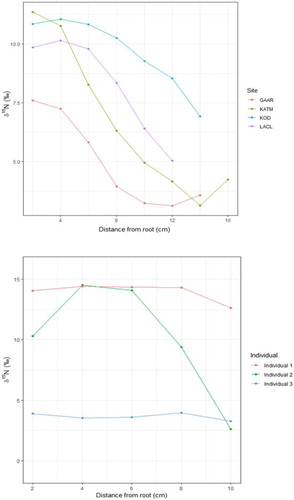
Table 1. Isotope variability within hair sections across sites. The given N is for the number of discrete hair sections sampled at each site, not the number of individual bears. The degree of variability within hair samples is a metric of the degree of diet variability within individuals and across sites. Site abbreviations are as follows: Gates of the Arctic NP – GAAR; Katmai NP – KATM; Lake Clark NP – LACL; Kodiak NWR – KOD.

		δ^15N (‰)			δ^13C (‰)
Site	N	Mean	Max	Min	Mean	Max	Min
GAAR	382	5.56	14.73	1.08	−21.98	−17.36	−23.92
KATM	168	7.69	15.94	0.61	−20.49	−14.94	−24.22
LACL	227	8.72	15.55	1.10	−20.57	−17.11	−24.15
KOD	95	12.03	15.31	2.00	−18.77	−16.69	−23.55

3.2. Isotopic dietary niche breadth estimates

For all bears pooled together across sites the dietary niche breadth estimates produced by sectioned hair samples was significantly larger than that produced from whole hair samples (Table 2). For each site, the mean dietary niche breadth estimate derived from sectioned hair data was larger than the estimate derived from whole hair data (Table 2), but the difference was only significant at GAAR and KATM. An example of the SEA_c ellipses generated for KATM bears are shown in Figure 3. The dietary niche breadth of bears from KATM and LACL derived from sectioned hair samples was nearly as large as the dietary niche breadth for the entire set of bears. Niche breadth areas determined for GAAR and KOD were significantly smaller (α = 0.05, p < 0.01).

Figure 3. Example of isotopic niche ellipses for KATM bear sectioned (black) versus whole (red) hair data.

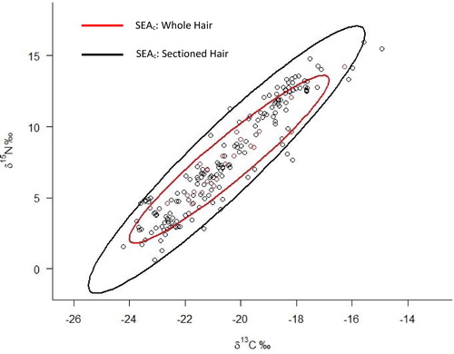
Table 2. Results of dietary niche breadth modelling. Values represent the area encompassed by the isotopic niche breadth Bayesian ellipse generated in SIBER using whole and sectioned hair data. Starred populations indicate significant differences between sectioned and whole hair estimate of SEA_b (α = 0.05, p < 0.01).

		Isotopic dietary niche breadth (‰)
		All Bears*	GAAR*	KATM*	LACL	KOD
Sectioned hair	95% CI Upper	8.56	5.90	10.03	9.52	4.09
	Mean	8.02	5.35	8.60	8.32	3.30
	95% CI Lower	7.49	4.83	7.38	7.33	2.73
Whole hair	95% CI Upper	6.81	4.73	7.14	9.35	3.65
	Mean	5.81	3.71	4.53	7.02	2.12
	95% CI Lower	5.02	2.95	3.03	5.29	1.34

4. Discussion

The use of stable isotope data from serially sectioned bear hair generated significantly larger estimates of isotopic niche breadth than whole hair data and gave a more accurate estimation of true isotopic niche breadth. This was true for the total sampled population and for half of the site-level analyses (Table 2). The overall population of bears sampled in this study occupy a wide range of habitats and have a correspondingly large range of potential diet items that span multiple trophic levels, from a variety of vegetation types such as sedges and berries, to intertidal invertebrates, multiple species of salmon, and terrestrial ungulates [24,31]. Furthermore, many of these diet items have varying seasonal abundance and availability. Our results show that the dietary variability which is captured by sectional analysis of hair is not replicated by analyzing whole hairs.

In all regions, the sectioned hair isotope data yielded larger mean estimates of isotopic niche breadth than the whole hair isotope data, and at two of the sites (GAAR and KATM) the difference was statistically significant. Two of the sites (GAAR and KOD) had relatively smaller isotopic niche breadth estimates compared to the others (LACL and KATM). Despite the bears at these two sites having a smaller breadth of resource use, the sectioned hair analysis still managed to capture more of the intra-site dietary variability.

Some bears appear to be switching seasonally from a predominantly plant-based diet (approximately −2 to 0 ‰ δ¹⁵N) to a predominantly salmon-based diet (approximately 10–12 ‰ δ¹⁵N). Salmon are a temporally limited resource in many systems but are one of the most important factors in determining brown bear size and productivity [22]. However, some bears will preferentially choose fruits over salmon when both are available, which may help the bear meet broader optimal macronutrient or micronutrient needs [32,40–42]. Thus, the complex life history and foraging behaviour of brown bears requires a sampling method which can capture the temporal variability inherent in many bear populations’ diets. The whole hair niche breadth analysis results in a loss of information about the seasonality of diet and shorter time-scale deviations in foraging ecology. Items consumed for a short time may still be vitally important for an animal's overall nutritional ecology, such as the diet of brown bears upon den emergence.

Researchers must determine the time scale of diet inference that is desired in a study, combined with the time scale of inference possible due to growth and equilibration within the tissue, and plan the experimental sampling design accordingly. Potential considerations for sampling design are the timing of seasonally available diet items and likelihood of consumption, as well as the growth rate and architecture of the tissue. A final consideration is the isotope equilibration time of the tissue. If diet switches occur more rapidly than the tissue can incorporate those changes, the resultant isotope signature in the tissue would not fully capture the diet variability and could complicate the analysis. By the same token, studies based on slow turnover tissues (e.g. muscle) may also be underestimating niche breadth. Species-specific isotope equilibration rates would be necessary to help determine the time frame of dietary integration into tissue and could help improve estimates of isotopic niche breadth.

Use of sectional analysis of sequentially grown tissues may not always be necessary to fully capture an animal's isotopic foraging niche. We can envision a scenario in which an animal has a consistent dietary source throughout the duration of tissue (e.g. hair) growth. Sectional analysis of an isotopically consistent hair will not yield a broader estimation of isotopic niche than analysis of the whole hair, as in bears from KOD. Analysis of whole hair is less time-consuming from a sample preparation perspective and is correspondingly more economical in cases where it is warranted.

The results of this study may be useful to researchers hoping to inform management of brown bears and consumers more generally. Brown bear hair is generally known to grow during a portion of the active season, approximately from May to October in healthy bears with adequate nutrition [43]. Tracking brown bear dietary niche breadth across spatial and temporal scales can allow managers to monitor the breadth of resource use within a population and identify when or where bears or other consumers may have lost access to a resource. Determining if a subpopulation of animals has a narrow dietary niche would allow wildlife managers to better conserve those dietary resources in a targeted manner during certain seasons, ensuring that consumers have access to prey without competing with human consumption of the same prey base [44,45] or prioritizing conservation of habitat which is essential to brown bear or other consumer forage species [46].

Sequentially grown tissues such as hair allow for the monitoring of diet with minimal sampling. A hair sample can be taken using passive means such as hair snares. If comparisons of niche breadth will be made across individuals, sampling should ideally occur within the same season and within as close a temporal window as is possible. The stable isotope information gained from the hair sample can be used to infer diet over the previous five to six months of hair growth, which would otherwise be nearly impossible without direct observation or more frequent sampling events. The results of this study can also be applied to any species that produces sequentially grown and metabolically inert tissues and has a diverse or seasonally changing diet.

5. Conclusions

Both SIA and Bayesian dietary niche breadth estimation methods have grown in popularity in recent years [1,47]. As this trend continues, it is necessary that users understand the limitations and best practices standards of these methods. Sectional analysis of durable, inert tissues can provide finer time scale estimates of diet and reveal seasonal variation that is not evident from whole tissue data [47–49]. The results of this study show that the use of serially sampled sequentially grown tissues can better infer a true estimate of consumer dietary niche breadth compared to whole samples of the same tissue.

Acknowledgements

The authors would like to sincerely thank C. Stricker and V. von Biela for a review of this manuscript.

Disclosure statement

No potential conflict of interest was reported by the author(s).

References

- Newsome SD, Clementz MT, Koch PL. Using stable isotope biogeochemistry to study marine mammal ecology. Mar Mamm Sci. 2010;26(7):509–572.
- Boecklen WJ, Yarnes CT, Cook BA, et al. On the use of stable isotopes in trophic ecology. Annu Rev Ecol Evol Systematics. 2011;42:411–440. doi: 10.1146/annurev-ecolsys-102209-144726
- Grey J, Jones RI, Sleep D. Seasonal changes in the importance of the source of organic matter to the diet of zooplankton in Loch Ness, as indicated by stable isotope analysis. Limnol Oceanogr. 2001;46(3):505–513. doi: 10.4319/lo.2001.46.3.0505
- McKinney MA, Iverson SJ, Fisk AT, et al. Global change effects on the long-term feeding ecology and contaminant exposures of East Greenland polar bears. Glob Chang Biol. 2013;19(8):2360–2372. doi: 10.1111/gcb.12241
- Wilkinson MJ, Yai Y, O’Brien DM. Age-related variation in red blood cell stable isotope ratios (δ13C and δ15N) from two Yupik villages in southwest Alaska: a pilot study. Int J Circumpolar Health. 2007;66(1):31–41. doi: 10.3402/ijch.v66i1.18222
- Roth JD. Temporal variability in Arctic fox diet as reflected in stable-carbon isotopes; the importance of sea ice. Oecologia. 2002;133(1):70–77. doi: 10.1007/s00442-002-1004-7
- Cerling TE, Wittemyer G, Ehleringer JR, et al. History of Animals using Isotope Records (HAIR): a 6-year dietary history of one family of African elephants. Proc Nat Acad Sci. 2009;106(20):8093–8100. doi: 10.1073/pnas.0902192106
- Hopkins JB, Koch PL, Schwartz CC, et al. Stable isotopes to detect food-conditioned bears and to evaluate human–bear management. J Wildl Manag. 2012;76(4):703–713. doi: 10.1002/jwmg.318
- Eisenmann P, Fry B, Holyoake C, et al. Isotopic evidence of a wide spectrum of feeding strategies in Southern hemisphere humpback whale baleen records. PLoS ONE. 2016;11(5):e0156698. doi: 10.1371/journal.pone.0156698
- Schwertl M, Auerswald K, Schnyder H. Reconstruction of the isotopic history of animal diets by hair segmental analysis. Rapid Commun Mass Spectrom. 2003;17(12):1312–1318. doi: 10.1002/rcm.1042
- Beltran R, Connolly Sadou M, Condit R, et al. Fine-scale whisker growth measurements can reveal temporal foraging patterns from stable isotope signatures. Mar Ecol Prog Ser. 2015;523:243–253. doi: 10.3354/meps11176
- Montanari S, Amato G. Discrimination factors of carbon and nitrogen stable isotopes from diet to hair and scat in captive tigers (Panthera tigris) and snow leopards (Uncia uncia). Rapid Commun Mass Spectrom. 2015;29(11):1062–1068. doi: 10.1002/rcm.7194
- Doll AC, Taras BD, Stricker CA, et al. Temporal records of diet diversity dynamics in individual adult female Steller sea lion (Eumetopias jubatus) vibrissae. Oecologia. 2018;188(1):263–275. doi: 10.1007/s00442-018-4173-8
- Bearhop S, Adams CE, Waldron S, et al. Determining trophic niche width: a novel approach using stable isotope analysis. J Anim Ecol. 2004;73(5):1007–1012. doi: 10.1111/j.0021-8790.2004.00861.x
- Jackson AL, Inger R, Parnell AC, et al. Comparing isotopic niche widths among and within communities: SIBER – Stable Isotope Bayesian Ellipses in R. J Anim Ecol. 2011;80:595–602. doi: 10.1111/j.1365-2656.2011.01806.x
- Hutchinson GE. Concluding remarks. Cold Spring Harb Symp Quant Biol. 1957;22:415–427. doi: 10.1101/SQB.1957.022.01.039
- Colwell RK, Futuyma DJ. On the measurement of niche breadth and overlap. Ecology. 1971;52(4):567–576. doi: 10.2307/1934144
- Machovsky-Capuska GE, Senior AM, Simpson SJ, et al. The multidimensional nutritional niche. Trends Ecol Evol. 2016;31(5):355–365. doi: 10.1016/j.tree.2016.02.009
- Rode KD, Stricker CA, Erlenbach J, et al. Isotopic incorporation and the effects of fasting and dietary lipid content on isotopic discrimination in large carnivorous mammals. Physiol Biochem Zool. 2016;89(3):182–197. doi: 10.1086/686490
- Mizukami RN, Goto M, Izumiyama S, et al. Estimation of feeding history by measuring carbon and nitrogen stable isotope ratios in hair of Asiatic black bears. Ursus. 2005;16(1):93–101. doi: 10.2192/1537-6176(2005)016[0093:EOFHBM]2.0.CO;2
- Bentzen TW, Shideler RT, O’Hara TM. Use of stable isotope analysis to identify food-conditioned grizzly bears on Alaska’s North Slope. Ursus. 2014;25(1):14–23. doi: 10.2192/URSUS-D-13-00002.1
- Hilderbrand GV, Gustine DD, Mangipane BA, et al. Body size and lean mass of brown bears across and within four diverse ecosystems. J Zool. 2018;305:53–62. doi: 10.1111/jzo.12536
- Reynolds PE, Reynolds HV, Shideler RT. Predation and multiple kills of muskoxen by grizzly bears. Ursus. 2002;13:79–84.
- Wilson RR, Gustine DD, Joly K. Evaluating potential effects of an industrial road on winter habitat of caribou in north-central Alaska. Arctic. 2014;67:472–482. doi: 10.14430/arctic4421
- Mangipane LS, Belant JL, Lafferty DJ, et al. Dietary plasticity in a nutrient-rich system does not influence brown bear (Ursus arctos) body condition or denning. Polar Biol. 2018;41(4):763–772. doi: 10.1007/s00300-017-2237-6
- Bennett AJ, Thompson WL, Mortenson DC. Vital signs monitoring plan: Southwest Alaska network. Anchorage (AK): National Park Service; 2006.
- Boggs KW, Klein SC, Grunblatt JE, et al. Landcover classes, ecoregions and plant associations of Katmai National Park and Preserve. Fort Collins (CO): National Park Service; 2003. (Natural Resource Technical Report NPS/KATM/NRTR—2003/001).
- Ferguson SH, McLoughlin PD. Effect of energy availability, seasonality, and geographic range on brown bear life history. Ecography. 2000;23(2):193–200. doi: 10.1111/j.1600-0587.2000.tb00275.x
- Barnes V, Smith R. Estimates of brown bear abundance on Kodiak Island, Alaska. Ursus. 1998;10:1–9.
- Van Daele LJ, Belant JL, Barnes VG. Ecological flexibility of brown bears on Kodiak Island. Ursus. 2012;23(1):21–29. doi: 10.2192/URSUS-D-10-00022.1
- Van Daele MB, Robbins CT, Semmens BX, et al. Salmon consumption by Kodiak brown bears (Ursus arctos middendorffi) with ecosystem management implications. Can J Zool. 2013;91(3):164–174. doi: 10.1139/cjz-2012-0221
- Deacy WW, Armstrong JB, Leacock WB, et al. Phenological synchronization disrupts trophic interactions between Kodiak brown bears and salmon. Proc Natl Acad Sci USA. 2017;114(39):10432–10437. doi: 10.1073/pnas.1705248114
- Taylor WP Jr, Reynolds HV III, Ballard WB. Immobilization of grizzly bears with tiletamine hydrochloride and zolazepam hydrochloride. J Wildl Manag. 1989;53:978–981. doi: 10.2307/3809598
- Elgmork K, Riiser H. Hair structure of brown bears (Ursus arctos L.) from North America and Scandinavia. Can J Zool. 1991;69(9):2404–2409. doi: 10.1139/z91-337
- O’Connell TC, Hedges REM, Healey MA, et al. Isotopic comparison of hair, nail and bone: modern analyses. J Archaeol Sci. 2001;28(11):1247–1255. doi: 10.1006/jasc.2001.0698
- Cerling TE, Wittemyer G, Rasmussen HB, et al. Stable isotopes in elephant hair document migration patterns and diet changes. Proc Natl Acad Sci USA. 2006;103(2):371–373. doi: 10.1073/pnas.0509606102
- Neuberger FM, Jopp E, Graw M, et al. Signs of malnutrition and starvation—reconstruction of nutritional life histories by serial isotopic analyses of hair. Forensic Sci Int. 2013;226(1–3):22–32. doi: 10.1016/j.forsciint.2012.10.037
- Rogers MC, Peacock E, Simac K, et al. Diet of female polar bears in the southern Beaufort Sea of Alaska: evidence for an emerging alternative foraging strategy in response to environmental change. Polar Biol. 2015;38(7):1035–1047. doi: 10.1007/s00300-015-1665-4
- R Core Team. R: A language and environment for statistical computing. Vienna, Austria: R Foundation for Statistical Computing; 2017. Available from: https://www.R-project.org/.
- Rode KD, Robbins CT. Why bears consume mixed diets during fruit abundance. Can J Zool. 2000;78(9):1640–1645. doi: 10.1139/z00-082
- Fortin JK, Farley SD, Rode KD, et al. Dietary and spatial overlap between sympatric ursids relative to salmon use. Ursus. 2007;18(1):19–29. doi: 10.2192/1537-6176(2007)18[19:DASOBS]2.0.CO;2
- Erlenbach JA, Rode KD, Raubenheimer D, et al. Macronutrient optimization and energy maximization determine diets of brown bears. J Mamm. 2014;95(1):160–168. doi: 10.1644/13-MAMM-A-161
- Jacoby M, Hilderbrand G, Servheen C, et al. Trophic relations of brown and black bears in several western North American ecosystems. J Wildl Manag. 1999;63(3):921–929. doi: 10.2307/3802806
- Peirce JM, Otis EO, Wipfli MS, et al. Interactions between brown bears and chum salmon at McNeil River, Alaska. Ursus. 2013;24:42–53. doi: 10.2192/URSUS-D-12-00006.1
- Brockman CJ, Collins WB, Welker JM, et al. Determining kill rates of ungulate calves by brown bears using neck-mounted cameras. Wildl Soc Bull. 2017;41(1):88–97. doi: 10.1002/wsb.733
- Fish US, Service W. Final conservation strategy for the grizzly bear in the Greater Yellowstone Area. Missoula (MT): Developed by the Interagency Conservation Strategy Team; 2007.
- Ben-David M, Flaherty EA. Stable isotopes in mammalian research: a beginner’s guide. J Mamm. 2012;93(2):312–328. doi: 10.1644/11-MAMM-S-166.1
- Milakovic B, Parker KL. Quantifying carnivory by grizzly bears in a multi-ungulate system. J Wildl Manag. 2013;77(1):39–47. doi: 10.1002/jwmg.434
- Rossman S, Ostrom PH, Gordon F, et al. Beyond carbon and nitrogen: guidelines for estimating three-dimensional isotopic niche space. Ecol Evol. 2016;6(8):2405–2413. doi: 10.1002/ece3.2013