The low-volatility effect in African frontier equity markets

ABSTRACT

This study investigated the extent to which the low-risk anomaly is present in a pooled sample of nine African frontier equity markets from March 2004 to July 2023. Portfolio-level analysis was used to investigate the total stock returns of equally weighted quintile portfolios sorted on historical volatility. The presence of a monotonic relationship between historical volatility and subsequent returns was evaluated using monotonicity tests, controlling for possible mediating variables. The results revealed evidence of a statistically significant low-volatility premium, except during bull markets. These findings imply that investors can expect to earn higher returns by allocating to stocks with lower historical volatility, but only during bear markets. These results hold for realistic portfolio construction constraints, such as (il)liquidity and high transaction costs.

KEYWORDS:

• low-risk
• low-volatility
• African frontier markets
• transaction costs
• liquidity constraints
• anomaly

1. Introduction

Traditional finance theory contends that higher risk is associated with higher expected stock returns. This higher-risk, higher-reward expectation was conceptualised in the development of Capital Market Theory. In other words, investors should demand and expect higher returns as compensation for taking on higher levels of risk. The Capital Asset Pricing Model (CAPM), one of the key models developed under Capital Market Theory, formalises this concept by proposing that the expected return of an asset should be proportional to its systematic risk, as measured by its beta coefficient relative to the overall market portfolio. However, in the 1970s, empirical studies began to cast doubt on the seemingly rational positive risk-return assumption (Black et al., 1972; Haugen & Heins, 1975; Fama & French, 1992). These studies found the risk-return relationship to be either flat, less than predicted, or even negative. This peculiar phenomenon has been termed the low-risk anomaly.

Investing in equity markets in emerging economies is typically associated with higher volatility. Investors who invest in these markets consequently expect to be rewarded for the additional risk they assume (Bekaert et al., 1998). If the low-risk anomaly holds true, then investors have no basis to expect additional returns from higher-risk investments. In fact, investors should be willing to pay more for low-risk stocks compared to high-risk ones given their higher return profile.

Evidently, the low-risk anomaly contradicts traditional investment theories. This paradox questions the effectiveness of asset pricing models that assume a positive risk-return relationship. These models include the CAPM (Sharpe, 1964) and various other multifactor models such as the Fama and French three-factor model (Fama & French, 1993), the Carhart four-factor model (Carhart, 1997), and the Fama and French five-factor model (Fama & French, 2015).

Studies have found evidence of the low-risk anomaly in emerging and developed markets alike (Baker & Haugen, 2012; Blitz et al., 2013; Hsu et al., 2013; Blitz et al., 2019). However, as far as could be determined, there are no studies that have investigated whether the anomaly extends to frontier markets. This pragmatic study aims to fill this gap. Index providers distinguish between “frontier” and “emerging” markets for the benefit of global investors (Quisenberry & Griffith, 2010). Emerging markets are typically countries that are in the process of developing, where frontier markets are less advanced economies, typified by smaller, less developed, and typically more volatile stock markets (Quisenberry & Griffith, 2010). The distinction is useful, as it provides valuable insights into the relative investability of these economies.

Although the low-risk anomaly has been well documented, there is still considerable uncertainty about whether the anomaly holds in all markets and under different stock market conditions. For example, Haugen and Heins (1975) suggested that high-risk stocks will only underperform during bear markets, due to their increased sensitivity to market circumstances. This proposition was termed the bull-bear market hypothesis. Similarly, some scholars have claimed that the anomaly could be explained by sector-, size-, and/or country effects (Bali & Cakici, 2008; Beveratos et al., 2017).

The purpose of this study was thus to expand the existing research to nine frontier African equity markets by testing for a negative monotonic risk-return relationship in the stocks listed in these markets. Although there are many different proxies for risk (Blitz & Van Vliet, 2007; Baker et al., 2011; Steyn & Theart, 2019), the authors used realised (or historical) volatility as the risk measure to evaluate the low-risk anomaly. This methodological decision led to the interchangeable use of the terms low-risk and low-volatility (Blitz & Van Vliet, 2007; Blitz et al., 2013). Blitz et al. (2013) also used volatility as the main measure of risk and evaluated beta and mean absolute deviation as well. Although their study concluded that the low-risk anomaly is robust for changes in the risk measure used, it was most profitable when volatility was employed as the risk proxy.

To address the gap in the research, four specific research objectives were formulated in the current study. The first (i) related to establishing whether there is a definitive risk-return trade-off in frontier African equity markets. The second research objective (ii) called for an investigation into the degree to which any low-volatility premium is affected by liquidity, sector, country, holding period, and size effects. In recognition of the potential distortion of returns by trading fees, settlement charges, and equity custody costs, the analysis was re-run for a range of effective trading cost levels. The authors also determined (iii) whether there is a difference in the nature of the low-volatility premium during different market states, i.e., during bull and bear markets. The fourth and final research objective (iv) investigated whether the low-volatility anomaly is present within countries when returns are measured in local currencies. Thus, this study sought to uncover robust evidence on the true character of the risk-return relationship in the African frontier equity market context. Given the characteristically high expected returns and volatility of frontier markets, it is plausible that the relationship between risk and return in these markets differs from that observed in more mature markets.

Insights gained from the output of the study could potentially shed light on the investor behaviour of these smaller equity markets relative to the large and more advanced markets. Investors and investment professionals in these markets could benefit from this study's findings, as it could guide their investment choices. Market practitioners, particularly those interested in investment product design, could gain from the knowledge of the performance of the low-volatility risk factor, as well as the perceptions relating to the impact of market microstructure effects. To the extent that the low-risk effect is related to risk-seeking investor behaviour among African investors, the results may also be of interest to regulatory authorities, who may contemplate measures to mitigate potentially destabilising outcomes.

The sections that follow include a brief overview of the low-volatility literature and the research design employed. Thereafter, key results are presented and discussed. Finally, the implications of the findings are reviewed in relation to the investment decision-making process and possible investment opportunities in the frontier African equity market.

2. Review of relevant literature

2.1. Background to the risk-return trade-off

The expectation that greater levels of risk should result in higher returns is intuitive and appealing from an investment standpoint. Investors are generally assumed to be risk-averse, therefore, they will only be willing to take on higher levels of risk if they are compensated with higher expected returns. Conversely, assets with lower risk levels should theoretically offer lower expected returns. The suggestion of how risk-averse investors should behave can be traced back to 1952 when Markowitz introduced the MPT in his seminal article “Portfolio Selection” (Markowitz, 1952). Markowitz suggested there is an inherent trade-off between risk and return that arises due to the behaviour of risk averse investors. Thus, according to the MPT, an ‘efficient frontier’ can be constructed comprising of optimal portfolios that maximise return for each level of risk.

Building on the principles set forth in MPT, several theories and asset pricing models were subsequently developed. Capital Market Theory simplified Markowitz’ theory and differentiated between systematic and non-systematic risk (Sharpe, 1964). This theory led to the development of the Capital Asset Pricing Model (CAPM) which is a static (single-period) model that predicts the required return of an asset or portfolio based solely on its sensitivity to market movements (beta) compared to the risk-free rate and the market’s expected return. The Arbitrage Pricing Theory also assumes a positive risk-return relationship, but unlike the CAPM, it incorporates a number of variables that integrate systematic risk (Ross, 1976). Similarly, other multifactor models have added extra variables but, nevertheless, assume a positive risk-return relationship. These models include the Fama and French three-factor model (Fama & French, 1993), the Carhart four-factor model (Carhart, 1997), and the Fama and French five-factor model (Fama & French, 2015).

Not long after the CAPM model had been developed, empirical studies challenged the validity of the model’s predictions. Early studies found the risk-return relationship to be either non-existent, less than predicted, or even negative. Haugen and Heins (1975) reported a negative relationship between risk and return in United States (US) stock and bond markets from 1926 to 1971. However, Black et al. (1972) and Fama and MacBeth (1973) found a positive relationship between beta and average return during the period 1926–1966 and 1926–1968, respectively. Black et al. (1972) argued that the strength of this relationship was less than predicted by the CAPM. These scholars specifically observed that the CAPM understated the return of low-beta stocks in the US equity market. Moreover, Fama and French (1992) noted that this simple positive relationship between beta and average return disappeared during the period between 1963 and 1990. The authors observed that the different outcome could be due to the sample period selected but noted that the positive relation between beta and average returns documented in earlier studies disappears when controlling for size from 1941 to 1965.

2.2. Empirical evidence

Several studies indicated a negative relationship between historical volatility and subsequent stock returns in the US. Haugen and Baker (1991) illustrated that, relative to a market capitalisation weighted benchmark, it was low-risk shares that produced higher returns from 1972 to 1989. There was renewed interest in the topic amongst scholars in the US in the early 2000s when Goyal and Santa-Clara (2003) presented evidence of a significant positive correlation between average stock variance and the return for US stocks over the period 1963 to 1999. However, Bali et al. (2005) challenged this conclusion and reported no relationship between average stock volatility and value-weighted portfolio returns in the US market. The authors attributed the findings of Goyal and Santa-Clara (2003) to liquidity and small-size effects.

Further confirmation of a negative risk-return relation in the US stock market was provided by Jagannathan and Ma (2003), and Blitz and Van Vliet (2007). Similarly, Ang et al. (2006) document no evidence of a positive risk-return relationship. The authors reported that shares with high levels of risk (either systematic or idiosyncratic) had very low average returns for the period 1986 to 2000.

The low-volatility anomaly has been shown to persist over time. Blitz and Van Vliet (2007), for example, subdivided the sample period into two 10-year time periods for the US and other developed markets. The study documents evidence of the low-volatility anomaly for the years 1985 to 1995 and an even stronger volatility effect for the period 1996 to 2005. Furthermore, evidence of the anomaly has not only been found during times of market downturns, but also during market upswings (Baker et al., 2011; Li, 2013). This is a particularly significant discovery considering that the bull-bear market hypothesis predicts that low beta stocks (stocks with low systematic risk exposure) will only outperform during bear markets.

Although Haugen and Heins (1975) presented evidence in support of the bull-bear market hypothesis, other studies have indicated that the low-volatility anomaly exists in both bull and bear markets (Baker et al., 2011; Li, 2013). In an investigation that covered 43 developed and emerging stock markets, Fifield et al. (2020) documented a positive risk-return relation when returns are high and during bear markets, and a negative relation at low return levels and during bull markets.

Asness et al. (2014) provided evidence that the anomaly persists across industries, which implies that a low-risk filter can be useful not only for stock selection but also for industry selection decisions. These researchers show an inter-industry anomaly, or put differently, an anomaly that exists across industries. Baker et al. (2014) created sector-neutral portfolios and found that the low-risk anomaly persisted even after controlling for industry biases. Since the sector-neutral portfolios did not impact the findings, it can be assumed that the low-risk anomaly was equally present in all the industry sectors under investigation. This result provides indirect evidence of an intra-industry anomaly. If a perfect intra-anomaly exists, neutralising for industry biases would essentially be unnecessary.

The low-volatility anomaly has not been limited to a specific market or a specific region (Blitz & Van Vliet, 2007; Yamada & Uesaki, 2009). Blitz and Van Vliet (2007) uncovered a low-volatility anomaly in the US, Japanese, and European markets from 1986 to 2006. Likewise, Yamada and Uesaki (2009) found evidence of a low-volatility anomaly in various developed equity markets from 1990 to 2008 and in the Japanese market from 1975 to 2008. Baker and Haugen (2012), Blitz et al. (2013) and Hsu et al. (2013) specifically investigated the anomaly in emerging markets compared to developed markets and found support for of an anomaly that is robust across markets with varying degrees of economic development.

2.3. Possible explanations for the low-risk anomaly

There are several potential reasons for the existence of the low-volatility anomaly. Black (1972) suggested leverage constraints as a possible explanation for the lack of empirical evidence for the CAPM. For many investors, the ability to engage in short selling or utilise leverage is constrained by either their investment mandate or limited resources. Frazzini and Pedersen (2014) proposed that the anomaly is partly due to investors who try to increase their expected returns by over-allocating to high-risk shares in lieu of using leverage, thereby bidding up their prices. This additional demand for high-risk shares results in a flattening of the risk-return relation.

Similarly, limits to arbitrage, such as constraints on short selling, transactions cost and liquidity, could explain the continued existence of the low-risk anomaly (Blitz et al., 2014). Indeed, Li et al. (2014) showed that the high transaction costs associated with attempting to implement a long-short low-volatility portfolio erode the outperformance significantly. The authors documented that the abnormal returns of the strategy tend to be concentrated in small shares with lower liquidity, which makes the impact of market frictions larger.

Others have suggested that the observed low-volatility anomaly could be due to the irrational behaviour of market participants (see, for example, Blitz & Van Vliet, 2007; Baker et al., 2011; Blitz et al., 2014). This explanation infers that the outperformance of the low-volatility effect could be a manifestation of an irrational preference for high-volatility assets, which is due to psychological factors that influence the investment decisions of investors. For example, a preference for lottery-like payoff profiles will increase the demand for higher volatility shares relative to low volatility shares (Kumar, 2009; Fong, 2013). Kumar (2009) furthermore showed that the demand for lottery-type shares (high-volatility) increases during economic downturns, which will explain the higher expected return of low-volatility. Fong (2013) demonstrated that risk-seeking investors drive this demand for lottery-type shares. Baker and Haugen (2012) contended that this type of risk-seeking behaviour exhibited by institutional investors is not necessarily irrational, as the asymmetric nature of their compensation structures incentivises them to concentrate on high-risk assets.

On a related note, Wang et al. (2017) documented evidence that the inverse risk-return relation is stronger among shares where investors face a capital loss, i.e., shares that have fallen in price. Indeed, for shares where investors face a capital gain, the authors note a positive association between risk and return. This result supports the theory that investors become more risk-seeking when facing a potential loss and are therefore more willing to increase their demand for higher risk shares.

As far as could be determined, South Africa is the only African country in which the low-risk anomaly has been investigated. Van Rensburg and Robertson (2003) recorded a low-beta anomaly over the period 1990 to 2000 in the South African equity market. Similarly, Steyn and Theart (2019) presented empirical evidence in favour of a low-volatility anomaly on the Johannesburg Stock Exchange (JSE), using risk-adjusted returns as a gauge of performance. Oladele and Bradfield (2016; 2018) assessed the profitability of low-volatility investment strategies on the JSE and found support for an investment case that incorporates low-volatility strategies. In a more recent study, Seetharam (2022) used four different risk measures and found evidence of a low-risk anomaly in South Africa from 1990 to 2016; however, the anomaly disappeared for most risk measures after controlling for size and value effects.

The reviewed literature provides a significant body of empirical evidence of a negative relationship between risk and return over different time periods, during different market states, after controlling for possible sector or size effects, and within both developed and emerging markets. There are, however, minimal studies including frontier markets, and none specifically on African frontier markets. Global investors in African stock markets face several challenges, including weak accounting and disclosure standards, noise trading, differences in social and cultural practices, high liquidity risk, restrictions on short-selling, and lack of information transparency (Boamah et al., 2016; Asongu 2017; Wu et al., 2019). Nonetheless, these markets offer significant diversification advantages stemming from their low correlation with other stock markets (Alagidede, 2009) and potentially higher market risk premiums compared to developed and emerging markets (Boamah et al., 2016). Therefore, it is important to examine whether investors in frontier African markets demonstrate similar investment behaviours to those of investors in developed and other emerging stock markets. In the following section, details are presented on how these gaps in the extant literature were addressed.

3. Research design

3.1. Data

A judgement-based sampling process was followed in this pragmatic study to select the sample of stocks. To be included in the sample for a given month, a stock had to form part of the top 150 stocks (based on its US dollar market capitalisation) listed on the list of African stock exchanges included in the study (see below). Due to its relative size, breadth, and depth, South Africa was excluded from the analysis as it would have dominated the sample. South Africa is also classified as an ‘emerging’ market rather than a ‘frontier’ market (Serkin, 2015).

Following Boamah (2017), selected stocks were limited to nine African frontier markets, namely Egypt, Morocco, Mauritius, Nigeria, Kenya, Tunisia, Ivory Coast, Ghana, and Botswana. These countries were chosen based on global investor accessibility and the availability of price and volume data. Monthly US dollar price data was collected from Bloomberg for the period 1 March 2004 to 31 July 2023. The sample period was chosen to cover multiple market cycles, incorporating major disruptive events like the Global Financial Crisis and the COVID-19 pandemic. Further considerations in selecting the timeframe included data availability, ensuring a sufficient sample size, and adequate liquidity. To address survivorship bias, the sample included stocks that were delisted during the sample period. If a certain stock was delisted, its return was calculated up until the last full month prior to delisting. Using the returns from the last complete month's data only (i.e., ignoring the intra-month returns in the final month of its listing) may be criticised for look-ahead bias. In addition, it may be seen to be positively biasing the results by avoiding the negative impact of bankruptcies (i.e., −100% returns) in the month of delisting. However, in this study it is assumed that any impending delisting event would be known by the preceding month-end rebalancing date. This is a realistic assumption as delistings, even in bankruptcy cases, are typically well-telegraphed and communicated to investors ahead of time. Therefore, the market price movements should already reflect this information in the months leading up to the actual delisting date. In addition, the negative 100% return in this period would only apply to bankruptcies. A random sample of delistings was drawn and only 10% were found to be due to this type of delisting event. Ultimately, the overall expected impact of the chosen methodology was deemed to be negligible.

Following other studies on frontier markets (Boamah, 2017; Zaremba & Maydybura, 2019), a pooled sample approach across a number of countries helped address the small sample size problem arising when individual countries are analysed in isolation. To be included in the pooled sample, a listed company needed to have both the return in month t and the market capitalisation in month t-1 available. Additionally, a stock had to have at least 36 months of price history. Table 1 provides an overview of the sample at the end of the research period (March 2004 to July 2023).

Table 1. Overview of sample at end of sample period.

	Number of stocks	Mean market capitalisation (US$ Million)
Egypt	120	626
Nigeria	60	849
Morocco	54	1,372
Kenya	29	624
Ivory Coast	23	363
Tunisia	21	310
Mauritius	16	445
Botswana	12	350
Ghana	11	187
Total	346

Source: Bloomberg as at July 2023. The sample period is 01/03/2004 to 31/07/2023

Although Egypt had the largest number of stocks in the sample (120), Morocco had the highest average market value (US$1,372 million). This process ensured that the aggregate sample was large enough to construct diversified quintile portfolios and conduct empirical tests. The local currency analysis within individual countries was limited to Egypt, Nigeria, Morocco, and Kenya. This constraint is due to the small number of listed shares with reasonable liquidity in the remaining markets. For the local currency analysis within selected countries, no limit was placed on the number of shares included in the sample.

Monthly total returns were calculated after the necessary adjustments had been made for stock splits, stock repurchases, dividends, and other corporate actions. Extreme observations in individual share returns may disproportionately affect constructed portfolio returns. As such, it was necessary to winsorize the return data to trim the extreme outliers to more reasonable values. Following previous low-volatility researchers Jordan and Riley (2013), monthly returns across the entire sample were winsorized at the 0.5% level by converting the top 0.5% of values to the 99.5th percentile and the bottom 0.5% of values to the 0.5th percentile level.

3.2. Calculation of sorting variable

Following many other low-volatility studies (Blitz & Van Vliet, 2007; Yamada & Uesaki, 2009; Blitz et al., 2013; Steyn & Theart, 2019), the historical volatility as measured by standard deviation was used as the sorting variable. Historical volatility is a measure of total risk as it captures both systematic and idiosyncratic risk components. The standard deviation on the stock level was calculated on a monthly basis over a 36-month look-back period by following Equation (1)(1) $\mathrm{S}{\mathrm{D}}_{\mathrm{i}}=\sqrt{{\displaystyle \frac{1}{n-1}\sum _{t=1}^n{(x_{\mathrm{it}}-{\overline{x}}_i)}^2}}$(1) : (1) $\mathrm{S}{\mathrm{D}}_{\mathrm{i}}=\sqrt{{\displaystyle \frac{1}{n-1}\sum _{t=1}^n{(x_{\mathrm{it}}-{\overline{x}}_i)}^2}}$(1)

where:

SD_i = Standard deviation of stock i;

n = number of observations in the look-back period;

x_it = return observation of stock i in month t;

$\overline{x}$_i = stock i’s arithmetic mean rate of return over the look-back period.

3.3. Quintile portfolio construction

Equally weighted quintile portfolios were constructed by grouping stocks that had similar individual volatilities. The stocks with the highest observed risk measure were allocated to the high-risk quintile portfolio (P1), and the stocks with the lowest observed risk measure were assigned to the low-risk quintile portfolio (P5). Portfolios were rebalanced monthly, and the equal-weighted portfolio returns for each quintile portfolio were then calculated and recorded.

An equal-weighting scheme was chosen to increase diversification and lessen the impact of stock-specific reversals. In line with similar studies, the impact of transaction costs was initially ignored (Blitz & Van Vliet, 2007; Baker et al., 2011; Steyn & Theart, 2019). However, given that frontier African markets are characterised by high levels of transaction costs (Soumaré, 2020), and given the potential return-distorting effects related to charges for trading, settling, and custody of equity shares, the analysis was repeated for various levels of effective trading costs.

Similarly, it could be argued that the continued presence of a low-volatility effect may be due to market frictions such as (il)liquidity, which hampers the ability of trading strategies designed to profit off the anomaly. The potential effect of liquidity on the presence of the low-volatility effect was tested by employing a liquidity cap measure used by Bailey and Gilbert (2007). This liquidity constraint measure is based on the way investment managers deploy capital relative to expectations about market volumes traded. If it is assumed that investors require at least 10 trading days to fully liquidate their position (Bailey & Gilbert, 2007), 50% of historical monthly traded volumes can then be used as a liquidity constraint. For a share to be considered eligible, the required investment amount must not exceed the liquidity cap established for that particular share. This limit is then applied to different portfolio sizes to gauge the impact of constraining the investable universe relative to the average position size. Assuming each quintile portfolio contains 30 equally weighted shares, the position size of each share is roughly 3.33%. This position size is then applied to various portfolio sizes (ranging from US$10,000 to US$100 million) to determine the dollar investment in each share. For example, a US$100 million portfolio would have an average position size of US$3.33 million. A share would then need an average monthly traded value of at least US$6.66 million (two times the position size) to be included in the investable universe for this portfolio. Stated differently, 50% of the average monthly traded value over the previous 12 months is used as the liquidity cap. Therefore, an average monthly traded value of at least US$6.66 million is needed for the 50% cap to meet the position size limitation for a US$100 million portfolio. This approach effectively facilitated the development of a liquidity constraint based on the available share price and trading volume data.

As sector or country concentration can have a substantial impact on the performance of quintile portfolios, the analysis was repeated by creating country and sector-neutral portfolios. In line with Rouwenhorst (1999) and Van der Hart et al. (2003), country (or sector) neutral portfolios were thus created by distributing the shares from a specific country (or sector) uniformly across the quintile portfolios. In addition, the impact of the size effect was independently evaluated by creating size-neutral portfolios. This was done by using the median market capitalisation in the cross-section of the sample as a breakpoint. The stocks were first sorted across the two size groups and then aggregated into quintile portfolios based on historical volatility. In addition to monthly rebalancing periods, the analysis was repeated for quarterly and semi-annual holding periods.

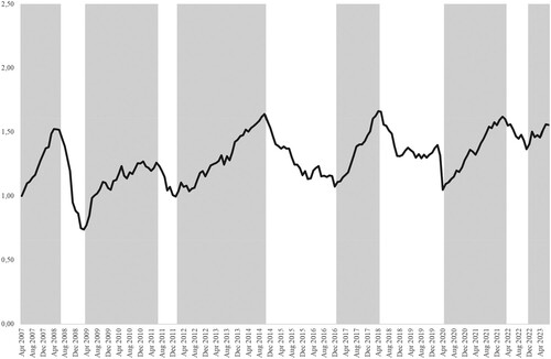
Lastly, the sample period was stratified into bull and bear periods based on the performance of the equally weighted benchmark. Haugen and Heins (1975) highlighted the potential of the nature of the empirical result to be affected by the economic state of the market being sampled. To denote the start of a bear market, the equally weighted benchmark (EBM) had to have two consecutive months of negative returns. This definition aligns with Chauvet and Potter (2000) who defined bear markets as those that correspond to periods of falling market prices, and bull markets as those that match rising market prices. Figure 1 displays shaded bull market periods, whereas unshaded sections denote bear market periods. A total of 122 months were included in the bull market sections and bear markets covered 74 months in total. This process allowed for the evaluation of Haugen and Heins’ (1975) bull-bear market hypothesis.

Figure 1. Cumulative performance of the EBM over the sample period.

(Bull market periods are shaded. Unshaded sections denote bear market periods.)

3.4. Monotonicity tests

Statistical tests of monotonicity are reasonably robust methods of evaluating asset-pricing models (Patton & Timmermann, 2010). Using the non-parametric tests developed in Patton and Timmermann (2010), it is possible to determine monotonicity at a given level of statistical significance. The Monotonic Relation (MR) assessment was designed to test the hypothesis that there is a monotonic relation between expected returns and some characteristic that, in theory, should earn a risk premium.

The MR test was employed to assess whether there was a monotonic relation between historical volatility and subsequent total stock returns across portfolio sorts. There are several benefits of using this test, as opposed to attempting to explain ex-post returns by means of regression analysis. Monotonicity implies that variables are moving in the same direction, but unlike a linear relationship, monotonicity does not require a constant rate of change. One benefit of the MR test is that it is non-parametric and relatively straightforward to implement using bootstrap techniques. Therefore, there is no requirement for a linear relationship between the sorting variable and expected returns, nor is it necessary to make distributional assumptions about returns. Under the null hypothesis, expected returns are equal or slightly declining from P1 to P5, but under the alternative, the returns are monotonically increasing. For this reason, high-volatility shares were sorted in P1 and low-volatility shares in P5. A bootstrap p-value of less than 0.05 would lead to the conclusion that the null hypothesis can be rejected in favour of a monotonically increasing association across quintile portfolios and therefore a negative risk-return relationship.

4. Presentation and analysis of results

4.1. Portfolio-level analysis

The descriptive statistics of the volatility-sorted quintile portfolios are presented in Table 2. The mean monthly returns display a pattern of increasing returns from high- to low-volatility portfolios. However, only the high-volatility quintile portfolio mean return is statistically significant. The mean monthly return of the long-short portfolio (Low minus High) of 1.31% is notably higher than any of the monthly returns of the quintile portfolios and was statistically significant at the 1% level.

Table 2. Summary statistics of the volatility sorted quintile portfolios.

	Quintile Portfolios
	1 (High)	2	3	4	5 (Low)	Low minus High	EBM
Mean monthly return	−1.20%***	−0.51%	−0.23%	−0.03%	0.11%	1.31%***	0.34%
Annualised return	−15.89%	−8.10%	−3.93%	−1.37%	0.64%	14.88%	2.94%
Annualised standard deviation	23.14%	20.64%	15.37%	13.84%	11.64%	19.17%	14.85%
Adjusted Sharpe ratio	− 0.79	− 0.47	− 0.34	− 0.18	− 0.03	0.77	0.13
Average monthly turnover	10.2%	14.4%	14.4%	13.5%	7.6%

Note: The Low minus High portfolio displays the results of buying the low volatility portfolio and shorting the high volatility portfolio on a monthly basis. The EBM is an equally weighted benchmark portfolio consisting of all the shares in the sample, rebalanced monthly. The adjusted Sharpe ratio shows the Sharpe ratio modified to account for the potential distorting effects relating to skewness and kurtosis. All returns are expressed in US dollars. The mean monthly returns were tested for statistically significant difference from zero.

*** indicates the 1% level of significance.

A similar linear pattern is observed for the compounded annual returns, where the high volatility portfolios underperformed the low-volatility portfolios. There appears to be a persistence in observed volatility, where the realised standard deviation of the quintile portfolios decreases monotonically from high- to low-volatility portfolios. The volatility of the lowest volatility portfolio (Q5) of 11.64% is lower than the EBM (14.85%), and both are much lower than the volatility of the highest volatility portfolio (Q1), which is 23.14%. This result is similar to the pattern Steyn and Theart (2019) found in the South African market over the period July 2004 to September 2018. Moreover, the average monthly turnover shows that the extreme quintiles have lower turnover rates compared to the other portfolios. This result also suggests that there is a persistence in volatility. High-volatility stocks tend to remain high-volatility stocks and low-volatility stocks stay low-volatility stocks. If volatility levels tend to persist, it means that investors can potentially use a stock's historical volatility as a predictor of its future volatility. This predictability can aid in risk management and portfolio construction decisions. In addition, the predictability of volatility levels could potentially challenge the notion of market efficiency, as investors may be able to exploit this predictability to generate abnormal returns.

Figure 2 shows an inverse linear relationship of the adjusted Sharpe ratios across the volatility-sorted quintile portfolios. High-volatility stocks produce lower risk-adjusted returns compared to low-volatility stocks. The long-short portfolio generated a much higher adjusted Sharpe ratio (0.77) than any of the quintile portfolios or the EBM.

Figure 2. Adjusted Sharpe ratio for volatility sorted quintile portfolios, the long-short portfolio (Low minus High), and the equally weighted benchmark (EBM).

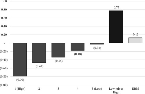
This finding contradicts the traditional finance theory that higher risk should be compensated with higher returns. Instead, it suggests that lower-risk (low-volatility) stocks offer better risk-adjusted returns than their higher-risk (high-volatility) counterparts. Investors may need to reconsider their investment strategies and portfolio construction approaches. A focus on low-volatility stocks could potentially offer better risk-adjusted returns compared to high-volatility stocks. These results may motivate researchers to investigate behavioural finance explanations within the context of African frontier equity markets, such as investor overconfidence or preferences for lottery-like payoffs (Kumar, 2009), which could potentially contribute to the underperformance observed in high-volatility stocks.

4.2. Transaction costs and liquidity cap

Table 3 illustrates the impact of incorporating transaction costs at the monthly rebalancing dates. The analysis reveals that the long-short portfolio's mean monthly returns are demonstrably positive and statistically significant at the 1% level, aligning with a more realistic representation of investment outcomes. However, at the 200bps level, the positive return is only significant at the 5% level. This finding implies that higher transaction costs do not necessarily impact the existence of the low-volatility anomaly. However, as the effective transaction costs increase, there is a deterioration in the profitability of the long-short portfolio. Nonetheless, even at the 200-basis point (bps) level, the mean monthly return is still positive and statistically significant. The results highlight that the negative risk-return relation across volatility-sorted portfolios remains in place in the presence of high transaction costs. This outcome does not fully align with Li et al. (2014) who found that high transaction costs completely erode the profitability of a long-short low-volatility strategy.

Table 3. Returns of volatility-sorted portfolios at various levels of effective transaction costs.

Transaction costs	Mean monthly return: Portfolio 1 (High)	Mean monthly return: Portfolio 5 (Low)	Long -short portfolio
Zero	−1.20%***	0.11%	1.31%***
50bps	−1.15%***	0.07%	1.23%***
100bps	−1.10%**	0.04%	1.14%***
150bps	−1.05%**	0.00%	1.05%***
200bps	−1.00%**	−0.04%	0.96%**

***, ** denote significance at the 1% and 5% level, respectively.

The persistence of the negative risk-return relationship, despite high transaction costs, could be seen as an indication of market inefficiency. If the market was truly efficient, arbitrageurs would exploit this anomaly, and the transaction costs would eventually eliminate the mispricing. However, there may be limits to arbitrage that prevent investors from fully exploiting the negative risk-return relationship, regardless of the level of transaction costs. The practical constraints against implementing short sale transactions may hamper executing a profitable trading strategy in the considered frontier African equity markets. Furthermore, structural factors specific to these markets may contribute to the persistence of the negative risk-return relationship, even when transaction costs are high.

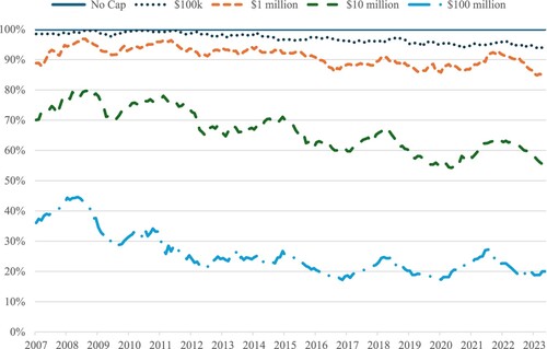
Figure 3 displays the impact of the liquidity cap on the proportion of the investable universe for various portfolio sizes. Portfolio sizes of more than US$10 million are quite restricted in terms of the liquid opportunity set available. For a US$100 million portfolio the liquidity cap restricted the universe to between 20% and 45% relative to no liquidity constraint.

Figure 3. Proportion of shares available for investment with liquidity cap.

The impact of the constrained investment universe on the low-volatility effect is displayed in Table 4 and Figure 4. The pattern of the return differential of the high- and low-volatility quintile portfolios is clearly affected by the liquidity cap. The extreme quintile portfolio returns for portfolios up to US$1 million are very similar. The pattern changes, however, when portfolio sizes reach US$10 million and larger. The difference between the high- and low-volatility portfolios increases, and from Figure 4, it appears that it is mainly driven by larger losses in the high-volatility portfolio.

Figure 4. Average monthly returns for all portfolios.

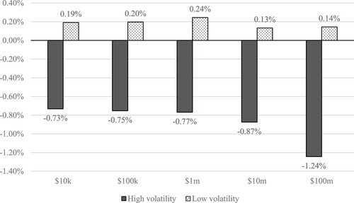
Table 4. Results from tests for monotonicity in returns across volatility-sorted portfolios at various levels of portfolio size.

Portfolio size	Mean monthly return: Portfolio 1 (High)	Mean monthly return: Portfolio 5 (Low)	Low minus High	MR test bootstrap p-value
USD10,000	−0.73%*	0.19%	0.92%**	0.028
USD100,000	−0.75%*	0.20%	0.95%**	0.043
USD1 million	−0.77%*	0.24%	1.01%**	0.104
USD10 million	−0.87%*	0.13%	1.01%**	0.012
USD100 million	−1.24%**	0.14%	1.39%***	0.034

***, **, * denote significance at the 1%, 5% & 10% level, respectively.

The monotonicity test of Patton and Timmermann (2010) allows for statistical testing of the monotonic relation across different volatility-sorted portfolios generated in the different iterations of the analysis. This test evaluates the null hypothesis of no monotonic relation between historical volatility and returns. The negative monotonic relationship between risk and return remains in place despite increases in the liquidity cap. However, for a portfolio size of US$1 million, the p-value of the MR test is 0.104, which means the null hypothesis of no monotonic relationship could not be rejected at the 10% level of statistical significance.

Overall, increases in a liquidity constraint do not seem to diffuse the low-volatility effect; in fact, the effect becomes more pronounced. However, it is largely driven by increased losses in the high-volatility portfolio rather than larger gains in the low-volatility portfolio. This means that the profitability of a low-volatility based investment strategy would not be impacted by increases in liquidity constraints but would depend on being able to execute short sale transactions.

4.3. Robustness controls

Table 5 summarises the results of the MR tests for various repetitions of the analysis. For each separate iteration, the mean monthly return of the two extreme quintile portfolios is presented along with the return of the Low minus High volatility portfolio. The difference between Portfolio 5 and Portfolio 1 is positive and significant across all iterations, except during bull markets. The controls for size were incorporated in the analysis to check whether size effects may influence the relationship between historical volatility and subsequent stock performance. A similar pattern to the base case (no controls) is observed, with a 1.35% mean return for the Low minus High portfolio and a monotonic relation statistically significant at the 1% level.

Table 5. Results from tests for monotonicity in returns across volatility-sorted portfolios.

	Mean monthly return: Portfolio 1 (High)	Mean monthly return: Portfolio 5 (Low)	Low minus High	MR test bootstrap p-value
Base case (unconstrained)	−1.20%	0.11%	1.31%***	0.000
			(0.001)
Size neutral	−1.22%	0.12%	1.35%***	0.007
			(0.000)
Industry neutral	−1.25%	0.03%	1.29%***	0.022
			(0.000)
Country neutral	−1.04%	0.00%	1.04%***	0.439
			(0.000)
Quarterly rebalancing	−1.14%	0.08%	1.22%***	0.006
			(0.001)
Semi-annual rebalancing	−1.02%	0.05%	1.08%***	0.013
			(0.003)
Bull markets	1.24%	1.16%	−0.08%	0.692
			(0.437)
Bear markets	−5.23%	−1.62%	3.61%***	0.000
			(0.000)

Note: p-values for t-tests for differences in parentheses.

*** denote significance at the 1% level.

Industry-neutral portfolios were analysed by using the Global Industry Classification Standard (GICS). Portfolios were constructed by first sorting stocks into quintiles within the different sectors, and then combining all similar quintiles across the industries. The long-short portfolio produced a statistically significant mean monthly return of 1.29%, and an MR p-value of 0.022. Therefore, sector concentration effects did not contribute to the observed low-volatility effect. This outcome is similar to the conclusion of Baker et al. (2014).

When controlling for country effects, in contrast to previous results, the monotonic relation across quintiles disappeared. This was despite the statistically significant mean monthly return of the long-short portfolio. However, the mean return (1.04%) was notably lower than in the base case (1.31%). The lack of monotonicity across the volatility-sorted portfolios suggests that country concentration within quintile portfolios could have contributed to the volatility effect observed in the unconstrained analysis.

Table 5 also contains the performance characteristics of repeating the analysis over longer holding periods, specifically over quarterly and semi-annual holding periods. It appears that the low-volatility effect observed in the unconstrained case dissipates marginally as the holding period is increased. The mean return of the long-short portfolio decreases from 1.31% under the base case to 1.22% and 1.08% under quarterly and semi-annual rebalancing, respectively. The MR test confirms the monotonic relationship remains in place for both quarterly- and semi-annual holding periods. This result is in line with developed market evidence presented by Blitz and Van Vliet (2007), where the presence of the low-volatility anomaly was shown to be robust across different holding periods.

The monotonicity test for the bear market analysis confirms a strong inverse monotonic relationship between volatility and returns. Stated differently, evidence of a monotonic relation between volatility and returns could only be found during bear market periods and not during bull markets. These results suggest that there is evidence of a low-volatility anomaly in frontier African equity markets (when considering t-tests on the spread between extreme quintile returns), except during bull markets. Moreover, apart from country-neutral portfolios and during bull markets, there is empirical support for a robust monotonic relation between volatility and returns.

The lack of a monotonic relationship between volatility and returns when country concentrations are accounted for in the pooled sample raises questions about the degree to which a volatility effect is present within countries. In Table 6, the local currency returns of volatility-sorted portfolios are presented.

Table 6. Results from tests for monotonicity in returns across volatility-sorted portfolios for individual countries.

	Mean monthly return: Portfolio 1 (High)	Mean monthly return: Portfolio 5 (Low)	Low minus High	MR test bootstrap p-value
Egypt	0.75%	1.67%	0.92%*	0.466
Currency: Egyptian Pound (EGP)			(0.064)
Nigeria	1.21%	1.62%	0.41%	0.202
Currency: Nigerian Naira (NGN)			(0.228)
Kenya	−0.37%	0.65%	1.02%***	0.065
Currency: Kenyan Shilling (KES)			(0.006)
Morocco	0.20%	0.70%	0.50%*	0.454
Currency: Moroccan Dirham (MAD)			(0.066)

Note: p-values for t-tests for differences in parentheses.

***, * denote significance at the 1% & 10% level, respectively.

The Low minus High portfolio average returns are positive for all four countries. The spread on the Nigeria local currency analysis is not statistically significant on the 10% level. The monotonicity tests did not provide meaningful results to confirm the existence of a robust low-volatility premium for any of the countries in the analysis. The Kenyan market exhibited the strongest support for a negative risk-return relation with a long-short portfolio average return of 1.02% and an MR-test p-value of 0.065. This result suggests that the observed low-volatility effect in the pooled sample can partly be attributed to country concentrations within the volatility-sorted portfolios. The low-volatility effect could, therefore, be impacted by the relative currency movements reflected in the US dollar returns in the pooled sample. For example, the relative stability of the Moroccan currency relative to the Nigerian currency may result in the Moroccan shares being allocated to the low-volatility quintile portfolio more often. This would increase the country concentration of the volatility-sorted portfolios.

5. Conclusions and recommendations

The low-volatility anomaly has been shown to be present in many developed and emerging markets. To contribute to the evidence presented in the extant literature, this study intended to determine whether: (i) the low-volatility anomaly is present in a pooled sample of nine frontier African equity markets; (ii) the degree to which any low-volatility premium is affected by transaction costs, liquidity, sector, country, holding period, and size effects; (iii) there is a difference in the nature of the low-volatility premium during bull and bear market periods; and (iv) the low-volatility anomaly exists within countries when returns are measured in local currencies.

In relation to objectives (i) and (ii), the results revealed the presence of a statistically significant low-volatility premium. The quantum of the positive mean monthly return for the Low minus High volatility portfolio did not change much across the various iterations; however, it was only not significant at a 5% level of statistical significance during bull market periods. The profitability of a low-volatility long-short strategy did decrease with a rise in transaction costs; however, even at 200bps transaction cost the mean monthly return was still positive and statistically significant. The monotonicity tests confirmed the existence of a robust negative risk-returns relation, even when liquidity constraints were increased. These results can be explained through the lens of behavioural finance explanations. Investor overconfidence or preferences for lottery-like payoffs with risk-seeking behaviour could contribute to the underpricing of low-volatility stocks and the overpricing of high-volatility stocks, even when accounting for high transaction costs and applying liquidity constraints.

Moreover, there was an increase in the return from the long-short portfolio when the liquidity cap was increased. The higher return was largely driven by higher losses in the high-volatility (short) portfolio. For investors in these markets, it may be impractical to attempt to earn this profit due to short-selling constraints. This limitation-to-arbitrage explanation of the observed low-volatility anomaly is aligned with suggestions from literature (Baker et al., 2011; Blitz et al., 2014; Li et al., 2014).

The results were less conclusive when country concentrations were accounted for, or within countries when returns were measured in domestic currency. From a practical point of view, these results suggest that country effects could contribute to the low-volatility effect observed in the pooled sample. This outcome is contrary to the findings of Blitz and Van Vliet (2007), who showed that the low-risk anomaly is not due to systematic regional bets in a pooled sample of developed markets. Furthermore, the lack of conclusive evidence within countries could mean that currency movements played an important role. Further research designed to separate the currency effect from the country effect would be required to accept this explanation.

For objective (iii), the market state tests showed a clear difference between bull and bear market periods. During bull markets, there was no indication of a low-volatility premium as the Low minus High portfolio produced a negative mean monthly return. However, during bear markets, the low-volatility premium was positive and significant at a 1% level of significance. This outcome corresponds with Wang et al. (2017) who showed that the negative risk-return relationship is stronger when stock prices have fallen. Moreover, the monotonicity tests showed a statistically significant inverse monotonic relationship between volatility and subsequent return. This result suggests that the low-volatility premium, or the outperformance of low-volatility stocks over high-volatility stocks, may be dependent on market conditions. During bull markets, investors may be more willing to take on additional risk in pursuit of higher returns, potentially leading to a preference for high-volatility stocks. This could diminish or reverse the low-volatility premium observed in other market conditions. The evidence is in line with the bull-bear market hypothesis, where the expectation is that high-volatility stocks will underperform during bear markets. While low-volatility strategies may provide downside protection during bear markets or volatile periods, they may not offer the same benefits during bull markets. Investors may need to consider other risk management techniques during such times. Therefore, an examination of the market environment can aid investors, practitioners, and academics in understanding the conditions under which low-volatility shares exhibit a greater propensity for outperformance.

A number of recommendations flow from the results of this study. Firstly, the findings underscore the need for low-volatility researchers to consider country-specific effects within pooled multi-country samples. Secondly, investors can expect to earn higher returns by allocating to stocks with lower historical volatility but should expect this only to happen during bear markets. Investors employing low-volatility strategies may need to adjust their approach based on market conditions. During bull markets, they may need to consider alternative strategies or accept that their low-volatility portfolios may underperform relative to high-volatility portfolios. However, it must be remembered that all these conclusions are conditional on the ability to short-sell the relevant high-volatility stocks – something that is not guaranteed in these markets.

Required declarations

We declare that all authors are listed on the cover page and that they have made a substantial contribution to the article; all authors have revised the content of the manuscript and have approved the submitted version. We also confirm that the submitted work is not published, in press or currently being considered for publication elsewhere. Furthermore, all principles regarding ethically accountable research were adhered to.

Disclaimer

The views expressed in the submitted article are those of the authors and not an official position of the institution.

Disclosure statement

No potential conflict of interest was reported by the authors.

References

- Alagidede, P. (2009). Are African stock markets integrated with the rest of the world? African Finance Journal, 11(1), 37–53. https://hdl.handle.net/10520/EJC33739
- Ang, A., Hodrick, R. J., Xing, Y., & Zhang, X. (2006). The cross-section of volatility and expected returns. The Journal of Finance, 61(1), 259–299. https://doi.org/10.1111/j.1540-6261.2006.00836.x
- Asness, C. S., Frazzini, A., & Pedersen, L. H. (2014). Low-risk investing without industry bets. Financial Analysts Journal, 70(4), 24–41. https://doi.org/10.2469/faj.v70.n4.1
- Asongu, S. A. (2017). Assessing marginal, threshold, and net effects of financial globalisation on financial development in Africa. Journal of Multinational Financial Management, 40, 103–114. https://doi.org/10.1016/j.mulfin.2017.05.003
- Bailey, G., & Gilbert, E. (2007). The impact of liquidity on mean reversion of share returns of the JSE. Investment Analysts Journal, 36(66), 19–29. https://hdl.handle.net/10520/EJC46804 https://doi.org/10.1080/10293523.2007.11082490
- Baker, M., Bradley, B., & Taliaferro, R. (2014). The low beta anomaly: A decomposition into micro and macro effects. Financial Analysts Journal, 70(2), 43–58. https://doi.org/10.2469/faj.v70.n2.2
- Baker, M., Bradley, B., & Wurgler, J. (2011). Benchmarks as limits to arbitrage: Understanding the low-volatility anomaly. Financial Analysts Journal, 67(1), 40–54. https://doi.org/10.2469/faj.v67.n1.4
- Baker, N. L., & Haugen, R. A. (2012). Low risk stocks outperform within all observable markets of the world. (April 27, 2012). Available at SSRN: https://ssrn.com/abstract=2055431 or http://dx.doi.org/10.2139/ssrn.2055431
- Bali, T. G., & Cakici, N. (2008). Idiosyncratic volatility and the cross section of expected returns. Journal of Financial and Quantitative Analysis, 43(1), 29–58. https://www.jstor.org/stable/27647339 https://doi.org/10.1017/S002210900000274X
- Bali, T. G., Cakici, N., Yan, X., & Zhang, Z. (2005). Does idiosyncratic risk really matter? The Journal of Finance, 60(2), 905–929. https://doi.org/10.1111/j.1540-6261.2005.00750.x
- Bekaert, G., Erb, C. B., Harvey, C. R., & Viskanta, E. (1998). Distributional characteristics of emerging market returns and asset allocation. Journal of Portfolio Management, 24(2), 102–116. https://www.pm-research.com/content/iijpormgmt/24/2/102 https://doi.org/10.3905/jpm.24.2.102
- Beveratos, A., Bouchaud, J. P., Ciliberti, S., Laloux, L., Lempérière, Y., Potters, M., & Simon, G. (2017). Deconstructing the low-vol anomaly. Journal of Portfolio Management, 44(1), 91–103. https://doi.org/10.3905/jpm.2017.44.1.091
- Black, F. (1972). Capital market equilibrium with restricted borrowing. The Journal of Business, 45(3), 444–455. http://www.jstor.org/stable/2351499 https://doi.org/10.1086/295472
- Black, F., Jensen, M. C., & Scholes, M. (1972). The capital asset pricing model: Some empirical tests. Studies in the theory of capital markets. Praeger Publishers Inc. https://ssrn.com/abstract=908569
- Blitz, D. C., & Van Vliet, P. (2007). The volatility effect. Journal of Portfolio Management, 34(1), 102–113. https://www.pm-research.com/content/iijpormgmt/34/1/102 https://doi.org/10.3905/jpm.2007.698039
- Blitz, D., Falkenstein, E., & Van Vliet, P. (2014). Explanations for the volatility effect: An overview based on the CAPM assumptions. Journal of Portfolio Management, 40(3), 61–76. https://papers.ssrn.com/sol3/papers.cfm?abstract_id=2270973 https://doi.org/10.3905/jpm.2014.40.3.061
- Blitz, D. C., Pang, J., & Van Vliet, P. (2013). The volatility effect in emerging markets. Emerging Markets Review, 16, 31–45. https://doi.org/10.1016/j.ememar.2013.02.004
- Blitz, D., Van Vliet, P., & Baltussen, G. (2019). The volatility effect revisited. Journal of Portfolio Management, 46(2), 45–63. https://doi.org/10.3905/jpm.2019.1.114
- Boamah, N. A. (2017). The price of risk on the African frontier stock markets. Journal of African Business, 18(2), 238–256. https://doi.org/10.1080/15228916.2017.1282292
- Boamah, N. A., Watts, E. J., & Loudon, G. (2016). Investigating temporal variation in the global and regional integration of African stock markets. Journal of Multinational Financial Management, 36, 103–118. https://doi.org/10.1016/j.mulfin.2016.06.001
- Carhart, M. M. (1997). On persistence in mutual fund performance. The Journal of Finance, 52(1), 57–82. https://doi.org/10.1111/j.1540-6261.1997.tb03808.x
- Chauvet, M., & Potter, S. (2000). Coincident and leading indicators of the stock market. Journal of Empirical Finance, 7(1), 87–111. https://doi.org/10.1016/S0927-5398(99)00015-8
- Fama, E. F., & French, K. R. (1992). The cross-section of expected stock returns. The Journal of Finance, 47(2), 427–465. https://doi.org/10.1111/j.1540-6261.1992.tb04398.x
- Fama, E. F., & French, K. R. (1993). Common risk factors in the returns on stocks and bonds. Journal of Financial Economics, 33(1), 3–56. https://doi.org/10.1016/0304-405X(93)90023-5
- Fama, E. F., & French, K. R. (2015). A five-factor asset pricing model. Journal of Financial Economics, 116(1), 1–22. https://doi.org/10.1016/j.jfineco.2014.10.010
- Fama, E. F., & MacBeth, J. D. (1973). Risk, return and equilibrium: Empirical tests. Journal of Political Economy, 81(3), 607–636. https://www.jstor.org/stable/1831028 https://doi.org/10.1086/260061
- Fifield, S. G., McMillan, D. G., & McMillan, F. J. (2020). Is there a risk and return relation? European Journal of Finance, 26(11), 1075–1101. https://doi.org/10.1080/1351847X.2020.1724551
- Fong, W. M. (2013). Risk preferences, investor sentiment and lottery stocks: A stochastic dominance approach. Journal of Behavioral Finance, 14(1), 42–52. https://doi.org/10.1080/15427560.2013.759579
- Frazzini, A., & Pedersen, L. H. (2014). Betting against beta. Journal of Financial Economics, 111(1), 1–25. https://doi.org/10.1016/j.jfineco.2013.10.005
- Goyal, A., & Santa-Clara, P. (2003). Idiosyncratic risk matters! The Journal of Finance, 58(3), 975–1007. https://doi.org/10.1111/1540-6261.00555
- Haugen, R. A., & Heins, A. J. (1975). Risk and the rate of return on financial assets: Some old wine in new bottles. Journal of Financial and Quantitative Analysis, 10(5), 775–784. https://doi.org/10.2307/2330270
- Haugen, R. A., & Baker, N. L. (1991). The efficient market inefficiency of capitalization-weighted stock portfolios. Journal of Portfolio Management, 17(3), 35–40. https://www.pm-research.com/content/iijpormgmt/17/3/35 https://doi.org/10.3905/jpm.1991.409335
- Hsu, J. C., Kudoh, H., & Yamada, T. (2013). When sell side analysts meet high-volatility stocks: An alternative explanation for the low-volatility puzzle. SSRN, 11(2), 28–46. https://doi.org/10.2139/ssrn.2061824
- Jagannathan, R., & Ma, T. (2003). Risk reduction in large portfolios: Why imposing the wrong constraints helps. The Journal of Finance, 58(4), 1651–1683. https://doi.org/10.1111/1540-6261.00580
- Jordan, B. D., & Riley, T. B. (2013). Dissecting the low volatility anomaly. 2013 Annual Meeting Paper. Available at SSRN: https://ssrn.com/abstract=2140054 or http://dx.doi.org/10.2139/ssrn.2140054
- Kumar, A. (2009). Who gambles in the stock market? The Journal of Finance, 64(4), 1889–1933. https://doi.org/10.1111/j.1540-6261.2009.01483.x
- Li, F. (2013). Making sense of low volatility investing. Research Affiliates, January 31. [Online]. Retrieved from https://www.advisorperspectives.com/commentaries/2013/01/31/making-sense-of-low-volatility-investing
- Li, X., Sullivan, R. N., & Garcia-Feijóo, L. (2014). The limits to arbitrage and the low-volatility anomaly. Financial Analysts Journal, 70(1), 52–63. https://doi.org/10.2469/faj.v70.n1.3
- Markowitz, H. (1952). Portfolio selection. The Journal of Finance, 7, 77–91. https://doi.org/10.1111/j.1540-6261.1952.tb01525.x
- Oladele, O. S., & Bradfield, D. (2016). Low volatility sector-based portfolios: A South African case. ORiON, 32(1), 55–78. https://hdl.handle.net/10520/EJC190109
- Oladele, O. S., & Bradfield, D. (2018). An empirical assessment of low volatility portfolio construction techniques in the South African environment. Studies in Economics and Econometrics, 42(1), 41–62. https://doi.org/10.1080/10800379.2018.12097326
- Patton, A. J., & Timmermann, A. (2010). Monotonicity in asset returns: New tests with applications to the term structure, the CAPM, and portfolio sorts. Journal of Financial Economics, 98(3), 605–625. https://doi.org/10.1016/j.jfineco.2010.06.006
- Quisenberry, C., Jr., & Griffith, B. (2010). Frontier equity markets: A primer on the next generation of emerging markets. The Journal of Wealth Management, 13(3), 50–58. https://doi.org/10.3905/jwm.2010.13.3.050
- Ross, S. A. (1976). The arbitrage theory of capital asset pricing. Journal of Economic Theory, 13(3), 341–360. https://doi.org/10.1016/0022-0531(76)90046-6
- Rouwenhorst, K. G. (1999). Local return factors and turnover in emerging stock markets. The Journal of Finance, 54(4), 1439–1464. https://doi.org/10.1111/0022-1082.00151
- Seetharam, Y. (2022). Investigating the low-risk anomaly in South Africa. Review of Behavioral Finance, 14(2), 277–295. https://doi.org/10.1108/RBF-07-2020-0167
- Serkin, G. (2015). Frontier: Exploring the top ten emerging markets of tomorrow. John Wiley & Sons. https://doi.org/10.1002/9781118823705
- Sharpe, W. F. (1964). Capital asset prices: A theory of market equilibrium under conditions of risk. The Journal of Finance, 19(3), 425–442. https://doi.org/10.1111/j.1540-6261.1964.tb02865.x
- Soumaré, I. (2020). Innovations in equity and stock market financing. Economic Report on Africa, United Nations Economic Commission for Africa. [Online]. Retrieved from https://www.uneca.org/sites/default/files/keymessageanddocuments/ERA2020-highlights_interactive-consolidated.pdf
- Steyn, J. P., & Theart, L. (2019). Are South African equity investors rewarded for taking on more risk? Journal of Economic and Financial Sciences, 12(1), 1–10. https://hdl.handle.net/10520/EJC-199e449fc8 https://doi.org/10.4102/jef.v12i1.448
- Van der Hart, J., Slagter, E., & Van Dijk, D. (2003). Stock selection strategies in emerging markets. Journal of Empirical Finance, 10(1-2), 105–132. https://doi.org/10.1016/S0927-5398(02)00022-1
- Van Rensburg, P., & Robertson, M. (2003). Size, price-to-earnings and beta on the JSE Securities Exchange. Investment Analysts Journal, 32(58), 7–16. https://doi.org/10.1080/10293523.2003.11082449
- Wang, H., Yan, J., & Yu, J. (2017). Reference-dependent preferences and the risk-return trade-off. Journal of Financial Economics, 123(2), 395–414. https://doi.org/10.1016/j.jfineco.2016.09.010
- Wu, J., Chimezie, E. P., Nartea, G. V., & Zhang, J. (2019). Extreme returns and the idiosyncratic volatility puzzle: African evidence. Applied Economics, 51(58), 6264–6279. https://doi.org/10.1080/00036846.2019.1631442
- Yamada, T., & Uesaki, I. (2009). Low volatility strategy in global equity markets. Securities Analysts Journal, 47(6), 97–110.
- Zaremba, A., & Maydybura, A. (2019). The cross-section of returns in frontier equity markets: Integrated or segmented pricing? Emerging Markets Review, 38, 219–238. https://doi.org/10.1016/j.ememar.2019.02.003